Strict and fussy mode splitting in the tangent space of the Ginzburg-Landau equation

Abstract

In the tangent space of some spatially extended dissipative systems one can observe “physical” modes which are highly involved in the dynamics and are decoupled from the remaining set of hyperbolically “isolated” degrees of freedom representing strongly decaying perturbations. This mode splitting is studied for the Ginzburg–Landau equation at different strength of the spatial coupling. We observe that isolated modes coincide with eigenmodes of the homogeneous steady state of the system; that there is a local basis where the number of non-zero components of the state vector coincides with the number of “physical” modes; that in a system with finite number of degrees of freedom the strict mode splitting disappears at finite value of coupling; that above this value a fussy mode splitting is observed.

Introduction

Nonlinear dissipative spatially extended systems have, from the formal point of view, infinitely many degrees of freedom. But many important examples are known where the chaotic solution of an extended system evolves in an effective manifold of finite dimension that is called the inertial manifold Robinson . H. Yang et al. EffDim suggest that the tangent dynamics of Kuramoto–Sivashinsky and Ginzburg–Landau equations is essentially characterized by a well-defined set of vectors called “physical” modes which are decoupled from the remaining set of hyperbolically “isolated” degrees of freedom. In this case the physical modes can be a local linear approximation of the inertial manifold, while isolated modes are orthogonal to this manifold and are responsible only for transient processes.

The structure of the tangent space of a dynamical system is characterized by Lyapunov exponents and associated with them Lyapunov vectors. There are two orthogonal sets of vectors called backward and forward Lyapunov vectors AGuide . They can be computed in the course of the standard procedure of computation of Lyapunov exponents Benettin in forward and backward time, respectively AGuide ; ErshPotap . These vectors are not covariant with the tangent dynamics in a sense that the tangent mapping, being applied to them, does not produce the forward or backward vectors. Though the existence of the covariant Lyapunov vectors (CLVs) was known for a long time, they became available only recently thanks to effective numerical algorithms GinCLV ; WolfCLV . These vectors are not orthogonal, they are invariant under time reversal and covariant with the dynamics. Because these vectors span Oseledec subspaces, they allow access to hyperbolicity properties GinCLV . CLVs are the generalization of the notion of “normal modes”. They are reduced to the Floquet vectors if the flow is time periodic and to the stationary normal modes if the flow is stationary WolfCLV .

In this paper we study the mode splitting reported in Ref. EffDim . The motivating idea is very simple. Consider an extended dynamical system. When the spatial coupling is very strong, the effective dynamics should be low-dimensional due to synchronization effects. It means that the number of physical modes should also be small. But when the coupling is very small, the spatial cells become almost independent. In this case all degrees of freedom are important so that the mode splitting can vanish. We study a chain of amplitude equations that appear from the Ginzburg–Landau equation when spatial discretization is introduced. The step size of the discretization is used as a control parameter. Varying the step we analyze the mode splitting at different intensities of coupling.

The paper is organized as follows. In Sec. I the model system is described. Sec. II is devoted to the case of strong coupling when the system is close to the bifurcation point. In Sec. III the strict mode splitting is analyzed that is observed at moderate values of coupling. Sec. IV represents the case of a weak coupling when the strict splitting disappears and a fussy splitting is observed instead. Finally, in Sec. V we summarize the obtained results.

I The model system

Consider a 1D complex Ginzburg–Landau equation $\partial_{t}a=a-(1+\mathrm{i}c)|a|^{2}a+(1+\mathrm{i}b)\partial^{2}_{x}a$. To find solutions of this equation numerically, we represent the second spatial derivative as a finite difference. In this way, the partial differential equation is transformed into a chain of $N$ amplitude equations:

$$\dot{a}_{n}=a_{n}-(1+\mathrm{i}c)|a_{n}|^{2}a_{n}+(1+\mathrm{i}b)\kappa(a_{n})/h^{2},$$ (1)

where $a_{n}\equiv a_{n}(t)$ ($n=0,1,\dots,N-1$) are complex variables, $h$ is a step size of the discretization, and $c$ and $b$ are real control parameters. We set $c=3$, $b=-2$ which corresponds to the regime of so called ”amplitude turbulence” CgleChaos . Function $\kappa(a_{n})$ determines the diffusive coupling and no-flux boundary conditions: $\kappa(a_{n})=a_{n-1}-2a_{n}+a_{n+1}$ $(n=1,2,\ldots N-2)$, $\kappa(a_{0})=2(a_{1}-a_{0})$, $\kappa(a_{N-1})=2(a_{N-2}-a_{N-1})$. We are interested in the properties of this system at different strength of spatial coupling. So, the step size $h$ shall be our control parameter. Treating the discrete space representation of the Ginzburg–Landau equation as a chain of oscillators allows us to freely change the step size $h$ without taking care of the validity of the numerical scheme.

To understand what happens when $h$ tends to zero, we perform the rescaling in Eq. (1) $h\to\epsilon h^{\prime}$, $a\to a/\epsilon$, and $t\to\epsilon^{2}t$. In the resulting equation $\dot{a}_{n}=\epsilon^{2}a_{n}-(1+\mathrm{i}c)|a_{n}|^{2}a_{n}+(1+\mathrm{i}b)\kappa(a_{n})/(h^{\prime})^{2}$ the decreasing of $\epsilon$ corresponds to the decreasing of $h$ in Eq. (1). The $\epsilon$ here can be treated as a bifurcation parameter, controlling the stability of the homogeneous steady state CgleChaos . This state becomes unstable at $\epsilon=0$, and the system enters the regime of spatio–temporal chaos at $\epsilon>0$. So, returning to Eq. (1), we can say that when $h$ is small the system is just a little bit above the point of the emergence of spatio–temporal chaos, and it has only a few positive Lyapunov exponent. Increasing $h$ results in chaotic dynamics with an increasing number of positive Lyapunov exponents.

II Isolated modes and eigenmodes

Consider covariant Lyapunov vectors $\ell_{i}$ of the system (1). When $h$ is decreased and the system approaches from above the bifurcation point where the homogeneous steady state becomes unstable, CLVs converge to eigenmodes of this homogeneous steady state (in fact, these are the modes of Fourier decomposition of the solution). For no-flux boundary conditions the eigenmodes read $g_{m}(n)=s_{m}(t)\gamma_{m}(t)\cos(k_{1}mn)$, where $k_{1}=\pi/(N-1)$, and $m=0,\pm 1,\dots\pm(N-2),N-1$. The total number is $2N-2$, but because cosine is an even function, modes $m$ and $-m$ are identical and only $N$ modes with $m\geq 0$ can be considered. $s_{m}(t)$ is a normalizing factor: $\sum_{n}g_{m}(n)^{2}=1$. $\gamma_{m}(t)$ is a vector having two components which can be computed using $\ell_{i}$. Vector $\ell_{i}$ has $N$ elements $(\ell_{i})_{2n}$ corresponding to $\mathop{\mathrm{Re}}(a)$ and also $N$ elements $(\ell_{i})_{2n+1}$ for $\mathop{\mathrm{Im}}(a)$. At the bifurcation point each $\ell_{i}$ coincides with one of the eigenmodes, say $m$. It means that dividing $(\ell_{i})_{2n}$ and $(\ell_{i})_{2n+1}$ by $\cos(k_{1}mn)$ we obtain a set of $N$ identical couples that are the components of $\gamma_{m}(t)$. Beyond the bifurcation point, these couples are not identical, and we define the vector $\gamma_{m}(t)$ as the average of them.

If the system is not far from the bifurcation point, $\ell_{i}$ should not diverge too much from $g_{m}$. To verify this, we compute scalar products of each $\ell_{i}$ with each $g_{m}$ for many time steps and find the average values. Both $\ell_{i}$ and $g_{m}$ are normalized, hence, the scalar products are equal to cosines of the angle between corresponding vectors. Two vectors of unit length coincide when the cosine is equal to 1.

Figure 1(a) show average cosines at $h=0.1$ when the system is close to the bifurcation point and has only one positive Lyapunov exponent $\lambda_{1}\approx 0.084$. A large part of the diagram is occupied by the black points along the diagonal surrounded by white area. (In fact, there are pale squares off the diagonal, but this is a numerical artifact.) It means that corresponding $\ell_{i}$ indeed coincide with $g_{m}$. Notice that the points are grouped pairwise. This is a manifestation of the above mentioned degeneracy of eigenmodes with $m$ and $-m$. The non-degenerated modes are orthogonal to each other and are referred to as isolated modes EffDim .

The degeneracy of isolated modes is associated with the degeneracy of eigen modes that, in turn, depends on the geometry of the system. In our case the no-flux boundary conditions leads for the Ginzburg–Landau equation to a degeneracy of the order two, while in EffDim periodic boundary conditions give rise to a four-fold degeneracy.

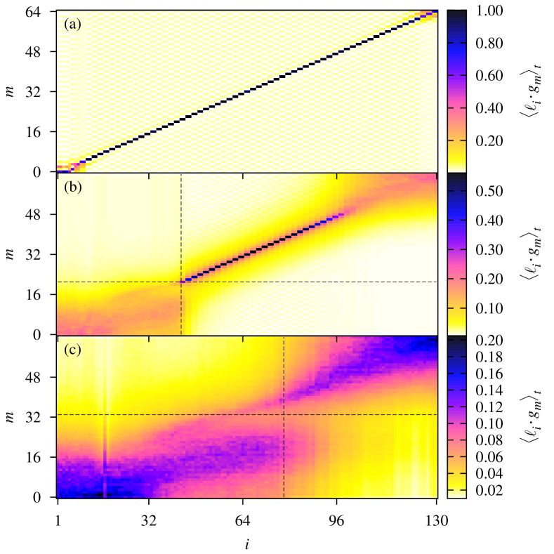
Figure 1: (color online) Average cosines of the angles between CLVs $\ell_{i}$ (horizontal axis) and eigenmodes $g_{m}$ (vertical axis). (a) $h=0.1$; (b) $h=0.5$, $i=42$ for the vertical dashed line and $m=21$ for the horizontal one; (c) $h=0.8$, $i=77$, $m=33$.

There is an area in the left bottom corner of Fig. 1(a) where CLVs differ significantly from the eigenmodes. In Ref. EffDim such kind of vectors has been called “physical”. We shall refer to them as active vectors. These vectors are discussed in the following section.

III Strict mode splitting

III.1 Angles with eigenmodes

The number of active vectors at $h=0.1$ is small because the system is close to the bifurcation point. In Fig. 1(b) $h=0.5$, and the system has 9 positive Lyapunov exponents. We observe now a large area of active vectors that is clearly separated from the set of isolated vectors. The isolated vectors are represented by the diagonal structure. The diagonal is not so sharp as in panel (a), which means that now angles between isolated vectors and corresponding eigenmodes, though small, are not equal to zero. Correspondingly, these vectors are not quite orthogonal to all other eigenmodes. But nevertheless, the isolated vectors remain very close to the eigen modes. The split between isolated and active modes is marked by the vertical dashed line at $i=42$. Also, the area of active modes is bounded from above: the horizontal dashed line is drawn at $m=21$. It means that the active vectors have relatively small angles only with “their own” eigenmodes, i.e., with eigenmodes with numbers corresponding to the active vectors. The angles with the other eigenmodes are much higher. Thus, the set of active vectors span approximately the same subspace as the corresponding amount of the eigenmodes.

There is another non-trivial structure at the right top corner of Fig. 1(b). The nature of this area is unclear yet, but we conjecture that it consists of active vectors that becomes relevant when time is reversed.

III.2 Fraction of DOS violation

The isolated modes do not have tangencies with the active modes EffDim . The method of detection of this strict mode splitting, suggested in Ref. EffDim , employs a concept of domination of Oseledec splitting (DOS) DOS1 ; DOS2 . We recall that for almost every time every vector in the tangent space $\mathcal{S}_{1}(t)$ of a dynamical system grows asymptotically at rate given by the first Lyapunov exponent $\lambda_{1}$ except those belonging to a set $\mathcal{S}_{2}(t)$ of measure zero. Similarly, almost every vector in $\mathcal{S}_{2}(t)$ asymptotically grows at rate $\lambda_{2}$ except those belonging to a set $\mathcal{S}_{3}(t)$ of measure zero relative to $\mathcal{S}_{2}(t)$, and so on. Collection of sets $\mathcal{S}_{i}(t)$ embedded one into another is called the Oseledec splitting of the tangent space. The splitting is called dominated if each Oseledec subspace is more expanded than the next, by a definite uniform factor. Let $\lambda_{i}(t,\tau)$ be the $i$-th local Lyapunov exponent, computed at time $t$ and averaged over an interval $\tau$. The Oseledec splitting is dominated at $i$ if $\lambda_{i}(t,\tau)>\lambda_{j}(t,\tau)$ holds for all $j>i$, and for all $t$ with $\tau$ larger then some finite $\tau_{0}$ EffDim . In particular, domination implies that the angles between the Oseledec subspaces are bounded from zero DOS2 .

Employing the ideas of numerical verification of DOS suggested in Refs. Psplit ; DOSV ; EffDim ; YRRev we define the fraction of DOS violation in the following manner. Fix an interval $\tau$ and compute $\lambda_{i}(t,\tau)$ for some time $t$. The violation of DOS takes place if $\lambda_{i}(t,\tau)\leq\lambda_{j}(t,\tau)$ for $j>i$. Thus, for each $i$ we check this inequality at $j>i$ and add 1 to the $i$-th site of an array if it holds at least ones. Repeating this procedure for different times and performing an averaging we obtain the fraction of DOS violation at $\tau$, which formally can be defined as $\nu_{\tau}^{(i)}=\left<\Theta\left(\max_{j>i}\left[\lambda_{j}(t,\tau)-\lambda_{i}(t,\tau)\right]\right)\right>_{t}$, where $\Theta(z)$ is the step function and $<\ldots>_{t}$ denotes the time average.

In the case of multiplicity $\lambda_{i}=\lambda_{i+1}$, corresponding $\nu_{\tau}^{(i)}$ is close to 0.5 because of fluctuations of local Lyapunov exponents due to a numerical noise. Otherwise $\nu_{\tau}^{(i)}$ decays to zero as $\tau$ grows. In general, the decay is asymptotic, but if the splitting is dominated at $i$, the corresponding fraction $\nu_{\tau}^{(i)}$ vanishes at finite $\tau_{0}$. Unfortunately, there is no a well-grounded algorithm of computation of $\tau_{0}$ except the straightforward observation of $\nu_{\tau}^{(i)}$ as a function of $\tau$. Because the law of the decay of $\nu_{\tau}^{(i)}$ is unknown a priori, there is no idea how to extrapolate of $\nu_{\tau}^{(i)}$ to zero to verify if a finite $\tau_{0}$ exists. But, anyway, in points of dominated splitting $\nu_{\tau}^{(i)}$ decays much faster against $\tau$ than elsewhere. It means that if $\tau$ is sufficiently large, a graph $\nu_{\tau}^{(i)}$ against $i$ provides relevant information about locations of the splitting.

Figure 2: (a) Fraction of DOS violation at $\tau=51.2$ vs. number of Lyapunov exponent. (b) Average projection of the state vector onto vector-columns of $Q$ vs. the number of vector. Dotted vertical lines marks, from left to right: index of the first of two zero Lyapunov exponents $i=10$, Kaplan–Yorke (Lyapunov) dimension rounded up to the next integer $i=19$, and the number of active vectors $i=42$.

Figure 2(a) shows the fraction of DOS violation at $h=0.5$. The sharp minimum of $\nu_{\tau}^{(i)}$ at $i=42$ coincides with the position of the splitting found in Fig. 1(b). This minimum, presuming the vanish of $\nu_{\tau}^{(i)}$ at a finite $\tau$, means that the active modes are hyperbolically isolated from all the rest ones. The active vectors, located to the left from the splitting point, have sufficiently high $\nu_{\tau}^{(i)}$. In this case $\nu_{\tau}^{(i)}$ vanishes only asymptotically which, in turn, indicates frequent tangencies between the active vectors. The isolated vectors are represented by a series of sharp minima and maxima with the period 2. Above we have shown that these vectors at $h=0.5$ are very close to the eigenmodes $g_{m}$. Because of the degeneracy, the modes $g_{m}$ and $g_{-m}$ have identical growth rates. Hence, there are couples of corresponding isolated vectors $\ell_{i}$ with identical growth rates. In turn, this implies the multiplicity of corresponding Lyapunov exponents. Indeed, the spectrum of Lyapunov exponents demonstrates a stepwise behavior to the right from the splitting point $i=42$ and the step is 2, see Fig. 3. (The stepwise structure of the Lyapunov spectrum corresponding to isolated vectors was also reported in Ref. EffDim .) Thus, the maxima of $\nu_{\tau}^{(i)}$ in Fig. 2(a) are associated with this multiplicity. The deep minima indicate the absence of tangencies between isolated vectors because of the orthogonality of corresponding eigenmodes.

Figure 3: Lyapunov spectrum at $h=0.5$. The horizontal dashed line mark $\lambda_{i}=0$, and the vertical ones are drawn at the same positions as in Fig. 2

The curve of $\nu_{\tau}^{(i)}$ in Fig. 2(a) demonstrates two more interesting features. We observe another point of splitting at $i=19$ where $\nu_{\tau}^{(i)}$ has a very deep minimum. The Kaplan–Yorke (Lyapunov) dimension in this case is $D_{\text{L}}\approx 18.2$. Thus, we can conjecture, that there are two types of active modes that are hyperbolically isolated from each other, and the amount of the first type modes is equal to the Kaplan–Yorke dimension rounded up to the next integer.

Also notice the sharp spike at $i=10$. To explain the emergence of this spike we need to recall that the complex Ginzburg–Landau equation with no-flux boundary conditions has two zero Lyapunov exponents SymCGLE1 ; *SymCGLE2. There are 9 positive exponents and $\lambda_{10}=\lambda_{11}=0$, so the spike at $i=10$ indicates the multiplicity of two corresponding $\ell_{i}$.

III.3 Projections of the state vectors

The split of CLVs onto active and isolated vectors should have a clear and visible manifestation in the dynamics of a system. The idea that the number of active vectors $i$ is an effective dimension of the system, suggested in EffDim , presumes that there exists a local basis where the state vector has only $i$ nonzero components. We consider projection of the state vector of the system at time $t$ on the local basis composed of backward Lyapunov vectors. These vectors are orthogonal to each other and span the same subspaces as CLVs AGuide . The backward Lyapunov vectors can be computed much faster then CLVs in the course of the standard procedure of computation of the Lyapunov exponents Benettin , because the columns of orthogonal matrices $Q$ converge to them AGuide ; ErshPotap . So, we multiply transposed matrices $Q^{\text{T}}$ by corresponding state vectors, accumulate absolute values of obtained projections, and then average them over large number of steps. (In general case, the homogeneous steady state should be subtracted from the state vector before the multiplication to avoid an unnecessary shift. But for our system the homogeneous steady state is 0.)

The average projection denoted as $s_{Q}$ is shown in Fig. 2(b). We observe the curve that agrees good with $\nu_{\tau}^{(i)}$. Projections onto active vectors are large, while they are almost zero for the isolated vectors. These two parts of the curve are clearly separated exactly at $i=42$. This clarifies the nature of the discussed mode splitting: We indeed observe that the number of active vectors can be an effective dimension of the system. Also notice that the largest component of the projection has an index which is equal to the Kaplan–Yorke dimension rounded up to the next integer, as marked by the middle dashed line in the figure.

The idea of using backward Lyapunov vectors in dimension reduction methods has already been considered and rejected as non-promising in Refs. Proj1 ; Proj2 ; Proj3 . Indeed, the validity of this basis is not so obvious. Reasoning formally, one can imagine an attractor that has inappropriate orientation in the phase space so that the decomposition fails to give correct result. But on the other hand, let us assume that we have a small spherical cloud of points that surrounds a homogeneous steady state in the phase space. When the points evolve, the cloud is extended along the most unstable manifold. In this case the most information about dynamics is positively carried by the first several CLVs. We can guess, that this property survives later producing the split into active and isolated vectors. Anyway, at least for the Ginzburg–Landau equation this decomposition gives very appropriate information concerning the mode splitting.

The picture illustrated in this section for $h=0.5$ is quite generic. We can observe the strict splitting of active and isolated modes as well as the Kaplan–Yorke mode splitting for a wide range of $h$. But when $h$ becomes sufficiently high, the situation becomes quite different, as will be discussed in the following section.

IV Fussy mode splitting

As discussed above, exactly at the bifurcation point CLVs coincide with eigenmodes and all of them are isolated, while the set of active vectors is empty. There are $2N-2$ isolated modes. When $h$ grows, the isolated modes are converted into active ones and this conversion occurs at both ends of the spectrum. (Compare small structures at the ends of the main diagonal in Fig. 1(a) and the large areas in Fig. 1(b).) At the left end the isolated modes contribute to the set of active modes, while at the right end they fill up the other set of modes, which are, conceivably, relevant when time is reversed. Figure 4 shows that the number of active modes depends on $h$ almost linearly. Because we have a finite number of modes, there is a finite $h$ for which all isolated modes are converted so that the splitting vanishes. If the conversion at both ends of the spectrum takes place symmetrically, then the isolated modes disappear when there are $N-1$ active modes. In Fig. 4 the splitting of modes indeed disappears when the number of active modes is close to 64 at $N=65$.

Figure 4: Number of active vectors against the coupling parameter $h$.

The value of $h$ where the mode splitting disappears depends on the number of eigenmodes, that, in turn depends on the number of oscillators in the chain $N$. Taking into account almost linear dependance of the number of active modes against $h$ we conclude that in a chain with an infinite number of oscillators the mode splitting vanishes at infinite $h$. Thus, the continuous system can have the mode splitting at any strength of the spatial coupling. In particular, it gives a criterion of correctness of a chain as a model of continuous system: the chain can model a continuous system only if the step size is below the point where the mode splitting vanishes.

Now we consider the tangent space above the point of mode splitting vanishing. Figure 1(c) demonstrates angles between CLVs and eigenmodes at $h=0.8$ (there are 17 positive Lyapunov exponents in this case). One can see that this figure differs much from the panels (a) and (b). Sets of vectors are still distinguishable, but their boundaries are not strict. The isolated vectors are absent at all. The vertical dashed line marks an approximate boundary between two clusters of vectors, and the horizontal one separate the spectrum of eigenmodes onto two halves. The vectors from the left cluster have relatively small angles with the first half of the spectrum of eigenmodes, while the right cluster contains the vectors that have relatively small angles with the second half of the spectrum. In particular, it means that tangencies within the clusters occur more often than between the representatives of two clusters. It can be treated as a fussy mode splitting: The left cluster is preliminary relevant to the forward time dynamics, while the right one, though also involved, but does not include much. In the reverse time the roles of the clusters are exchanged.

Figure 5: Same as Fig. 2 at $h=0.8$. The vertical dashed lines are plotted at $i=17$, $i=30$ and $i=77$.

Figure 5 shows the fraction of DOS violation and average projections of the state vector onto backward Lyapunov vectors at $h=0.8$. There is no series of sharp minima and maxima representing isolated modes, and also there is no sharp step in the curve of projections. But the curve of projections indicates that the state vector still has preferable directions inside the left cluster of CLVs, whose boundary is marked by the vertical dashed line. In the other words, the number of vectors in the left cluster can be considered as approximate effective dimension of the system. The projections to vectors from the right cluster is much smaller.

Notice also that two other features of these curves survive. We still can see the minimum of $\nu_{\tau}^{(i)}$ and the maximum of the projection corresponding to the Kaplan–Yorke dimension rounded up to the next integer, as well as the spike, indicating degeneracy associated with two zero Lyapunov exponents.

V Summary

We studied the splitting of modes of perturbations, represented by the covariant Lyapunov vectors, into sets of active and isolated modes EffDim . We considered a chain of amplitude equations obtained from the Ginzburg–Landau equation by substitution of the second spatial derivative with its finite–difference representation. The size of the step of spatial discretization was used as a control parameter while the number of oscillators in the chain was held constant. When the step size is asymptotically small, the system approaches from above the bifurcation point where the homogeneous steady state looses its stability, while increasing of the step results in more independent dynamics of oscillators.

At the bifurcation point there are no active modes. All modes are isolated and coincide with eigenmodes of the homogeneous steady state. Their spatial structure is determined by the number of oscillators and boundary conditions. When the system leaves the bifurcation point as the step size grows, the isolated modes are converted into active ones so that the number of active modes grows linearly with the step size.

For the considered system, the backward Lyapunov vectors was shown to be an appropriate basis where a number of essential components of the state vector is equal to the number of active vectors. In other words, the number of active vectors indeed plays the role of an effective dimension of the system, as conjectured in EffDim .

The active modes were found to be split into two subsets that are hyperbolically isolated from each other. The coordinate of the splitting point is equal to the Kaplan–Yorke dimension rounded up to the next integer. We conjecture that this indicates the existence of two types of active modes. The nature of these different types is unclear yet, and more studies are required.

At the right end of the spectrum we observed another set of modes which is similar to the set of active modes. Its nature is unclear yet, but we conjecture that these modes become relevant when time is reversed.

At a certain finite value of the step size the strict mode splitting disappears. Because this value depends on the number of oscillators in the chain, the vanish of the splitting occurs only for a system with finite number of degrees of freedom and probably can not be observed, in particular, for continuous systems. It can be used as an estimation of the maximum step size of the spatial discretization. If a continuous system has the strict mode splitting and its discrete model does not have it, it means that the step size is too large.

Above the point where the splitting vanishes the spectrum of modes contains two clusters without strict boundaries. This can be treated as a fussy mode splitting. The first cluster contains formerly active modes, while the other one corresponds, apparently, to the modes mainly involved when time is reversed. The projection of the state vector on the backward Lyapunov vectors indicates that the number of vectors in the first cluster could be an approximation of an effective dimension of the system.

- (1) J. C. Robinson, “Finite-dimensional behavior in dissipative partial differential equations,” Chaos 5, 330–345 (1995)
- (2) H.-L. Yang, K. A. Takeuchi, F. Ginelli, H. Chaté, and G. Radons, “Hyperbolicity and the effective dimension of spatially-extended dissipative systems,” Phys. Rev. Lett. 102, 074102 (2009)
- (3) B. Legras and R. Vautard, “A guide to lyapunov vectors,” in Predictability, ECWF Seminar, Vol. 1, edited by T. Palmer (ECMWF, Reading, UK, 1996) pp. 135–146
- (4) G. Benettin, L. Galgani, A. Giorgilli, and J. M. Strelcyn, “Lyapunov characteristic exponents for smooth dynamical systems and for hamiltonian systems: A method for computing all of them. Part I: Theory. Part II: Numerical application,” Meccanica 15, 9–30 (1980)
- (5) S. V. Ershov and A. B. Potapov, “On the concept of stationary Lyapunov basis,” Physica D 118, 167–198 (1998)
- (6) F. Ginelli, P. Poggi, A. Turchi, H. Chaté, R. Livi, and A. Politi, “Characterizing dynamics with covariant Lyapunov vectors,” Phys. Rev. Lett. 99, 130601 (2007)
- (7) C. L. Wolfe and R. M. Samelson, “An efficient method for recovering lyapunov vectors from singular vectors,” Tellus, Ser. A 59A, 355–366 (2007)
- (8) I. S. Aranson and L. Kramer, “The world of the complex Ginzburg-Landau equation,” Rev. Mod. Phys. 74, 99–143 (2002)
- (9) C. Pugh, M. Shub, and A. Strakov, “Stable ergodicity,” Bull. Am. Math. Soc. 41, 1–41 (2004)
- (10) J. Bochi and M. Viana, “The lyapunov exponents of generic volume-preserving and sympletic maps,” Ann. Math. 161, 1423–1485 (2005)
- (11) H.-L. Yang and G. Radons, “Lyapunov spectral gap and branch splitting of lyapunov modes in a diachotomic system,” Phys. Rev. Lett. 99, 165101 (2007)
- (12) H.-L. Yang and G. Radons, “When can one observe good hydrodynamic lyapunov modes?.” Phys. Rev. Lett. 100, 024101 (2008)
- (13) H.-L. Yang and G. Radons, “Lyapunov modes in extended systems,” Phil. Trans. R. Soc. A 367, 3197–3212 (2009)
- (14) P. J. Aston and C. R. Laing, “Symmetry and chaos in the complex Ginzburg-Landau equation. I. Reflectional symmetries,” Dynamics and Stability of Systems 14, 233–253 (1999)
- (15) P. J. Aston and C. R. Laing, “Symmetry and chaos in the complex Ginzburg-Landau equation. II. Translational symmetries,” Physica D 135, 79–97 (2000)
- (16) R. H. Kraichnan, “Reduced description of hydrodynamic turbulence,” J. Stat. Phys. 51, 949–963 (1988)
- (17) L. Keefe, “Properties of Ginzburg-Landau attractors associated with their Lyapunov vectors and spectra,” Phys. Lett. A 140, 317–322 (1989)
- (18) R. Grappin and J. Léorat, “Lyapunov exponents and the dimension of periodic incompressible Navier-Stokes flows: numerical measurements,” Journal of Fluid Mechanics 222, 61–94 (1991)