PHYSICS OF ELECTROWEAK INTERACTIONS WITH NUCLEI

Abstract

In this series of lectures it is illustrated how one can study the strong dynamics of nuclei by means of the electroweak probe. In particular, the most important steps to derive the cross sections in first order perturbation theory are reviewed. In the derivation the focus is put on the main ingredients entering the hadronic part (response functions), i.e. the initial and final states of the system and the operators relevant for the reaction. Emphasis is put on the electromagnetic interaction with few-nucleon systems. The Lorentz integral transform method to calculate the response functions ab initio is described. A few examples of the comparison between theoretical and experimental results are shown. The dependence of the response functions on the nuclear interaction and in particular on three-body forces is emphasized.

Emphasis is put on the electromagnetic interaction.

1 Introduction

Electroweak (e.w.) probes are essential to study the structure and the dynamics of nuclei. They help to shed light on the most fundamental nuclear physics issues. In particular they allow

• to assess the relevant degrees of freedom (d.o.f.) describing a nucleus. Traditionally these d.o.f. are supposed to be baryons and mesons. They are called “effective” d.o.f. to distinguish them from the fundamental d.o.f. of the strong interaction, i.e. quarks and gluons. Only in certain conditions of energy and momentum transferred by the e.w. probe to the nucleus they become relevant to interpret experimental results. These traditional effective d.o.f. of nuclear physics can also be divided in explicit and implicit ones. The former are those appearing in the Hamiltonian explicitly, namely the protons and the neutrons, the latter are hidden in the potential. A classical example of the latter d.o.f. is the pion implicit in the One-Pion-Exchange Potential (OPEP).

• to assess the potential model. Nowadays various realistic nucleon nucleon (NN) potentials are available, that reproduce thousands of NN scattering data with very high precision. While they are all equivalent in describing the strong NN reaction, they are not, in principle, in describing a nuclear system undergoing an e.w. reaction. Therefore, by means of an e.w. probe one hopes to be able to discriminate among them, and have a better information about their origin. Moreover, since the nuclear potential has an effective nature operating between composite systems, it is in principle a many-body operator. An aspect of nuclear dynamics that has attracted a lot of interest in the last years is the importance of multi-nucleon forces and in particular of the three-nucleon force (3NF). Electroweak reactions can shed some light on their importance and origin.

• to help understanding, by comparing theory and experiment, the microscopic origin of typical many-body phenomenologies, like for example collectivity, clusterizations or typical single particle (mean field) behaviors.

The e.w. probe is mediated by the photon $\gamma$ or by the $W^{\pm},Z_{0}$ gauge bosons. The coupling constants are small: the electromagnetic one $\alpha$ is 1/137, and the weak one is even suppressed by a factor $10^{-5}$, due to the large mass of the weak gauge bosons. Therefore in calculating e.w. cross sections with hadrons it is perfectly legitimate to use the Born approximation, i.e. the one vector-boson approximation. This has the practical consequence to allow to separate the known information about the e.w. interaction from the unknown strong one.

The plan of these notes is the following.

In the first section I will outline the main steps which bring to the derivation of the e.w. cross section with an hadron. Extensive derivations can be found in a series of both classical and more modern books and articles (see e.g.  Bjorken64 -Amaro05 ). I will deal with the electron scattering cross section as an example, suggesting how the procedure is modified in other lepton scattering cases. The photoabsorption cross section will be viewed as a particular case of the electron scattering cross section.

The second section will be an intermezzo to recall the scope of e.w. studies and to point out the interesting parts of the whole formalism.

The third section will be devoted to one of the main ingredients of the cross section i.e. the four-current operator and its connections to the potential.

In the fourth section a few considerations about the importance of ab initio approaches and of the study of few-body systems will be made, giving a short overview of the theoretical problems and how they are treated in the literature.

The fifth section will be devoted to review the Lorentz integral transform (LIT) method LIT_REPORT , describing also its practical implementation.

In the sixth section an overview of interesting applications of the LIT method to electromagnetic cross sections will be given, concentrating in particular on what can be learned about the multi-nucleon nature of the nuclear force.

Finally it will be concluded summarizing the main messages contained in these notes.

2 Outline of the derivation of electroweak cross sections

2.1 General considerations

In this section I describe how it is possible to get information on the dynamics of a nucleus (and of an hadron system in general) letting it interacts with an e.w. field and measuring the relative cross section. What I want to put in evidence in the theoretical derivation of this cross section are the matrix elements $<f_{h}|j_{h}|i_{h}>$. Here the initial and final state of the hadron are indicated by $|i_{h}>$ and $|f_{h}>$ respectively and $j_{h}$ is the four-current density operator (excitation operator) which is responsible for the internal excitation of the target, via the interaction with the external field. As was already mentioned in the introduction I specialize to the case of electron scattering, suggesting how the procedure is modified in other lepton-scattering cases. The photoabsorption cross section will be viewed as a particular case of the electron scattering cross section. Let’s repeat that we work within the one photon exchange approximation, which is depicted in figure 1. In figure 1(a) $e$ and $e^{\prime}$ represent the electron before and after the scattering, $k$ and $k^{\prime}$ are its initial and final four-momenta. Therefore one has:

$$k=(E,\vec{k})\,,\,\,\,k^{\prime}=(E^{\prime},\vec{k}^{\prime})\,,\,\,\,E^{2}-|\vec{k}|^{2}=E^{\prime 2}-|\vec{k}^{\prime}|^{2}=m_{e}^{2}\,.$$ (1)

Momentum and energy transferred by the electron to the nucleus are indicated by $\vec{q}$ and $\omega$, respectively:

$$\vec{q}=\vec{k}-\vec{k}^{\prime}\,,\,\,\,\omega=E-E^{\prime}\,,\,\,\,\omega^{2}-|\vec{q}|^{2}\equiv q^{2}\equiv-Q^{2}\,.$$ (2)

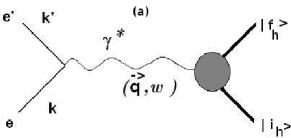
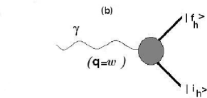
Figure 1: (a) Electron scattering in the one-photon exchange approximation, (b) photoabsorption.

In figure 1(a) $\gamma^{*}$ indicates the so called virtual photon. Its virtuality is given by the fact that $q^{2}$ (i.e. the square of the mass of this exchanged photon) is not zero, and even negative. This means that $Q^{2}$ is positive as it is demonsrarted in the following.

$$Q^{2}\,=\,{|\vec{q}|}^{2}\,-\,\omega^{2}\, = \,{\big{(}|\vec{k}|\,-\,|\vec{k}^{\prime}|\,\big{)}}^{2}\,-\,{(E\,-\,E^{\prime})}^{2}$$

$$= \,{|\vec{k}|}^{2}\,+\,{|\vec{k}^{\prime}|}^{2}\,-\,2\,\vec{k}\cdot\vec{k}^{\prime}\,-\,E^{2}\,-\,{E^{\prime}}^{2}\,+\,2\,E\,E^{\prime}$$

$$= {|\vec{k}|}^{2}\,+\,{|\vec{k}^{\prime}|}^{2}\,-\,2\,|\vec{k}|\,|\vec{k}^{\prime}|\,\cos{\theta}\,-\,{|\vec{k}|}^{2}\,-\,{|\vec{k}^{\prime}|}^{2}\,+\,2\,|\vec{k}|\,|\vec{k}^{\prime}|$$

$$= \,2\,|\vec{k}|\,|\vec{k}^{\prime}|\,(1\,-\,\cos{\theta})$$

$$= \,4\,|\vec{k}|\,|\vec{k}^{\prime}|\,{\sin^{2}{\frac{\theta}{2}}}\geq 0\,.$$

Similar pictures as in figure 1(a) can be drawn for other lepton scattering processes. One has simply to replace the electron with the lepton of interest and the photon with the appropriate gauge boson. In the limit $Q^{2}=0$ the photon becomes real. Therefore the picture describing photoabsorption becomes figure 1(b).

The advantage of studying an electron scattering process with respect to photoabsorption is the fact that one can vary energy and momentum transfer independently. Therefore one may explore the cross section in the $\omega|\vec{q}|$ plane. This aspect is strictly connected with the possibility of investigating the dynamics of the nucleus not only at different excitations but also at different ranges, being even able to realize the composite internal structure of nucleons. This happens at high momentum transfer when the wavelength associated to $|\vec{q}|$ is comparable or smaller than the nucleon size. The only restriction is the so called space-like condition $Q^{2}\geq 0$. Furthermore, in contrast to hadron probes, the virtual photon, as the real one, has a much larger mean free path, so that it can explore the whole target volume. In fact hadron probes tend to interact only on the surface.
The large flexibility of the electrons with respect to hadrons and real photons reflects on the structure of the cross section. As we will see this contains longitudinal and transverse components, which allow one to have different detailed informations about nuclear dynamics.

Our starting point is the differential cross section defined as follows:

$$d\sigma\,=\,{\frac{|{\mathcal{M}}_{if}|^{2}}{VT|\vec{j}_{i}^{e}|\rho_{target}}}\,\,{d\vec{k}^{\prime}}\,{d\vec{P}_{f}}\,\rho_{f}\,,$$ (3)

where $|{\mathcal{M}}_{if}|^{2}$ is the probability that the system goes from the initial to the final state (lowest order S-matrix) i.e. $|{\mathcal{M}}_{if}|^{2}=\frac{1}{2}\sum_{s,s^{\prime}}|<F|H_{int}|I>|^{2}$ with $|I>$ and $|F>$ the initial and final states of the whole system (incident electron $+$ target); $|\vec{j}_{i}^{e}|$ is the incident electron flux and the sum and average over the spin states of the initial and scattered electron $s$ and $s^{\prime}$ mean that we restrict to unpolarized electrons. The phase space density $\rho_{f}$ is connected to the differential momenta of the fragments:

• if the hadron remains intact   $\rho_{f}=1$

• if the hadron breaks into 2 fragments $\,\Rightarrow\,d\vec{P}_{1}\,d\vec{P}_{2}\,=\,d\vec{P}_{f}\,d\vec{p}$ i.e.  $\rho_{f}$  =  $d\vec{p}$

• if the hadron breaks into 3 fragments $\,\,\Rightarrow\,\,d\vec{P}_{1}\,d\vec{P}_{2}\,d\vec{P}_{3}\,=\,d\vec{P}_{f}\,d\vec{p}_{1}\,d\vec{p}_{2}$  etc., where $\vec{P}_{f}$ is the final momentum of the hadron center of mass (c.m.), while the $\vec{p}_{i}$ indicate the relative momenta of the fragments.

In the next subsection we will elaborate on the matrix element $<F|H_{int}|I>$, however, as already mentioned, what is important for us is the part which regards the target $<f_{h}|j_{h}|i_{h}>$, because the internal dynamics of the system is contained in that. Therefore in following the evolution of the formulas one has to keep the focus on that matrix element.

It is interesting to note that one can perform several different kinds of experiments with the electromagnetic probe. One can make elastic scattering experiments where the nucleus is not excited and the energy transferred by the lepton is found exclusively in the target recoiling energy (of course this is never the case for photons). When this happens one has $|i_{h}>=|f_{h}>$. Therefore in such experiments the focus is on bound state properties of the nucleus. If the energy transfer serves in addition to excite the nucleus one speaks of inelastic scattering. In this case the information contained in the cross section is not only on the bound state, but also on the excited states. Depending on the energy transfer (and of the nucleus) they can be discrete states or continuum (break-up) states. One can also study absorption or emission of photons.

If the energies and momenta do not exceed a few hundred of MeV, and the nuclei contain a not too large number of protons a good theoretical framework for calculating the cross sections of all these processes consists of first order (one-photon-exchange approximation) quantum electro-dynamics (QED) and non relativistic quantum mechanics. For heavier nuclei the first order can become questionable. Since in the following I will concentrate mainly on light nuclei this problem has no relevance.

2.2 The transition matrix

Let us now discuss the ingredients of the transition matrix ${\mathcal{M}}_{if}=<F|H_{int}|I>$ whose square modulus is the main term in the cross section.

The interaction Hamiltonian is

$$H_{int}=\int d^{4}xj^{e}_{\mu}(x)\cdot A^{\mu}(x)\,,$$ (4)

where $j^{e}_{\mu}(x)$ is the four-current density of the electron and $A^{\mu}(x)$ is the electromagnetic four-potential created by the target,

$$A^{\mu}(x)=\int d^{4}yD_{F}(x-y)j_{h}^{\mu}(y)\,,$$ (5)

where $D_{F}(x-y)$ is the Feynmann propagator.

The incident electron current is

$$j^{e}_{\mu}=-e\bar{\psi}(x)\gamma_{\mu}\psi(x)\,,$$ (6)

where $\psi(x)$ is the Dirac spinor $\sqrt{\frac{m}{EV}}u(k,s)e^{-ik\cdot x}$. Therefore one has:

$$<F|H_{int}|I> = {-\int d^{4}\,x\,\,em\over\sqrt{EE^{\prime}}V}\bar{u}(k^{\prime},s^{\prime})\,\gamma_{\mu}\,u(k,s)<e^{ik^{\prime}\cdot x}|\int d^{4}\,y\,D_{F}(x-y)|e^{-ik\cdot x}>\cdot$$ (7)

$$\cdot <f_{h}|e^{iP_{f}\cdot y}\,j_{h}^{\mu}\,e^{-iP_{i}\cdot y}|i_{h}>{1\over{(2\pi)^{4}}}\,.$$ (8)

Performing the integrals in $d^{4}\,y$ and $d^{4}\,x$ one gets

$$<F|H_{int}|I>={-e^{2}m\over\sqrt{EE^{\prime}}V}\bar{u}(k^{\prime},s^{\prime})\gamma_{\mu}u(k,s)\int{d^{4}q\over q^{2}}\delta^{(4)}(k^{\prime}-k+q)\delta^{(4)}(P_{f}-P_{i}-q)J^{\mu}\,.$$ (9)

Notice: It is here that the matrix element of interest $<f_{h}|j^{\mu}_{h}|i_{h}>$ appears. For economy of notations it has been denoted simply by $J^{\mu}$.

The integral in $d^{4}\,q$ gives

$$<F|H_{int}|I>={-e^{2}m\over\sqrt{EE^{\prime}}V}\bar{u}(k^{\prime},s^{\prime})\gamma_{\mu}u(k,s){\delta^{(4)}(P_{f}-P_{i}+k^{\prime}-k)\over q^{2}}J^{\mu}\,,$$ (10)

where $q=k-k^{\prime}=P_{f}-P_{i}$.

The lepton and hadron tensors

If one inserts this expression in the transition probability and use the following relation Bjorken64

$$[{(2\pi)}^{4}\,\delta^{(4)}\,(P_{f}-P_{i}\,+\,k^{\prime}-k)]^{2}\,=\,\delta^{(4)}\,(P_{f}-P_{i}\,+\,k^{\prime}-k)\cdot V\cdot T\,{(2\pi)}^{4}\,,$$ (11)

one obtains

$$|{\mathcal{M}}_{if}|^{2}={e^{2}m^{2}\over EE^{\prime}V^{2}}{\delta^{(4)}(P_{f}-P_{i}+k^{\prime}-k)\over q^{4}}\cdot V\cdot T\sum_{s^{\prime}}|\bar{u}(k^{\prime},s^{\prime})\gamma_{\mu}u(k,s)|^{2}J^{\mu\star}J^{\nu}\,.$$ (12)

Defining the lepton tensor

$$w_{\mu\nu}\equiv|\bar{u}(k^{\prime},s^{\prime})\gamma_{\mu}u(k,s)|^{2}$$ (13)

and the hadron tensor $W^{\mu\nu}\equiv J^{\mu\star}J^{\nu}$, and considering that the electron flux can be written as $|\vec{J}_{e}|=\rho v_{i}={1\over V}{E\over|\vec{k}|}$ the differential cross section becomes

$$d\sigma={e^{4}m^{2}\over E^{\prime}|\vec{k}|}{1\over q^{4}}\sum_{s^{\prime}}w_{\mu\nu}W^{\mu\nu}\delta^{(4)}\,d\vec{k}^{\prime}\,d\vec{P}_{f}\,.$$ (14)

Manipulating the lepton tensor by using the properties of the traces of Dirac matrices one has

$$w_{\mu\nu}={2\over m^{2}}[k_{\mu}k_{\nu}^{\prime}+k^{\prime}_{\mu}k_{\nu}-g_{\mu\nu}(k\cdot k^{\prime}-m^{2})]+ih\epsilon_{\mu\nu\alpha\beta}k^{\alpha}k^{\prime\beta}]\,,$$ (15)

where $h$ is the helicity of the longitudinally polarized electron. For unpolarized electrons such a contribution vanishes. Let’s concentrate just on the part of the cross section which does not depend on the electron polarization, i.e.

$$d\sigma={e^{4}m^{2}\over E^{\prime}|\vec{k}|}{1\over q^{4}}{2\over m^{2}}[k_{\mu}k_{\nu}^{\prime}+k^{\prime}_{\mu}k_{\nu}-g_{\mu\nu}(k\cdot k^{\prime}-m^{2})]J^{\mu\star}J^{\nu}\delta^{(4)}\,d\vec{k}^{\prime}\,\,d\vec{P}_{f}\,.$$ (16)

2.3 The use of charge conservation

At this point one can make use of the continuity equation $q_{\mu}J^{\mu}=0$ (charge conservation) both for the electron and hadron currents. Remember that $d\sigma$ contains essentially ${|j^{e}_{\mu}J^{\mu}|}^{2}$. The continuity equations imply $j^{e}_{0}={{\vec{j}^{e}\cdot\vec{q}}\over q_{0}}$ and $J_{0}={{\vec{J}\cdot\vec{q}}\over q_{0}}$. Therefore

$$j^{e}_{\mu}J^{\mu}=j^{e}_{0}J^{0}-\vec{j}_{e}\cdot\vec{J}={{(\vec{q}\cdot\vec{j}_{e})(\vec{q}\cdot J)}\over{q^{2}_{0}}}-\vec{j}_{e}\cdot\vec{J}=\vec{j}_{e}\cdot\Bigg{(}\vec{q}{{(\vec{q}\cdot\vec{J})}\over{q^{2}_{0}}}-\vec{J}\Bigg{)}=\vec{j}_{e}\cdot\vec{J}^{\prime}\,,$$ (17)

with $\vec{J}^{\prime}\,=\,\vec{J}\,-\,\vec{q}{{(\vec{q}\cdot\vec{J})}\over q_{0}^{2}}$. This means that the use of the continuity equation allows to replace the 4-indexes $\mu,\nu=0,1,2,3$ with the 3-indexes $i,j=1,2,3$ and the differential cross section becomes

$$d\sigma={e^{4}\over{E^{\prime}|\vec{k}|}}{2\over q^{4}}\,\left[k_{i}k^{\prime}_{j}\,+\,k^{\prime}_{i}k_{j}\,-\,g_{ij}\,(k\cdot k^{\prime}-m^{2})\right]\,J^{\prime i*}\,J^{\prime j}\,\delta^{(4)}\,d\vec{k}^{\prime}\,\,d\vec{P}_{f}\,.$$ (18)

Using the relation   $Q^{2}\,=\,-q^{2}\,=\,-\,(2m^{2}-2k\cdot k^{\prime})$  and performing the sum on $i,j$ one gets

$$d\sigma={e^{4}\over E^{\prime}|\vec{k}|}{2\over q^{4}}\left[2Re(\vec{k}\cdot\vec{J}^{\prime*}\,\vec{k}^{\prime}\cdot\vec{J}^{\prime})+{Q^{2}\over 2}\vec{J}^{\prime*}\vec{J}\right]\delta^{(4)}\,d\vec{k}^{\prime}\,\,d\vec{P}_{f}\,.$$ (19)

2.4 Longitudinal and transverse response functions

At this point it is convenient to choose a particular Cartesian system where

$$\hat{z}=\hat{q};\,\,\,\,\hat{y}={\vec{k}\times\vec{k}^{\prime}\over|\vec{k}\times\vec{k}^{\prime}|};\,\,\,\,\hat{x}=\vec{y}\times\vec{z}$$ (20)

and decompose $\vec{J}^{\prime}$ in

$$\vec{J}^{\prime}=\vec{J}^{\prime}_{L}+\vec{J}^{\prime}_{T}\,,$$ (21)

with

$$\vec{J}^{\prime}_{L} = \hat{q}J^{\prime}_{L}=(\vec{J}^{\prime}\cdot\hat{q})\,\hat{q}$$ (22)

$$\vec{J}^{\prime}_{T} = (\vec{J}^{\prime}\cdot\hat{x})\,\hat{x}+(\vec{J}^{\prime}\cdot\hat{y})\,\hat{y}\,.$$ (23)

Using the definition of $\vec{J}^{\prime}$ and the continuity equation $J_{0}q_{0}=\vec{q}\cdot\vec{J}$ one has

$$J^{\prime}_{L}=-{Q^{2}\over\omega|\vec{q}|}\,\rho\,.$$ (24)

Substituting in (19) the target dynamics according to the decomposition (21) one obtains three different contributions to the cross section i.e. the longitudinal, transverse and mixed ones. Making use of a few kinematic relations one has

$$(d\sigma)_{L}={e^{4}\over E^{\prime}|\vec{k}|}{1\over q^{4}}{Q^{4}\over|\vec{q}^{4}|}(4EE^{\prime}-Q^{2})\,|\rho|^{2}\delta^{(4)}\,d\vec{k}^{\prime}\,\,d\vec{P}_{f}\,.$$ (25)

Analogously the transverse and mixed contributions are given by

$$(d\sigma)_{T} = {e^{4}\over E^{\prime}|\vec{k}|}{1\over q^{4}}4|\vec{k}|\,|\vec{k}^{\prime}|\left[\left({|\vec{k}|\,|\vec{k}^{\prime}|sin^{2}\theta\over 2|\vec{q}|^{2}}+{Q^{2}\over 4|\vec{k}|\,|\vec{k}^{\prime}|}\right)\left(|J^{\prime}_{x}|^{2}+|J^{\prime}_{y}|^{2}\right)\right.+$$ (26)

$$+ \left.{|\vec{k}|\,|\vec{k}^{\prime}|sin^{2}\theta\over 2|\vec{q}|^{2}}\left(|J^{\prime}_{x}|^{2}-|J^{\prime}_{y}|^{2}\right)\right]\delta^{(4)}\,d\vec{k}^{\prime}\,\,d\vec{P}_{f}\,;$$ (27)

$$(d\sigma)_{LT}={-e^{4}\over E^{\prime}|\vec{k}|}{4\over q^{4}}{Q^{2}\over|\vec{q}|^{3}}|\vec{k}|\,|\vec{k}^{\prime}|sin\,\theta\,(E+E^{\prime})Re(\rho^{\star}j^{\prime}_{x})\delta^{(4)}\,d\vec{k}^{\prime}\,\,d\vec{P}_{f}\,.$$ (28)

The transverse contribution consists of two separated terms which are indicated with the labels $T$ and $TT$ respectively. So at the end one can summarize the cross section as

$$(d\sigma)=\left(V_{L}R_{L}+V_{T}R_{T}+V_{TT}R_{TT}+V_{LT}R_{LT}\right)\delta^{(4)}\,d\vec{k}^{\prime}\,\,d\vec{P}_{f}\,,$$ (29)

where the V’s indicate the coefficients of kinematic nature and the $R$’s the structure functions containing the matrix elements characterizing the target dynamics:

$$V_{L}={e^{4}\over E^{\prime}|\vec{k}|}{1\over q^{4}}{Q^{4}\over|\vec{q}^{4}|}(4EE^{\prime}-Q^{2})\,;$$ (30)

$$V_{T}={e^{4}\over E^{\prime}|\vec{k}|}{1\over q^{4}}\,2|\vec{k}|\,|\vec{k}^{\prime}|\left({|\vec{k}|\,|\vec{k}^{\prime}|\sin^{2}\theta\over|\vec{q}|^{2}}+{Q^{2}\over 2|\vec{k}|\,|\vec{k}^{\prime}|}\right)\,;$$ (31)

$$V_{TT}={e^{4}\over E^{\prime}|\vec{k}|}{1\over q^{4}}{2|\vec{k}|\,|\vec{k}^{\prime}|\sin^{2}\theta\over 2|\vec{q}|^{2}}\,;$$ (32)

$$V_{LT}={-e^{4}\over E^{\prime}|\vec{k}|}{4\over q^{4}}{Q^{2}\over|\vec{q}|^{3}}|\vec{k}|\,|\vec{k}^{\prime}|(E+E^{\prime})\,\sin\,\theta\,;$$ (33)

$$R_{L}=|\rho|^{2}\,;$$ (34)

$$R_{T}=|J^{\prime}_{x}|+|J^{\prime}_{x}|\,;$$ (35)

$$R_{TT}=|J^{\prime}_{x}|-|J^{\prime}_{x}|\,;$$ (36)

$$R_{LT}=Re(\rho^{\star}J^{\prime}_{x})\,.$$ (37)

Equation (29) is very general. The kinematic coefficients (30)-(33) can be expressed in the non-relativistic or ultra-relativistic limits for the electron kinematics. In the ultra-relativistic limit i.e. when the mass of the electron is much smaller that its momentum (that is certainly the case for electrons of tens or hundreds of MeV) $E=|\vec{k}|$ and $E^{\prime}=|\vec{k}^{\prime}|$, then one has

$${|\vec{k}^{\prime}|}^{2}V_{L}\,=\,\sigma_{M}{{Q^{4}}\over{|\vec{q}|}^{4}}\,,$$ (38)

where

$$\sigma_{M}\,=\,{1\over{4\,E^{2}}}\,{{{\cos^{2}{\theta\over 2}}}\over{\sin^{4}{\theta\over 2}}}\,\equiv\,\sigma_{Ruth.}\,{{\cos^{2}{\theta\over 2}}}\,;$$ (39)

$${|\vec{k}^{\prime}|}^{2}V_{T}\,=\,{e^{4}\over E^{\prime}|\vec{k}|}\,{1\over q^{4}}\,2|\vec{k}|\,|\vec{k}^{\prime}|\,\left({|\vec{k}|\,|\vec{k}^{\prime}|\sin^{2}\theta\over|\vec{q}|^{2}}\,+\,{Q^{2}\over 2|\vec{k}|\,|\vec{k}^{\prime}|}\,\right)\,;$$ (40)

$${|\vec{k}^{\prime}|}^{2}V_{TT}\,=\,{e^{4}\over E^{\prime}|\vec{k}|}{1\over q^{4}}{2|\vec{k}|\,|\vec{k}^{\prime}|\sin^{2}\theta\over 2|\vec{q}|^{2}}\,;$$ (41)

$${|\vec{k}^{\prime}|}^{2}V_{LT}\,=\,{-e^{4}\over E^{\prime}|\vec{k}|}{4\over q^{4}}{Q^{2}\over|\vec{q}|^{3}}|\vec{k}|\,|\vec{k}^{\prime}|\sin\,\theta\,(E+E^{\prime})\,.$$ (42)

2.5 The cross section for inclusive, unpolarized electron scattering

From (29) one can obtain inclusive, seminclusive, exclusive, etc. cross sections according to what one is going to measure.
For example: if one wants the inclusive cross section i.e. one reveals the outcoming electron and nothing else

$${d\sigma\over d\vec{k}^{\prime}}=\int d\vec{P}_{f}\,(\,V_{L}R_{L}\,+\,V_{T}R_{T}\,+\,V_{TT}R_{TT}+V_{LT}R_{LT}\,)\,\delta^{(4)}\,(\,P_{f}\,-\,P_{i}\,+\,k^{\prime}-k\,)\,.$$ (43)

If one wants the seminclusive cross section i.e. one reveals the outcoming electron and a proton in coincidence  $(\,\rho_{f}\,=\,d\vec{p}_{P}\,)$

$${d\sigma\over{d\vec{k}^{\prime}d\vec{P}_{P}}}=\int d\vec{P}_{f}\,(\,V_{L}R_{L}\,+\,V_{T}R_{T}\,+\,V_{TT}R_{TT}\,+\,V_{LT}R_{LT}\,)\,\delta^{(4)}\,(\,P_{f}\,-\,P_{i}\,+\,k^{\prime}\,-\,k\,)\,{d\vec{p}_{P}\over{d\vec{P}_{p}}}\,,$$ (44)

where $\vec{p}_{P}$ is the momentum of the proton in the c.m. system, while $\vec{P}_{P}$ is measured in the lab. system, etc. Let us concentrate on the simplest cross section i.e. the inclusive one. This is certainly the simplest from an experimental point of view, since one only needs (besides accelerator and target) only an electron spectrometer counting the electrons with a given energy, momentum at a certain scattering angle. A seminclusive cross section requires an additional hadron spectrometer and the number of counts in coincidence will be certainly smaller (smaller cross section). From the theoretical point of view, at a first sight, the inclusive cross section does not appear to be the simplest, but on the contrary in some cases the most complicate. I will comment about this in the section where the LIT method is described.

A simplification of the expression for the cross section arises if one considers unpolarized targets. In fact in this case one has to sum and average on the target spin projections in the final and initial state, respectively. One can show that this implies that the terms $V_{TT}R_{TT}$ and $V_{LT}R_{LT}$ vanish. Therefore one has

$${d\sigma\over d\vec{k}^{\prime}}\, = \,{d\sigma\over{d\Omega_{e}\,d|\vec{k}|^{\prime}}}$$

$$= \,{k^{\prime 2}\int d\vec{P}_{f}\,(\,V_{L}R_{L}\,+\,V_{T}R_{T}\,)\,\delta^{(3)}\,(\,\vec{P}_{f}\,-\,\vec{P}_{i}\,-\,\vec{q}\,)\,\delta\,(\,E^{h}_{f}\,-\,E^{h}_{i}\,-\,\omega\,)}\,,$$

where $E^{h}_{f}\,,\,E^{h}_{i}$ represent the energies of the nucleus in the initial and final state. One has to stress here that these energies are not only the internal energies, but include the recoil energy. At this point one substitutes the matrix elements of interest in $R_{L}$ and $R_{T}$ in (34)-(35) and performs the integral in $d\vec{P}_{f}$, obtaining

$${d{\sigma}\over{d\Omega_{e}\,d\omega}}\, = \,\sigma_{M}\,\left[{Q^{4}\over{|\vec{q}|}^{4}}\,\sum_{n}\,{|\,\langle f_{n}\,|\,\widehat{\rho}\,|\,i_{h}\,\rangle|}^{2}\,\delta\,(E_{f}^{h}\,-\,E_{i}^{h}\,-\,\omega)\right.$$ (46)

$$+ \left.\left({Q^{2}\over{2{|\vec{q}|}^{2}}}\,+\,{tg}^{2}{\theta\over 2}\right)\,\sum_{n}\,{|\,\langle f_{n}\,|\,{\hat{\vec{J}}}_{T}\,|\,i_{h}\,\rangle|}^{2}\,\delta\,(E_{f}^{h}\,-\,E_{i}^{h}\,-\,\omega)\right]\,,$$

where the $\delta$-function $\delta\,(E_{f}^{h}\,-\,E_{i}^{h}\,-\,\omega)=\delta\,({\mathcal{E}}_{f}+E_{rec}-{\mathcal{E}}_{i}-\,\omega)$ with ${\mathcal{E}}_{f}$ and ${\mathcal{E}}_{i}$ indicating the internal energies and $E_{rec}$ the recoil energy acquired by the nucleus (non relativistically $E_{rec}=|\vec{q}|^{2}/2M_{A}^{2}$ with $M_{A}$ representing the mass of the nucleus).

Notice: The integral in $d\vec{P}_{f}$ has an important consequence: the operators $\widehat{\rho}$ and ${\hat{\vec{J}}}_{T}$ are function of $|\vec{q}|$ and are expressed in the c.m. system of the nucleus.

The following remarks are in order here.

• In order to get separate experimental information on $R_{L}$ and $R_{T}$ one needs to perform the so called Rosenbluth separation which consists essentially in performing two (or more) measurements of the cross section at fixed $\omega$ and $|\vec{q}|$ and different scattering angles. Representing these data in a XY plot where X = $V_{T}$ and Y is the cross section, one obtains a straight line whose properties are connected to $R_{L}$ and $R_{T}$.

• One can generalize the derivation of the cross section obtained above to take into account also the parity violating contributions. This corresponds to add to the graph in figure 1(a) a similar one with the $Z_{0}$ boson replacing the virtual photon.

• One can also generalize the procedure explained above to neutrino reactions ($\nu,\nu^{\prime}$) ($\nu,\mu^{\pm}$). In the former case the virtual photon is replaced by $Z_{0}$. In the latter case by $W^{\pm}$. Of course in these cases the coupling constant $\alpha^{2}=e^{2}/\hbar c$ is replaced by the weak one.

One can read more extensive derivations of the e.w. cross sections in Donnelly85 ; Arenhoevel01 ; Amaro05 .

3 Intermezzo

At this point, it is better to remind what is the scope of our study. In general one could distinguish two different attitudes in studying e.w. interactions with nuclei. One is what I will call the “service” attitude. It means that nuclear theorists calculate e.w. cross sections that are important to solve problems of astrophysical relevance. For example in figures 2 and 3 one can see two famous nucleosynthesis cycles for the production of ⁴He. One can notice how many e.w. reactions are involved in the cycles. To know the different reaction cross sections is important to explain the abundances of elements in the Universe. Other e.w. cross sections are fundamental to explain the stellar evolution. Many of these cross sections cannot be measured in the laboratory since it is often not possible to reproduce the astrophysical conditions. Therefore nuclear theorists try to help to estimate those cross sections, as well as they can, using, in most cases, their experience with models or experimental inputs from other sources or, in rarer cases, accurate ab initio calculations.

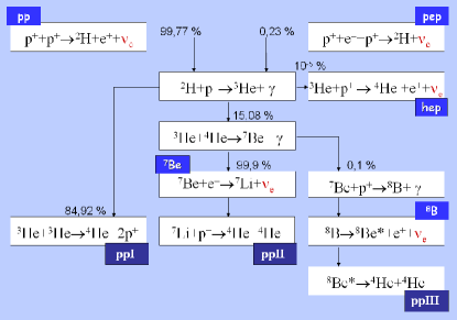
Figure 2: The proton-proton cycles for the synthesis of ⁴He

Figure 3: The Carbon-Nitrogen-Oxygen cycle for the synthesis of ⁴He

The other attitude, that I would describe as a more “fundamental” attitude consists in trying to understand what are the fundamental degrees of freedom (implicit and explicit) at the nuclear scale; what are the properties of the nuclear force and try to connect them to the underlying fundamental d.o.f. of QCD; what is the role of symmetries and their microscopic origin; what is the microscopic origin of nuclear phenomena. All that requires ab initio approaches. It means that one has to solve the many-body problem as accurately as possible, controlling the errors. Only in this case the comparison of a theoretical result, obtained with a certain input, and the experimental data gives information about how good the input is, without the uncertainties due to approximations in the solution of the many-body problem.

In deriving the inclusive unpolarized electron scattering cross section we have seen how the interesting and fundamental nuclear physics ingredients enter the cross section. They are contained in $|i_{h}\,\rangle$ and $\langle f_{h}\,|$ which are eigenfunctions of the nuclear Hamiltonian. Therefore they will be different for different nuclear potentials. However, there is more information in the cross section: in fact the nuclear charge and nuclear current operators appear. This constitutes an important difference between e.w. and purely hadron reactions. In the latter no information about charge and currents is present. This is relevant, since it gives access to what one calls underlying or implicit degrees of freedom. Let us explain this further in the next section.

4 The nuclear four-current operator

If one thinks that the most reasonable effective d.o.f. in a nuclear Hamiltonian are protons and neutrons it becomes natural to describe the interaction of the electron with the nucleus as a sum of the contributions of all the interactions with the nucleons, thought as Dirac particles with anomalous magnetic moments. However, since one then calculates the matrix elements within non relativistic quantum mechanics one has to perform a non relativistic reduction of this interaction. This can be done via the so called Foldy-Wouthousen transformation FW50 ; EISGREI88 . Essentially what one gets from such a transformation is an expression for the charge and the current operators at lowest relativistic order. The result is very intuitive. For the density operator one obtains

$$\hat{\rho}(\vec{q})=e\sum_{i=1}^{Z}\exp{(i\vec{q}\cdot\vec{r}_{i})}\,.$$ (47)

This corresponds to the Fourier transform of the sum of Z $\delta$-functions centered in the positions of the protons (as was already noticed above the positions have to be taken in the c.m. of the nucleus). In this expression $e$ is the proton charge. The neutron has no charge so it does not appear. Of course this ansatz is too drastic in that one knows that protons and neutrons have form factors. So what is done in practice is to replace $e$ with the proton form factor $G_{E}^{p}$ and sometimes even add the terms with the neutron contributions via $G_{E}^{n}$, even if in most cases they give negligible contributions.

At lowest order the expression for the transverse current is also intuitive. One gets two different currents, one due to the motion of protons, called convection current and the other due to the anomalous magnetic moments $\mu_{i}$ of both protons and neutrons, called spin current;

$$\hat{\vec{J}}_{c}=e\sum_{i}^{Z}\left\{\frac{\vec{p}_{i}}{2m},\exp{(i\vec{q}\cdot\vec{r}_{i})}\right\}\,,$$ (48)

$$\hat{\vec{J}}_{s}=\sum_{i}^{A}\mu_{i}\frac{\sigma_{i}\,\times\,\vec{q}}{2m}\exp{(i\vec{q}\cdot\vec{r}_{i})}\,.$$ (49)

However, this is not all. In fact one has to notice that $\hat{\rho},\hat{\vec{J}}$ and the Hamiltonian $\hat{H}$ are not independent. They have in fact to satisfy the continuity equation expressed by

$$\vec{\nabla}\cdot\hat{\vec{J}}=-i[\hat{H},\hat{\rho}]\,.$$ (50)

So $\hat{H}$ and ${\hat{\rho}}$ fix the divergence of the current, but not the curl, therefore they do not fix $\hat{\vec{J}}$. The convection and spin currents in (48) and (49) are one body operators. It is easy to prove that only the commutator $[\hat{T},\hat{\rho}]$ actually reproduces the divergence of $\hat{\vec{J}}$, namely one has

$$\vec{\nabla}\cdot(\hat{\vec{J}}_{c}+\hat{\vec{J}}_{s})=-i[\hat{T},\hat{\rho}]\,.$$ (51)

But then there must exist another current which is a two-(or many-)body operator which satisfies

$$\vec{\nabla}\cdot\hat{\vec{J}}^{\,exc}=-i[\hat{V},\hat{\rho}]\,.$$ (52)

Therefore one has that a given potential can only fix the divergence of this current. But what about the curl?

If the potential is based on meson theory, one of course knows the entire current. This is the current of the exchanged meson. Since this meson does not appear as an explicit degrees of freedom in the Hamiltonian, it is an implicit d.o.f.. In this sense one says that the e.w. interaction gets information on implicit degrees of freedom, namely those intermediate ones, connecting nuclear physics to the fundamental theory of strong interaction, i.e. QCD in the non perturbative regime.

Contrary to potentials based on meson theories, phenomenological potentials are not built knowing the underlying degrees of freedom. Therefore such potentials may be very accurate in reproducing nucleon-nucleon scattering data, but their reliability in electromagnetic interaction is in principle unknown since the exchange currents are not known. As already said charge conservation can give the constraint on the divergence of the currents, but no constraint on the curl exists. Therefore in order to calculate an electromagnetic cross section one must have a “model” for the underlying degrees of freedom in the potential and the comparison with electromagnetic data will allow to judge its reliability.

5 ab initio approaches and few-body physics

As already explained above ab initio calculations are those requiring the Hamiltonian $\hat{H}$, the four-current ($\hat{\rho},\hat{\vec{J}}$) (provided the consistency in (50)) and the kinematic conditions of the reaction as only inputs, treating all degrees of freedom of the many–body system explicitly and accurately (microscopic approach). Only in this way the comparison theory-experiment can be meaningful regarding the reliability of the inputs. However, ab initio approaches are a real challenge. At present only when the number of particles is relatively small one is able to get accurate solutions of the quantum mechanical many-body problem, without the need of approximations. They are necessary and unavoidable for more complex systems. From here comes the importance of few-body physics.

Solving the quantum mechanical many-body problem has very different degrees of difficulty, depending if one deals with bound or continuum states. In general the situation is particularly problematic in nuclear physics, due to the complicated structure of the nuclear potential (a brief discussion about the nuclear potential will be found later). In the following the problems of bound and continuum states are discussed separately.

5.1 Bound states

Nowadays three- and four-nucleon bound states and binding energies can be calculated with different methods based on any of the most modern high-precision NN-forces with an accuracy on the percentage level or less. For A=3 and 4 a well founded formulation, the Faddeev-Yakubovsky scheme (FY) Yakubovsky ; kamada ; Gloeckletext , opened that avenue followed by alternative, equally accurate procedures: expansions in hyperspherical harmonics (HH) A89 ; F83 ; VKR95 or gaussians (CRCGV) Kamimura88 ; Kameyama89 , stochastic variational method (SVM) c1 , and path integral techniques in form of the “Green’s Function Monte Carlo” method (GFMC) Carlson ; AV18+ ; aequal8 . Other very promising methods, based on the theory of effective interactions LS80 , have been developed: the “no-core shell model” (NCSM) Navratil99 ; Navratil00 ; Navratil00a and the “effective interaction HH” (EIHH) Barnea00 ; Barnea01 using expansions in harmonic oscillator and HH basis functions, respectively.

Table 1: Kinetic $\langle T\rangle$, potential $\langle V\rangle$, binding energy $E_{b}$ (all in MeV), and mean square radius of ⁴He as obtained by various methods. From benchmark4

. Method $\langle T\rangle$ $\langle V\rangle$ $E_{b}$ $\langle r^{2}\rangle^{1/2}$ FY 102.39 -128.33 -25.94(5) 1.485 CRCGV 102.25 -128.13 -25.89 SVM 102.35 -128.27 -25.92 1.486 HH 102.44 -128.34 -25.90(1) 1.483 GFMC 102.3(10) -128.25(10) -25.93(2) 1.490(5) NCSM 103.35 -129.45 -25.80(20) EIHH 100.8(9) -126.7(9) -25.944(10) 1.486

An example of the degree of accuracy reached by these methods in the four-body system is given in table 1 benchmark4 , where binding energy, expectation values of kinetic and potential energies and mean square radius of ⁴He are shown as they result from calculations of seven different techniques based on the same potential model. By the way, remembering that the experimental value of ⁴He is 28.3 MeV one can say that the most precise techniques lead to a clear cut answer: the potential used in benchmark4 underbinds the $\alpha$-particle significantly. This is no accident. It turns out that all modern realistic NN-forces underbind light nuclei significantly, showing the importance of three-body force (see below).

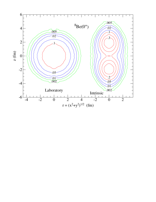
Figure 4: Upper panel: calculated spectra of A=6-8 nuclei from wiringa00 ; lower panel: calculated density contours of the ⁸Be ground state in the lab frame(left) and the intrinsic frame (right), labeled with densities in fm^-3.

While very light nuclei ($A=2-4$) are privileged systems for the study of fundamental issues like properties and origin of the strong force, as is for example the existence of the multi-nucleon forces, the ab initio study of bound state properties of heavier nuclei has its own merit with respect to new many-body phenomena like, e.g., clusterization. Furthermore, one can expect that in heavier systems some of the interaction phenomena found in light nuclei may be modified or amplified in view of the higher average nucleon density (“medium effects”).

Going beyond four-body nuclei, the low-lying spectra for up to A=8 nucleons is rather well described wiringa04 , as shown in table 2. Also these results clearly show that, in relation to the most modern NN-forces, 3N-forces are unavoidable in order to describe binding energies and low-lying excited states of light nuclei. Since the number of nucleon triplets overtakes more and more the number of nucleon pairs with increasing A, it is clear that 3N-forces have to be included as well in any realistic description of complex nuclei.

Table 2: Experimental and GFMC energies (in MeV) of particle-stable or narrow-width nuclear states. Monte Carlo statistical errors in the last digits are shown in parentheses. AV18 indicates the phenomenological NN potential AV18 , while IL stands for a version of the Urbana 3NF. From wiringa04 .

	Nucleus	AV18	IL	Exp	Nucleus	AV18	IL	Exp
	3H ($\frac{1}{2}^{+}$)	-7.61(1)	-8.44(1)	-8.48	7Li ($\frac{1}{2}^{-}$)	-31.1(2)	-39.0(2)	-38.77
	3He ($\frac{1}{2}^{+}$)	-6.87(1)	-7.69(1)	-7.72	7Li ($\frac{7}{2}^{-}$)	-26.4(1)	-34.5(2)	-34.61
	4He ($0^{+}$)	-24.07(4)	-28.35(2)	-28.30	8He ($0^{+}$)	-21.6(2)	-31.9(4)	-31.41
	6He ($0^{+}$)	-23.9(1)	-29.3(1)	-29.27	8Li ($2^{+}$)	-31.8(3)	-42.0(3)	-41.28
	6He ($2^{+}$)	-21.8(1)	-27.4(1)	-27.47	8Li ($1^{+}$)	-31.6(2)	-40.9(3)	-40.30
	6Li ($1^{+}$)	-26.9(1)	-32.0(1)	-31.99	8Li ($3^{+}$)	-28.9(2)	-39.3(3)	-39.02
	6Li ($3^{+}$)	-23.5(1)	-29.8(2)	-29.80	8Li ($4^{+}$)	-25.5(2)	-35.2(3)	-34.75
	7He ($\frac{3}{2}^{-}$)	-21.2(2)	-29.3(3)	-28.82	8Be ($0^{+}$)	-45.6(3)	-56.5(3)	-56.50
	7Li ($\frac{3}{2}^{-}$)	-31.6(1)	-39.5(2)	-39.24	8Be ($1^{+}$)	-30.9(3)	-38.8(3)	-38.35

For A $=4,\,6,\,8,\dots$ one may already observe phenomena which are precursors of the above mentioned many-body phenomena. To illustrate this point, in the upper panel of figure 4 we show the spectrum of ⁸Be as obtained in a microscopic “Variational Monte Carlo” - “Greens Function Monte Carlo” calculation (VMC-GFMC), based on one-body orbitals with four nucleons in an $\alpha$-core coupled to (A-4) one-body ($\ell=1$) wave functions.

Figure 5 shows NCSM results navratil09 for larger systems. Even if they are not fully converged they show the power of the method. The Coupled Cluster approach CCCoester ; CCHagen09 is also very promising to explore the medium mass region.

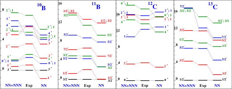
Figure 5: States dominated by p-shell configurations for ¹⁰B, ¹¹B, ¹²C, and ¹³C. From navratil09

5.2 Continuum states

In general, if the reaction implies a state belonging to the continuum spectrum of $\hat{H}$, the challenge may become enormous, since one has to deal with the many–body scattering problem, which may lack a viable solution already for a very small number of constituents in the system. The difficulty in calculating a many–body cross section involving continuum states can be realized, if one considers that, at a given energy, the wave function of the system may have many different components (channels), corresponding to all its partitions into fragments of various sizes. Already in a rather small system of four constituents, at energies beyond the so–called four–body break–up threshold, the two–, the three– and the four–body break–up channels contribute. In configuration space the task consists in finding the solution of the four–body Schrödinger equation with the proper boundary conditions. It is just the implementation of the boundary conditions for a continuum wave function which constitutes the main obstacle to the practical solution of the problem. In fact, the necessary matching of the wave function to the oscillating asymptotic behavior (sometimes even difficult to be defined unambiguously) is not feasible in practice. In momentum space the situation is as complicated. The proper extension of the Lippmann–Schwinger equation to a many–body system has been formulated long ago with the Faddeev–Yakubowski equations FADDEEV:1961 ; YAKUBOWSKY:1967 . However, because of the involved analytical structure of their kernels and the number of equations itself, to date it is impossible to solve the problem directly with their help, at energies above the four–fragment break–up threshold, even for a number of constituents as small as just four.

6 Integral transform methods

Alternative approaches to the quite challenging problem of the dynamics in the continuum are provided by integral transform methods. The Lorentz Integral transform (LIT) method EFROS:1994 is the natural extension of an original idea EFROS:1985 ; LIT_REPORT to calculate reaction cross sections with the help of integral transforms. This kind of approach is rather unconventional. It starts from the consideration that the amount of information contained in the wave function is redundant with respect to the transition matrix elements needed in the cross section. Therefore, one can avoid the difficult task of solving the Schrödinger equation. Instead one can concentrate directly on the matrix elements. With the help of theorems based on the closure property of the Hamiltonian eigenstates, it is proved that these matrix elements (or some combinations of them) can be obtained by a calculation of an integral transform with a suitable kernel, and its subsequent inversion. The main point is that for some kernels the calculation of the transform requires the solution of a Schrödinger–like equation with a source, and that its solutions have asymptotic conditions similar to a bound state. In this sense one can say that the integral transform method reduces the continuum problem to a much less problematic bound–state–like problem.

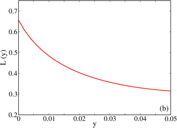
Figure 6: (a): the function $f(x)$; (b): its Laplace transform $L(y)=\int f(x)\exp[-xy]dx$

The form of the kernel in the integral transform is crucial. The reason is that in order to get the quantities of interest the transform needs to be inverted. Since it is normally calculated numerically it is affected by inaccuracies, and inverting an inaccurate transform is somewhat problematic. Actually, when the inaccuracies in the input transform tend to decrease, and a proper regularization is used in the course of inversion, the final result approaches the true one for various kernels TIKHONOV:1977 . However, the quality of the result of the inversion may vary substantially according to the form of the kernels, even for inaccuracies of similar size in the transforms. In particular, when, for a specific kernel, the accuracy of the transform is insufficient, the result may be corrupted with oscillations superimposing the true solution.

In EFROS:1985 the Stieltjes kernel was proposed and its reliability was tested and discussed in simple model studies. Later, in a test of the method on a realistic electromagnetic cross section, calculated also in the conventional way for the deuteron EFROS:1993 , it was found that the use of the Stieltjes kernel is not satisfactory, since it leads to quite inaccurate results. The problem with the Stieltjes kernel can be understood if one notices that its form is not qualitatively different from that of the Laplace kernel. In fact it is well known that the problem of the inversion of a Laplace transform is extremely ill posed when the input is numerically noisy and incomplete  ACTON:1970 . To illustrate the difficulties with the inversion of such kernels consider figure 6. In the upper and lower parts of the figure the function of interest and its Laplace transform are shown, respectively. As one can see the two curves do not resemble each other. The former shows a curve with a bump, the latter a monotonically decreasing curve. If now one thinks that the second may be affected by numerical errors as a result of the calculation one understands how difficult it may be to reconstruct the curve in figure 6(a). The Laplace kernel in fact has spread the information about the curve over a large domain.

Nevertheless the use of Laplace transforms is common in various fields of physics, from condensed matter to lattice QCD, and elaborated algorithms (e.g. the maximum entropy method JAYNES:1978 ) are sometimes employed for its inversion.

The problems encountered in inverting the Stieltjes as well as the Laplace transform has led to the conclusion that, differently from those two cases, the ‘best’ kernel should be of a finite range. Its extension should be, roughly speaking, about the range of the quantity to be obtained as the result of the inversion. Actually the perfect kernel would be a $\delta-$function. In this case in fact the function and its transform would coincide. However, this clearly does not help! However, a so called representation of the $\delta-$function would have the necessary characteristics.

At the same time, however, the transform has to be calculable in practice. In EFROS:1994 it has been found that the Lorentzian kernel satisfies both requisites and the analogous test, as had been performed in EFROS:1993 for the Stieltjes kernel, has led to very accurate results.

6.1 The Lorentz Integral transform (LIT) method

In the inclusive electron scattering process discussed in these lectures the quantity of interest are the response functions $R_{L}$ and $R_{T}$ contained in the cross section. Like any general perturbation induced inclusive reaction (as are the e.w. reactions with hadron systems) they have the following structure

$$r(E)=\sum\!\!\!\!\!\!\!\int\,d\gamma\langle Q|\Psi_{\gamma}\rangle\langle\Psi_{\gamma}|Q^{\prime}\rangle\delta(E_{\gamma}-E)\,,$$ (53)

where $|\Psi_{\gamma}\rangle$ are solutions to the dynamic equation

$$(\hat{H}-E_{\gamma})|\Psi_{\gamma}\rangle=0\,,$$ (54)

and $\hat{H}$ is the Hamiltonian of the system. The set $|\Psi_{\gamma}\rangle$ is assumed to be complete and orthonormal,

$$\sum\!\!\!\!\!\!\!\int\,d\gamma|\Psi_{\gamma}\rangle\langle\Psi_{\gamma}|=1\,.$$ (55)

The integration and summation here and in (53) go over all discrete states and continuum spectrum states in the set.

We suppose that the norms $\langle Q|Q\rangle$ and $\langle Q^{\prime}|Q^{\prime}\rangle$ are finite. One has $|Q\rangle=\hat{O}|\Psi_{0}\rangle$, $|Q^{\prime}\rangle=\hat{O}^{\prime}|\Psi_{0}\rangle$, where $|\Psi_{0}\rangle$ is the initial state in a reaction (generally the ground state of the system undergoing the perturbation), and $\hat{O}$, $\hat{O}^{\prime}$ are transition operators. In the electron scattering case discussed above they are both equal to the charge or to the current operators. Then one has

$$r(E)=\sum\!\!\!\!\!\!\!\int\,d\gamma\langle\Psi_{0}|\hat{O}^{\dagger}|\Psi_{\gamma}\rangle\langle\Psi_{\gamma}|\hat{O}^{\prime}|\Psi_{0}\rangle\delta(E_{\gamma}-E)\,.$$ (56)

Here $|\Psi_{\gamma}\rangle$ is a set of final states.

As already pointed out, when the energy $E$ and the number of particles in the system increase the direct calculation of the quantity $r(E)$ becomes prohibitive. The difficulty is related to the fact that in these cases a great number of continuum spectrum states $|\Psi_{\gamma}\rangle$ contribute to $r(E)$ and the structure of these states is very complicated.

The integral transform approach to overcome this difficulty can be considered as a generalization of the sum rule approach, since the use of the closure property of the Hamiltonian eigenstates plays a fundamental role. Consider for example a simple sum rule for the quantity (56), based on the closure property (55) i.e.

$$\sum\!\!\!\!\!\!\!\int\,r(E)dE=\langle Q|Q^{\prime}\rangle\,.$$ (57)

The calculation of this quantity is much easier than a direct calculation of $r(E)$ itself, since it requires the knowledge of $|Q\rangle$ and $|Q^{\prime}\rangle$ only. This can be obtained with bound–state methods since it was supposed that $|Q\rangle$ and $|Q^{\prime}\rangle$ have finite norms. However, this sum rule contains only a limited information on $r(E)$. In order to get much more information about it we consider instead an integral transform

$$\Phi(\sigma)=\sum\!\!\!\!\!\!\!\int\,K(\sigma,E)\,r(E)\,dE$$ (58)

with a smooth kernel $K$. This yields

$$\Phi(\sigma) = \sum\!\!\!\!\!\!\!\int\,d\gamma\langle Q|\Psi_{\gamma}\rangle K(\sigma,E_{\gamma})\langle\Psi_{\gamma}|Q^{\prime}\rangle$$ (59)

$$= \sum\!\!\!\!\!\!\!\int\,d\gamma\langle Q|\hat{K}(\sigma,\hat{H})|\Psi_{\gamma}\rangle\langle\Psi_{\gamma}|Q^{\prime}\rangle\,.$$

Using the closure property (55) one obtains

$$\Phi(\sigma)=\langle Q|\hat{K}(\sigma,\hat{H})|Q^{\prime}\rangle\,.$$ (60)

Therefore equation (60) may be viewed as a generalized sum rule depending on a continuous parameter $\sigma$. Only with a proper choice of the kernel $K$ the right–hand side of (60) may be calculated using bound–state type methods. And, as it was already said, even if $\Phi(\sigma)$ is available (58) may not always be solved with enough accuracy to obtain $r(E)$ via an inversion of the transform.

Our choice of the kernel $K(\sigma,E)$ is such that both the calculation of $\Phi(\sigma)$ and the inversion of (58) are feasible. We choose EFROS:1994

$$K(\sigma,E)=\frac{1}{(E-\sigma^{*})(E-\sigma)}\,.$$ (61)

Notice that the energy parameters $\sigma$ that we consider are complex. For convenience we define them as

$$\sigma=E_{0}+\sigma_{R}+i\sigma_{I}\,,$$ (62)

where $E_{0}$ is the ground–state energy, and $\sigma_{I}\neq 0$, so that $K(\sigma,E)$ is actually a Lorentzian function centered on $E_{0}+\sigma_{R}$, having $\sigma_{I}$ as a half width

$$K(\sigma_{R},\sigma_{I},E)=\frac{1}{(E-E_{0}-\sigma_{R})^{2}+\sigma_{I}^{2}}\,.$$ (63)

Then the integral transform (58) becomes

$$L(\sigma_{R},\sigma_{I})=\sum\!\!\!\!\!\!\!\int\,dE\,\frac{r(E)}{(E-E_{0}-\sigma_{R})^{2}+\sigma_{I}^{2}}\,.$$ (64)

Here and in the following the integral transform $\Phi(\sigma)$ with a Lorentz kernel is denoted by $L(\sigma_{R},\sigma_{I})$. Using the definition (56) it is easy to show that the quantity (64) may be represented as

$$L(\sigma_{R},\sigma_{I})=\langle\tilde{\Psi}|\tilde{\Psi}^{\prime}\rangle\,,$$ (65)

where the ‘LIT functions’ $\tilde{\Psi}$ and $\tilde{\Psi}^{\prime}$ are given by

$$|\tilde{\Psi}\rangle = \left(\hat{H}-E_{0}-\sigma_{R}-i\sigma_{I}\right)^{-1}\hat{O}|\Psi_{0}\rangle\,,$$ (66)

$$|\tilde{\Psi}^{\prime}\rangle = \left(\hat{H}-E_{0}-\sigma_{R}-i\sigma_{I}\right)^{-1}\hat{O}^{\prime}|\Psi_{0}\rangle\,.$$ (67)

These functions are solutions to the inhomogeneous equations

$$\left(\hat{H}-E_{0}-\sigma_{R}-i\sigma_{I}\right)|\tilde{\Psi}\rangle = \hat{O}|\Psi_{0}\rangle\,,$$ (68)

$$\left(\hat{H}-E_{0}-\sigma_{R}-i\sigma_{I}\right)|\tilde{\Psi}^{\prime}\rangle = \hat{O}^{\prime}|\Psi_{0}\rangle\,.$$ (69)

When $\hat{O^{\prime}}=\hat{O}$, $L(\sigma)$ equals to $\langle\tilde{\Psi}|\tilde{\Psi}\rangle$. Since for $\sigma_{I}\neq 0$ the integral in (64) does exist, the norm of $|\tilde{\Psi}\rangle$ is finite. This implies that $|\tilde{\Psi}\rangle$ is a localized function. Consequently, (68) can be solved with bound–state type methods. Similar to the problem of calculating a bound state it is sufficient to impose the only condition that the solutions of (68) is localized. This means that in contrast to continuum spectrum problems, in order to construct a solution, it is not necessary here to reproduce a complicated large distance asymptotic behavior in the coordinate representation or singularity structure in the momentum representation. This is a very substantial simplification.

Obviously, localized solutions to (68) and (69) are unique. Once $L(\sigma)$ is calculated $r(E)$ is obtained by inversion of the integral transform with a Lorentzian kernel (64) (‘Lorentz integral transform’). The inversion of the LIT is discussed in the following.

6.2 The inversion of the transform

As already pointed out, the main advantage of the LIT method to study reactions is that one avoids to solve the many–body scattering problem. One solves instead, with bound–state methods, equations of the form (68). The knowledge of those solutions leads to the LIT of the function $r$ of interest. A crucial part of the method is then the inversion of this integral transform. The inversion of this integral transform has to be made with care, since errors in the transform can generate oscillations. To illustrate this let us consider a well defined $r(E)$ to which we add a high-frequency term $\Delta^{\Omega}r(E)$. The latter leads to an additional $\Delta L^{\Omega}(\sigma_{R},\sigma_{I})$ in the transform. For any amplitude of the oscillation $\Delta^{\Omega}L$ decreases with increasing $\Omega$. This means that for some value of $\Omega$ $\Delta^{\Omega}L$ may be smaller than the size of the errors in the calculation. Therefore in this case $\Delta^{\Omega}r$ cannot be discriminated. By reducing the error in the calculation one can push the frequency of the undiscriminated $\Delta\Omega r$ to higher and higher values.

One of the methods that can be adopted to invert the transform is called the regularization method TIKHONOV:1977 . This has led to very safe inversion results. Alternative inversion methods are discussed in ANDREASI:2005 . They can be advantageous in case of response functions with more complex structures. Up to now, however, such complex structures have not been encountered in actual LIT applications, since the various considered $r(e)$ have normally (i) a rather simple structure, where essentially only a single peak of $r(e)$ has to be resolved, or (ii) a more complicated structure, which however can be subdivided into a sum of simply structured responses, where the various LITs can be inverted separately. The present ‘standard’ LIT inversion method consists in the following ansatz for the response function

$$r(e^{\prime})=\sum_{n=1}^{N_{max}}c_{n}\chi_{n}(e^{\prime},\alpha_{i})\,,$$ (70)

with $e^{\prime}=e-e_{th}$, where $e_{th}$ is the threshold energy for the break–up into the continuum. The $\chi_{n}$ are given functions with nonlinear parameters $\alpha_{i}$. A basis set frequently used for LIT inversions is

$$\chi_{n}(\epsilon,\alpha_{i})=\epsilon^{\alpha_{1}}\exp(-{\frac{\alpha_{2}\epsilon}{n}})\,.$$ (71)

In addition also possible information on narrow levels could be incorporated easily into the set $\chi_{n}$. Substituting such an expansion into the right hand side of (64) (here too the $\sigma_{I}$ dependence is omitted) one obtains

$$L(\sigma_{R})=\sum_{n=1}^{N_{max}}c_{n}\tilde{\chi}_{n}(\sigma_{R},\alpha_{i})\,,$$ (72)

where

$$\tilde{\chi}_{n}(\sigma_{R},\alpha_{i})=\int_{0}^{\infty}de^{\prime}{\frac{\chi_{n}(e^{\prime},\alpha_{i})}{(e^{\prime}-\sigma_{R})^{2}+\sigma_{I}^{2}}}\,\,.$$ (73)

For given $\alpha_{i}$ the linear parameters $c_{n}$ are determined from a least–square best fit of $L(\sigma_{R})$ of equation (72) to the calculated $L(\sigma_{R})$ of equation (65) for a number of $\sigma_{R}$ points much larger than $N_{max}$.

For every value of $N_{max}$ the overall best fit is selected and then the procedure is repeated for $N^{\prime}_{max}=N_{max}+1$ till a stability of the inverted response is obtained and taken as inversion result. A further increase of $N_{max}$ will eventually reach a point, where the inversion becomes unstable leading typically to random oscillations. The reason is that $L(\sigma_{R})$ of equation (72) is not determined precisely enough so that a randomly oscillating $r(e)$ leads to a better fit than the true response. If the accuracy in the determination of $L(\sigma_{R})$ from the dynamic equation is increased then one may include more basis functions in the expansion (72).

The LIT method has to be understood as an approach with a controlled resolution. If one expects that $r(E)$ has structures of width $\gamma$ then the LIT resolution parameter $\sigma_{I}$ should be similar in size. Then it is sufficient to determine the corresponding LIT with a moderately high precision, and the inversion should lead to reliable results for $r(E)$ if in fact no structures with a width smaller than $\Gamma$ are present. If, however, there is a reason to believe that $r(E)$ exhibits such smaller structures one should reduce $\sigma_{I}$ accordingly and perform again a calculation of $L$ with the same relative precision as before. Such a calculation is of course more expensive than the previous one with larger $\sigma_{I}$, but in principle one can reduce the LIT resolution parameter $\sigma_{I}$ more and more. The advantage of the LIT approach as compared with a conventional approach is evident. In the LIT case one makes the calculation with the proper resolution, while in a conventional calculation an infinite resolution (corresponding to $\sigma_{I}=0$) is requested, which often makes such a calculation not feasible.

There are several tests of the reliability of the inversion. First of all, performing the calculation at different $\sigma_{I}$ one has to obtain the same stable result. If $\sigma_{I}$ is too small the solution tends very slowly to zero, therefore for $\sigma_{I}\geq\sigma_{I}^{min}$ one may have numerical problems, turning into large errors for the LIT. As already said above, this will show up in unphysical oscillations in $r(E)$. This means that the stable result obtained with $\sigma_{I}<\sigma_{I}^{min}$ is the correct one, at that resolution. Another test is the control of the moments, in fact the moments of $r(E)$ can be calculating both integrating $r(E)$ or by expression (60) (with $K(\sigma,H)=H^{\sigma}$ and $\sigma$ integer), which needs only the bound state.

6.3 Practical calculation of the LIT

We have seen how the LIT method reformulates a scattering problem as a Schrödinger–like equation with source terms which depend on the kind of reaction under consideration. These equations, which we will call the ‘LIT equations‘ are essentially the same for any reaction, differing by the source term i.e. by their right hand side (see (68), (69)). In all cases the asymptotic boundary conditions are bound–state–like. Consequently the solutions of these equations can be found with similar methods as for the bound–state wave functions.

As we have seen above bound state solutions of the Schrödinger equation can be found in different ways searching for a direct numerical solution of the differential equations in coordinate space (or of the integro–differential equations in momentum space), or alternatively using expansions on some basis set of localized functions (bound-state-like boundary condition). These expansion methods become more and more advantageous with respect to the former one, with increasing particle number. For this reason, and because it has been used for the vast majority of the LIT applications I discuss it in the following. The truncation of the basis set converts the bound–state Schrödinger equation into a matrix eigenvalue problem and the LIT equations into a set of linear equations. These equations can be solved with various iteration methods and also Gauss type non–iteration ones. Such strategies have the drawback that one should solve these equations many times, as many as the number of $\sigma_{R}$ values that one needs for a proper inversion of the transform. There are, however, two better strategies for calculating $L(\sigma)$. The first strategy, which is called the eigenvalue method involves the full diagonalization of the Hamiltonian matrix and expresses the LIT through its eigenvalues. This method is instructive from a theoretical point of view.

Regardless of the reaction under consideration and the process that one wants to study the LIT method requires the calculation of the overlap (see (65)–(67))

$$L(\sigma_{R},\sigma_{I}) = \langle\tilde{\Psi}|\tilde{\Psi}^{\prime}\rangle$$ (74)

$$= \langle Q|\frac{1}{(\hat{H}-E_{0}-\sigma_{R}+i\sigma_{I})}\frac{1}{(\hat{H}-E_{0}-\sigma_{R}-i\sigma_{I})}|Q^{\prime}\rangle\,,$$

where $|Q^{\prime}\rangle$ and $|Q\rangle$ contain the information about the kind of reaction one is considering. Seeking $|\tilde{\Psi}\rangle$ and $|\tilde{\Psi}^{\prime}\rangle$ as expansions over $N$ localized basis states, it is convenient to choose as basis states $N$ linear combinations of states that diagonalize the Hamiltonian matrix. Let’s denote these combinations $|\varphi_{\nu}^{N}\rangle$ and the eigenvalues $\epsilon_{\nu}^{N}$. The index $N$ is to remind that they both depend on $N$. If the continuum starts at $E=E_{th}$ then at sufficiently high $N$ the states $|\varphi_{N}\rangle$ having $\epsilon_{\nu}^{N}<E_{th}$ will represent approximately the bound states. The other states will gradually fill in the continuum as $N$ increases. The expansions of our localized LIT functions read as

$$|\tilde{\Psi}\rangle=\sum_{\nu}^{N}\frac{\langle\varphi_{\nu}^{N}|Q\rangle}{\epsilon_{\nu}^{N}-E_{0}-\sigma_{R}-i\sigma_{I}}|\varphi_{\nu}^{N}\rangle\,,$$ (75)

$$|\tilde{\Psi}^{\prime}\rangle=\sum_{\nu}\frac{\langle\varphi_{\nu}^{N}|Q^{\prime}\rangle}{\epsilon_{\nu}^{N}-E_{0}-\sigma_{R}-i\sigma_{I}}|\varphi_{\nu}^{N}\rangle\,.$$ (76)

Substituting (75) and (76) into (74) yields the following expression for the LIT,

$$L(\sigma_{R},\sigma_{I})=\sum_{\nu}\frac{\langle Q|\varphi_{\nu}^{N}\rangle\langle\varphi_{\nu}^{N}|Q^{\prime}\rangle}{(\epsilon_{\nu}^{N}-E_{0}-\sigma_{R})^{2}+\sigma_{I}^{2}}\;,$$ (77)

and for $|Q^{\prime}\rangle=|Q\rangle$

$$L(\sigma_{R},\sigma_{I})=\sum_{\nu}\frac{|\langle\varphi_{\nu}^{N}|Q\rangle|^{2}}{(\epsilon_{\nu}^{N}-E_{0}-\sigma_{R})^{2}+\sigma_{I}^{2}}\;.$$ (78)

From (77) and (78) it is clear that $L(\sigma_{R},\sigma_{I})$ is a sum of Lorentzians. The inversion of the LIT contributions from the states with $\epsilon_{\nu}^{N}<E_{th}$ gives the discrete part of a response function, whereas the inversion of the rest gives its continuum part. The spacing between the corresponding eigenvalues with $\epsilon_{\nu}^{N}>E_{th}$ depends on $N$ and in a given energy region the density of these eigenvalues increases with $N$. (Since the extension of the basis states grows with $N$, this resembles the increase of the density of states in a box, when its size increases.)

The second strategy to obtain the LIT utilizes the Lanczos algorithm LANCZOS:1950 ; GOLUB:1983 expressing the LIT as a continuous fraction. It turns out that for obtaining an accurate LIT only a relatively small number of Lanczos steps are needed. As the number of particles in the system under consideration increases the number of basis states grows up very rapidly and the Lanczos approach seems at present the only viable method to calculate the LIT.

The motivation to use the Lanczos approach comes from the observation that from the computational point of view the calculation of the LIT is much more complicated and demanding than finding the ground state wave function of an $A$–particle system. In fact, to obtain the ground–state wave function one needs only to find the lowest eigenvector of the Hamiltonian matrix. On the contrary, as it is clear from (77) and (78), the complete spectra of $\hat{H}$ over a wide energy range should be known to calculate the LIT. Therefore it is no surprise that the computational time and the memory needed to calculate $L(\sigma)$ have been the limiting factors in extending the LIT method for systems with more than four particles. It turns out that these obstacles can be overcome if the LIT method is reformulated using the Lanczos algorithm. Following reference MARCHISIO:2003 , in this section it is shown how this can be done.

To this end it is assumed that the source states $|Q\rangle$ and $|Q^{\prime}\rangle$ are real and rewrite the LIT in the following form

$$L(\sigma)=-\frac{1}{\sigma_{I}}\mbox{Im}\left\{\langle Q|\frac{1}{\sigma_{R}+i\sigma_{I}+E_{0}-\hat{H}}|Q^{\prime}\rangle\right\}\>\mbox{.}$$ (79)

A similar relation connects the response function $r(e)$ to the Green’s function

$$r(e)=-\frac{1}{\pi}\mbox{Im}\left\{\lim_{\eta\to 0}G(e+i\eta+E_{0})\right\}\>;\hskip 17.07164ptG(z)=\langle Q|\frac{1}{z-\hat{H}}|Q^{\prime}\rangle\>,$$ (80)

provided that $z=e+i\eta$ is replaced by $\sigma_{R}+i\sigma_{I}$. This is not surprising since the properly normalized Lorentzian kernel is one of the representations of the $\delta$–function and $\sigma_{I}/\pi\,L(\sigma_{R})\rightarrow r(\sigma_{R})$ for $\sigma_{I}\rightarrow 0$. In condensed matter calculations DAGOTTO:1994 ; HALLBERG:1995 ; KUEHNER:1995 the Lanczos algorithm has been applied to the calculation of the Green function with a small value of $\eta$, and its imaginary part has been interpreted as $r(e)$ directly. This can be done if the spectrum is discrete (or discretized) and $\eta$ is sufficiently small. In our case we have a genuine continuum problem and we want to avoid any discretization, therefore we calculate $L(\sigma_{R})$ in the same way, i.e. with finite $\sigma_{I}$ using the Lanczos algorithm, but then we anti-transform $L(\sigma_{R})$ in order to obtain $r(e)$.

7 application of the LIT method to electroweak response functions

In this section I present some selected results obtained with the LIT method for both the electron scattering response functions and the photoabsorption cross section. In the various cases the LIT equation (68) has been solved with different ab initio bound state methods. For A$\geq 4$ the most efficient one has turned out to be the EIHH method Barnea00 ; Barnea01 , which, till now, has allowed to reach results up to A=7.

The selection of reselts presented in the following is done with two scopes: the first is to illustrate how from the comparison between theoretical ab initio results and experimental data one can get information on the nuclear force. The second is to show how, when A increases, a microscopic calculation can give rise to macroscopic features, giving the possibility to study the link between the two scales (see the case A=6).

However, before entering into that discussion it is worth showing how the LIT method is working in systems where the direct calculation of continuum states is possible. This is the case of the two-body system, i.e. the deuteron.

7.1 Results for A=2

The very first LIT application was the calculation of the deuteron longitudinal form factor $R_{L}(q,\omega)$ at $|\vec{q}|=440$ MeV/c in  EFROS:1994 , where the LIT has been originally proposed. Actually it served as a test case for the applicability of the LIT approach, since one can calculate $np$ continuum state wave functions explicitly. There it was shown how good was the agreement between the responses obtained in the two ways. Here another example on the total deuteron photodisintegration is shown.

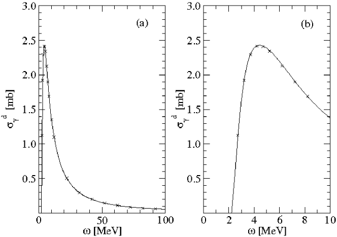
Figure 7: Total deuteron photoabsorption cross section up to 100 MeV (a) and 10 MeV (b): LIT result (solid) and from calculation with explicit np final state wave function (crosses).

Figure 7 shows the comparison of the LIT result with that of the conventional calculation, using the proper np scattering states. Also here one observes an excellent agreement between the two calculations, showing the high precision that can be obtained with the LIT method.

At this point let us make a digression about the operator which is very often used in the photoabsorption calculations, i.e. the dipole operator $D_{z}=\sum_{i}z_{i}\tau_{i}^{3}$. Let us briefly explain why one uses such an operator in the (low energy) photoabsorption cross section.

The photoabsorption cross section can be obtained by the electron scattering one in the limit $Q^{2}=0$ ($|\vec{q}|=\omega$). This means that the longitudinal part of the cross section disappears (the photon has no charge). Therefore one remains with the part where the transverse current operator is present (the photon fields are transverse to $\vec{q}$). If one makes a multipole expansion of the current operator and works out the cumbersome formulas, at some point one realizes that there are terms that contain the $\vec{\nabla}\cdot\hat{\vec{J}}$. This is nice because, at least for these terms, it is possible to use the continuity equation again, avoiding the knowledge of the current. So one can connect these terms to the charge density multipoles. The interesting fact is that the remaining terms are of higher order in $|\vec{q}|$ and therefore can be neglected if $|\vec{q}|$, (i.e. $\omega$) is small enough. However, if $\omega$ is small enough, one can also neglect all the multipoles higher than the first, i.e. one remains with the dipole. This is what is called Siegert Theorem. The great importance of this theorem is the fact that one can avoid to know $\hat{\vec{J}}$ ! The information about it is intrinsically contained in the use of the dipole operator. For our scope this has a very important consequence: if we use a phenomenological potential in the calculation, the comparison theory-experiment will tell us whether the unknown implicit degrees of freedom, implied by it, are the right ones.

7.2 Results for A=3

For the 3-body problem in the continuum one can solve the Faddeev equations and calculate continuum states both in the two- and three-body break up channels. Therefore also in this case one can benchmark traditional results with those obtained by the LIT. This has been done in martinelli ; bench3 . Reference martinelli is interesting because there the LIT equation has been solved translating it into the Faddeev scheme, showing once more that it can be solved with different techniques. The excellent result of the benchmark from bench3 is reported in figure 8.

Figure 8: Comparison of the Faddeev and LIT results for the total ³H photoabsorption cross section. The dots are the Faddeev results and the two curves represent the bounds for the inversion of the LIT. From bench3

Notice that in the figure the small uncertainty due to the inversion is also shown.

Now I am going to illustrate an instructive example, taken from references MEKLOTY and 3RTAV18 , of how one gets information about the subnuclear d.o.f. from the calculation of $R_{T}$. In MEKLOTY the Bonn potential BonnRA , which is a potential based on meson theory was used, while in 3RTAV18 the potential was the phenomenological AV18 AV18 . Therefore in the former case the currents are known, while in the latter a recipe is proposed in order to construct them so that their divergence is consistent with the potential via the continuity equation. However, only the comparison with data can say whether they are correct. In analogy with the one boson exchange potential case these currents are called meson exchange currents and indicated by MEC. Figure 9 illustrates the importance of these MEC and the quality of the comparison with existing data.

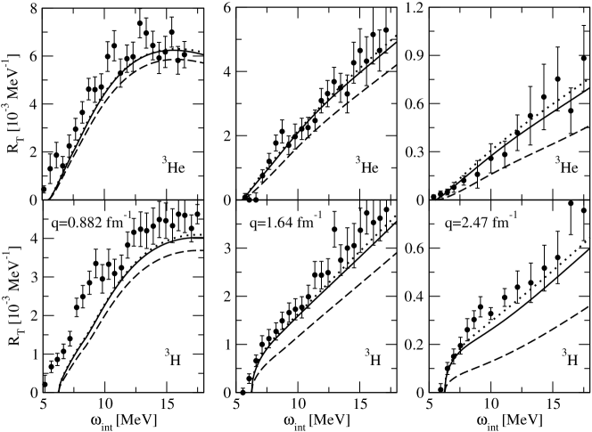
Figure 9: Comparison of experimental and theoretical results for the threshold ³He (upper panels) and ³H (lower panels) transverse response function RT as function of internal excitation energy !int at three momentum transfers q. Theoretical results with different current operators: relativistic one-body current (dashed), relativistic one-body current + MEC (solid), non-relativistic one-body current + MEC (dotted). Experimental data from Retzlaff .

In case of ³He one has a rather good agreement of theoretical and experimental transverse response functions for the two higher $|\vec{q}|$ values. The MEC contribution is essential for reaching this agreement. At $|\vec{q}|$ = 0.88 fm^-1, however, the theoretical $R_{T}$ underestimates the data below 11 MeV. In the triton case the situation looks worse. Already for the two higher $|\vec{q}|$ values one finds a slight underestimation of the data, in addition the discrepancy becomes even larger at the lowest $|\vec{q}|$. One can conclude that the present agreement between theory and experiment is not bad, but certainly not very good. The interesting point is that it seems that a different nuclear force does not improve the situation, since the results at $|\vec{q}|$ = 0.88 fm^-1 with the BonnA potential from MEKLOTY is almost identical to the AV18 result (the ³H case was not considered in MEKLOTY ). Additional currents involving the $\Delta$ resonance, up to now only partially considered in the literature for the threshold kinematics, could probably lead to a small improvement.

7.3 Results for A=4

Among light nuclei the $\alpha$-particle (⁴He) is of particular importance because it has some typical features of heavier systems (e.g. binding energy per nucleon), which make it a precious link between the classical few-body systems, i.e. deuteron, triton and ³He, and more complex nuclei. For example in ⁴He one can study the possible emergence of collective phenomena typical of complex nuclei like the giant dipole resonance (GDR). This is the famous bump which is seen in the total photoabsorption cross section of all nuclei and that has been interpreted as a collective oscillating motion of the protons against the neutrons. Furthermore ⁴He is the ideal testing ground not only for the NN potential but also for the multi-nucleon forces and in particular of the three-body force (3BF).

7.3.1 Digression on the three-body force

As was already remarked above, the nuclear potential has clearly an effective nature, therefore it is in principle a many-body operator. Yet the debate has concentrated for several decades only on the two-body part. Such a debate has taken place essentially among three different points of view: those based on meson theory, purely phenomenological ones and more recently the point of view of effective field theory. Realistic potentials based on all three different approaches have been constructed, relying on fits to thousands of N-N scattering data. After that precise calculations of the triton binding energy have demonstrated that a two-body potential is not enough to explain the experimental value, the same debate is taking place regarding three-body forces. However, for the determination of a realistic three-body potential or to discriminate among different models one needs to find A$\geq 3$ observables that are sensitive to it. One direction that has been followed wiringa04 ; wiringa00 is to calculate accurately bound properties of nuclei of increasing A. In fact it has been realized that stronger and stronger discrepancies exist between the binding energies calculated with high precision two-body potentials and the experimental values (see the upper part of figure 4). Another very promising direction is to study electromagnetic reactions in the continuum. In fact many years of electron scattering experiments have demonstrated the power of this kind of reactions, and in particular of the inelastic ones, because of the possibility to vary energy $\omega$ and momentum $|\vec{q}|$ transferred by the electron to the nucleus. This allows one to focus on different dynamical aspects at different ranges and one might find regions where the searched three-body effects are sizable.

The ⁴He nucleus is particularly appropriate for these studies because of the following considerations: i) the ratio between the number of triplets and of pairs goes like $(A-2)/3$, therefore it is double for ⁴He than for ³He; ii) theoretical results on hadron scattering observables involving four nucleons deltuva as well as ⁴He-N phase shifst sofiascattering seem to imply that three-body effects are rather large.

Digression on the experimental situation

In order to appreciate the importance of the theoretical results presented in the following it is necessary to summarize the situation of the experiments regarding electromagnetic reactions on ⁴He.

Let us start from the real photon case, which has has a longstanding history. First experiments on the $(\gamma,n)$ reaction were performed about fifty years ago. In the following twentyfive years various experimental groups carried out measurements for both the $(\gamma,p)$and $(\gamma,n)$ reaction channels and the inverse capture reactions Dramatically conflicting results have been obtained as a result of this work. The $(\gamma,p)$ data were consistent in showing a rather pronounced resonant peak close to the three-body breakup threshold. At the same time, the $(\gamma,n)$ data at low energy were very spread, and measurements showed either a strongly pronounced or a rather suppressed giant dipole peak. In 1983 a careful and balanced review of all the available experimental data for the two mirror reactions was provided CBD:1983 . A strongly peaked cross section at low energy for the ($\gamma,p$) channel and a flatter shape for the ($\gamma,n$) one was recommended by the authors. Three new experiments on the ($\gamma,p$) reaction were subsequently carried out, two of them contradicting and one confirming the recommended cross section. Measurements of the ratio of the $(\gamma,p)$ to $(\gamma,n)$ cross sections in the giant resonance region were performed as well FLORIZONE94 and, at variance with the cross sections recommended in CBD:1983 , results very close to unity were reported. Finally, in 1992 additional cross section data were deduced from a Compton scattering experiment on ⁴He Wells92 . A strongly peaked cross section for the ⁴He total photoabsorption was found suggesting a ($\gamma,n$) cross section considerably larger than the one recommended in CBD:1983 .

In 1996 the first theoretical calculation of the two-fragment breakup cross section with inclusion of FSI was performed in the energy range below the three-fragment breakup threshold Ell96 . The semi-realistic MTI-III potential MT69 was employed. The results of Ell96 showed a rather suppressed giant dipole peak. The agreement with the ($\gamma$,n) data in Berman was very good and the situation seemed to be settled.

However, the following year a calculation of the total photoabsorption cross section for the ⁴He up to the pion threshold was carried out ELO97 . Full FSI was taken into account in the whole energy range via the application of the LIT method. The four-nucleon dynamics was described with the same NN potential as in Ell96 . Different from the previous work a pronounced giant dipole peak was found. These results have been reexamined in BELO01 ; Sofia1 . A small shift of the peak position has been obtained, but the pronounced peak has been confirmed.

Unfortunately, the experimental situation of the ⁴He photodisintegration is not yet sufficiently settled. Most of the experimental work has concentrated on the two-body break-up channels ⁴He$(\gamma,n)^{3}$He and ⁴He$(\gamma,p)^{3}$H in the giant resonance region, but still today there is large disagreement in the peak. In fact in two recent $(\gamma,n)$ experiments Lund ; Shima one finds differences of a factor of two. A measurement of the analog of the GDR in ⁴He has been performed in NAKAYAMA07 via the ⁴He(⁷Li,⁷Be) and points to a cross section which is very close to the result in ELO97 .

Considering that from the early times of atomic physics the cross section for absorption of photons has always represented the fundamental observable to study the spectrum of composite systems, the present situation is unacceptable. Therefore it is highly desirable that this observable attracts the interest of experimentalists. (Projects in this direction have been recently considered at MaxLab in Lund and HI$\gamma$S at TUNL in North Carolina).

Regarding the experimental situation for electron scattering, in the ’80 and ’90’s an intense experimental activity has been devoted to it, in particular to inclusive electron scattering (denoted by $(e,e^{\prime})$) in the so called quasi-elastic (q.e.) regime, corresponding to momentum transfers of several hundreds MeV/c and energies around the q.e. peak, observed at about $q^{2}/2m$. In such conditions one can envisage that the electron has scattered elastically with a single nucleon of mass $m$. Various nuclear targets have been considered, from very light to heavy ones. The reason for concentrating on the q.e. regime has been the conviction that for such kinematics the plane wave impulse approximation (PWIA) might be a reliable framework to describe the reaction. The neglect of the final state interaction (FSI) has the advantage to allow a simple interpretation of the cross section in terms of the dynamical properties of the nucleons in the ground state. In particular the focus in those years were the ground state short range correlations, i.e. the dynamical effects on the wave function of the largely unknown repulsive short range part of the potential.

It is clear, however, that it is important to clarify the reliability of the PWIA. As it will be seen in the following, the LIT method, which takes into account the full dynamics in the final state, allows to clarify this issue.

The comparison theory-experiment for the photon case

An important step forward on the theory side has been made by performing a calculation of the total photoabsorption cross section $\sigma_{\gamma}$ of ⁴He with a realistic nuclear force PRLPhoton . To this end the four-body problem with the Argonne V18 (AV18) NN potential AV18 and the Urbana IX (UIX) 3NF AV18+ has been solved. The results are shown in figure 10.

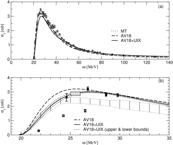
Figure 10: Total ⁴He photoabsorption cross section: (a) $\sigma_{\gamma}$ (AV18) and $\sigma^{\infty}_{\gamma,19}$ (AV18+UIX), (b) as (a) but also included upper/lower bounds and various experimental data (see text), area between dotted lines Berman ; Feldman , dotted box Wells92 , squares Lund , and circles Shima .

Due to the 3NF one observes a reduction of the peak height by about 6% and a shift of the peak position by about 1 MeV towards higher energy. Large effects of the 3NF are found above 50 MeV with an increase of $\sigma_{\gamma}$ by e.g. 18%, 25%, and 35% at $\omega=60$, 100, and 140 MeV, respectively. It is very interesting to compare the present 3NF effects to those found for $\sigma_{\gamma}(^{3}$H/³He) ELOT00 ; bench3 . Surprisingly, the peak height reduction is smaller for ⁴He. For ³H/³He the size of the reduction is similar to the increase of $E_{b}$ (10%), whereas for ⁴He the 3NF increases $E_{b}$ by 17%, but reduces the peak by only 6% and thus cannot be interpreted as a simple binding effect. Also at higher $\omega$ there are important differences. The enhancement of $\sigma_{\gamma}(^{4}$He) due to the 3NF is significantly stronger, namely about two times larger than for the three-body case. Interestingly this reflects the above mentioned different ratios between triplets and pairs in three- and four-body systems. In figure 10(a) also $\sigma_{\gamma}$ for the semi-realistic Malfliet-Tjon (MT) NN potential ELO97 ; BELO01 is illustrated. Similar to $\sigma_{\gamma}(^{3}$H/³He) ELOT00 one finds a rather ”realistic” result in the giant resonance region (overestimations of the peak by about 10-15%) and quite a correct result for the peak position; however, at higher energy $\sigma_{\gamma}$ is strongly underestimated, for ⁴He by a factor of three at pion threshold. In figure 10(a) data from Ark are also shown. They are the only measurements of $\sigma_{\gamma}(^{4}$He) in the whole energy range up to pion threshold. In the peak region the data agree best with the MT potential, while for the high-energy tail one finds the best agreement with the AV18 potential.

In figure 10(b) our low-energy results are compared to further data. which, however have to be interpreted with some care, since no of them corresponds to a direct measurement of the total photoabsorption cross section: (i) in Wells92 the peak cross section is determined from Compton scattering via dispersion relations, (ii) the dashed area corresponds to the sum of cross sections for $(\gamma,n)$ from Berman and $(\gamma,p)^{3}$H from Feldman as already shown in ELO97 , (iii) the data from the above mentioned recent $(\gamma,n)$ experiment Lund are included only up to about the three-body break-up threshold, where one can rather safely assume that $\sigma_{\gamma}\simeq 2\sigma(\gamma,n)$ (see also Sofia1 ), (iv) in Shima all open channels are considered. One sees that the various data are quite different exhibiting maximal deviations of about a factor of two. The theoretical $\sigma_{\gamma}$ agrees quite well with the low-energy data of Berman ; Feldman . In the peak region, however, the situation is very unclear. There is a rather good agreement between the theoretical $\sigma_{\gamma}$ and the data of Lund and Wells92 , while those of Berman ; Feldman are noticeably lower. Very large discrepancies are found in comparison to the recent data of Shima et al. Shima , while a very good agreement is found with data in NAKAYAMA07 .

From all this long discussion it is evident that the experimental situation is rather unsatisfactory and further improvement is urgently needed, if one wants to clarify the 3NF issue. In particular it is worth to stress that due to the above mentioned Siegert’s theorem what one is testing here are also three-body exchange currents connected to the 3NF.

The comparison theory-experiment for the electron case

Inelastic electron scattering off nuclei provides complementary informations on the nuclear dynamics. In fact varying the momentum $|\vec{q}|$, transferred by the electron to the nucleus, one can focus on different dynamical regimes. At lower momenta the collective behavior of nucleons is studied. As $|\vec{q}|$ increases one probes properties of the single nucleon in the nuclear medium and its correlations to other nucleons from long- to short-range. Since the longitudinal response $R_{L}$ is not sensitive to meson exchange effects (only at lowest relativistic order in the Foldy-Wouthuysen transformation) the use of a simple one-body density operator allows to concentrate on the nuclear dynamics generated by the potential and one might find regions where the searched three-nucleon effects are sizable.

Here results on $R_{L}$ are presented, focusing on the evolution of dynamical effects as the momentum transfer decreases. In figures 11 and 12, $R_{L}$ at constant $|\vec{q}|=200$ and 100 MeV/c are shown.

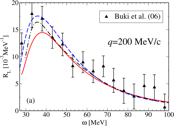
Figure 11: Longitudinal response function for $|\vec{q}|=200$ MeV/c with the AV18 (dashed), AV18+UIX (solid) and MT (dashed-dotted) potentials. Data from Buki06 .

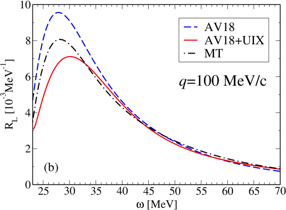
Figure 12: Longitudinal response function for $|\vec{q}|=100$ MeV/c with the AV18 (dashed), AV18+UIX (solid) and MT (dashed-dotted) potentials.

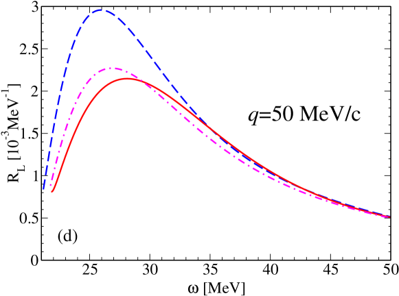
Figure 13: Longitudinal response function for $|\vec{q}|=100$ MeV/c with the AV18 (dashed), AV18+UIX (solid) and MT (dashed-dotted) potentials.

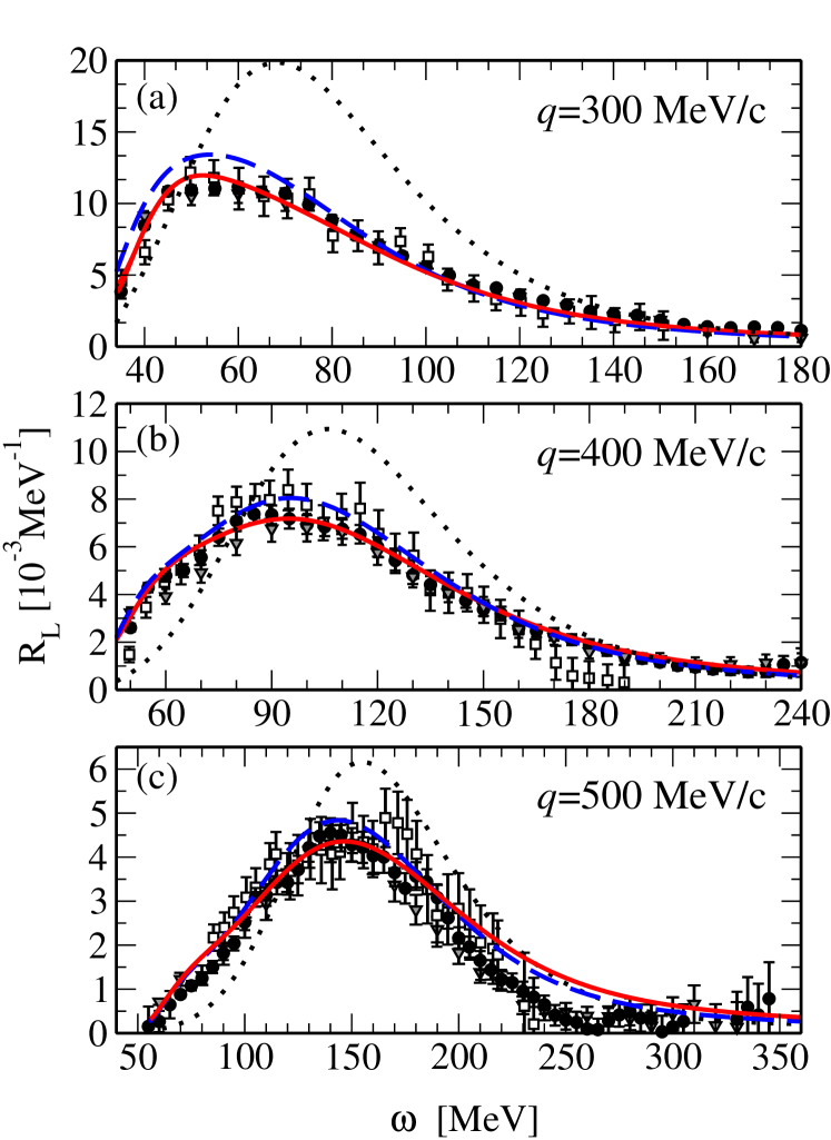
Figure 14: $R_{L}(\omega,q)$ at various $|\vec{q}|$: PWIA (dotted); full calculation with AV18 (dashed) and AV18+UIX (solid). Data from Bates Bates (squares), Saclay Saclay (circles) and world-data set from SICK (triangles).

One has a large quenching effect due the 3NF, which is strongest at lower $|\vec{q}|$. One should notice that such an effect is not simply correlated to the under-binding of the AV18 potential. In fact, if this was the case, the results with the Malfliet-Tjon potential (MT) MT69 , which gives a slight over-binding of ⁴He, would lay even below those obtained with AV18+UIX. On the contrary the MT curve is situated between the curves with and without 3NF.

Given the large 3NF effect at lower $|\vec{q}|$ it is interesting to see whether there is a dependence of the results on the 3NF model itself, investigating in addition other low-q values. To this end the calculation has been performed using also the Tucson Melbourne (TM’) TMprime three-nucleon force at $|\vec{q}|$ = 50 MeV/c. While the UIX force contains a two-pion exchange and a short range phenomenological term, with two 3NF parameters fitted on the triton binding energy and on nuclear matter density (in conjunction with the AV18 two-nucleon potential), the TM’ force is not adjusted in this way. It includes two pion exchange terms where the coupling constants are taken from pion-nucleon scattering data consistently with chiral symmetry. Figure 13 shows that the increase of 3NF effects with decreasing $|\vec{q}|$ is confirmed. Moreover it becomes evident that also the difference between the results obtained with two 3NF models is sizable. One actually finds that the shift of the peak to higher energies in the case of UIX generates for $R_{L}$ a difference up to about 10% on the left hand sides of the peaks. This is a very interesting result. It represents the first case of an electromagnetic observable considerably dependent on the choice of the 3NF. In the light of these results it would be very interesting to repeat the calculation with EFT two-and three-body potentials. At the same time it would be highly desirable to have precise measurements of $R_{L}$ at low $|\vec{q}|$ in order to discriminate between different nuclear force models.

In figure 14 an overview of the results obtained for larger $|\vec{q}|$ is given, showing also the comparison with existing experimental data. One sees that the 3NF results are closer to the data, this is particularly evident at $|\vec{q}|=300$ MeV/c. However, the 3NF effect is generally not as large as for the lower momentum transfers. In some cases the quenching of the strength due to the 3NF is comparable to the size of the error bars, particularly for the data from Bates . The largest discrepancies with data are found at $|\vec{q}|=500$ MeV/c. While the height of the peak is well reproduced by the result with 3NF, the width of the experimental peak seems to be somewhat narrower than the theoretical one. On the other hand one has to be aware that relativistic effects are not completely negligible at $|\vec{q}|=500$ MeV/c. They probably play a similar role as found in the electro-disintegration of the three-nucleon systems (see e.g. RL3B ). In the case of $|\vec{q}|=$ 250 MeV/c the experimental results are not sufficiently precise to draw a conclusion.

But the most striking message one gets from those result is the large FSI effects that one finds in all cases, an effect that is essential for reaching agreement with experiment. The PWIA results fail particularly in the q.e. peak and at low energies. In fact while the FSI effect decreases with increasing $|\vec{q}|$ in the peak region, this is not the case at lower energies. This is particularly a bad news if one considers that the high $|\vec{q}|$-low $\omega$ region was considered the best one to focus on ground state short range correlations.

Inelastic Neutrino Reactions

Here I report an example of weak cross section, calculated ab initio by the LIT method, which serves to clarify a problem of astrophysical interest. In fact the current theory of core collapse supernova holds some open questions regarding the explosion mechanism and late stage nucleosynthesis. In particular, due to the high abundance of $\alpha$ particles in the supernova environment, the inelastic neutrino–⁴He reaction is of particular relevance. The characteristic temperatures of the emitted neutrinos are about $6-10$ MeV for $\nu_{\mu,\tau}$ ($\bar{\nu}_{\mu,\tau}$), $5-8$ MeV for $\bar{\nu}_{e}$, and $3-5$ MeV for $\nu_{e}$.

In nirdoronneutrino a full ab–initio calculation of the inelastic neutrino–⁴He reactions has been considered for the channels ⁴He($\nu_{x}$,$\nu^{\,\prime}_{x}$)${}^{4}_{2}$X, ⁴He($\bar{\nu}_{x}$,$\bar{\nu}^{\,\prime}_{x}$)${}^{4}_{2}$X, ⁴He($\bar{\nu}_{e}$,e⁺)${}^{4}_{1}$X, and ⁴He($\nu_{e}$,e^-)${}^{4}_{3}$X, where $x=e,\mu,\tau$ and ${}^{A}_{Z}$X stands for the final state $A$–nucleon system, with charge $Z$.

Table 3 gives the temperature averaged total neutral current inelastic cross–section as a function of the neutrino temperature for the AV8’, AV18, and the AV18+UIX nuclear Hamiltonians and for the AV18+UIX Hamiltonian adding the MEC. From the table it can be seen that the low–energy cross–section is rather sensitive to details of the nuclear force model (the effect of 3NF is about $30\%$). This sensitivity gradually decreases with growing energy. In contrast the effect of MEC is rather small, being on the percentage level.

T [MeV]	$\langle\sigma^{0}_{x}\rangle_{T}=\frac{1}{2}\frac{1}{A}\langle\sigma_{\nu_{x}}^{0}+\sigma_{\overline{\nu}_{x}}^{0}\rangle_{T}$ [$10^{-42}cm^{2}$]
	AV8’	AV18	AV18+UIX	AV18+UIX+MEC
4	2.09(-3)	2.31(-3)	1.63(-3)	1.66(-3)
6	3.84(-2)	4.30(-2)	3.17(-2)	3.20(-2)
8	2.25(-1)	2.52(-1)	1.91(-1)	1.92(-1)
10	7.85(-1)	8.81(-1)	6.77(-1)	6.82(-1)
12	2.05	2.29	1.79	1.80
14	4.45	4.53	3.91	3.93

Table 3: Temperature averaged neutral current inclusive inelastic cross-section per nucleon (in $10^{-42}cm^{2}$) as a function of neutrino temperature (in MeV). From nirdoronneutrino

The overall accuracy of these results is of the order of $5\%$ and mainly due to the strong sensitivity of the cross–section to the nuclear model. The numerical accuracy of the calculation is of the order of $1\%$. Considering this, one can say that, thanks to the power of the LIT method, an important step has been done in the path towards a more robust and reliable description of the neutrino heating of the pre–shock region in core–collapse supernovae, in which ⁴He plays a decisive role.

7.4 Results for A=6,7

Increasing the number of nucleons one may hope to find the surge of typical collective effects. This is indeed what happens if one study the total photodisintegration cross section of the 6-body nuclei ⁶Li and ⁶He.

Figure 15: Total photoabsorption cross sections for the six-body nuclei with AV4’, MN and MTI-III potentials: ⁶Li (a), ⁶He (b).

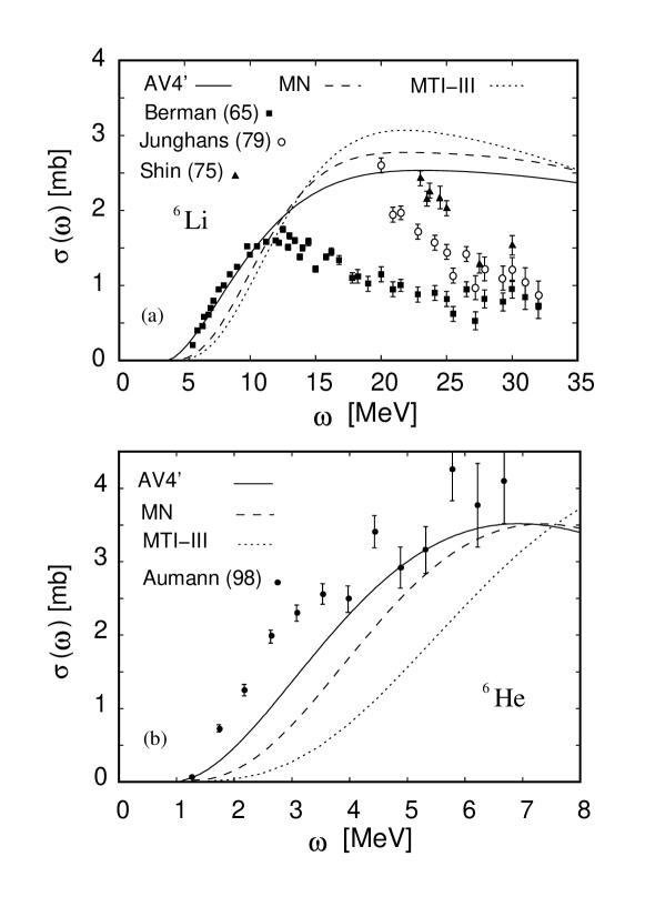
Figure 16: Theoretical and experimental photoabsorption cross section results (see also text).

Figure 17: Comparison of the theoretical photoabsorption cross section calculated with AV4’ potential with experimental data from Ahr75 .

In figure 15 the results for the total photoabsorption cross section of ⁶Li and ⁶He Li6He6a ; Li6He6b with several semirealistic potentials are shown. One notes that the general structure of the cross section is similar for the various potential models. In particular one has always the presence of two peaks in ⁶He, even if peak positions and peak heights are potential dependent, while there is one single giant dipole resonance peak in ⁶Li. The double peak structure of ⁶He can be interpreted as a response of a halo nucleus, where the low-energy peak is due to the halo–$\alpha$ core oscillation (soft dipole response) and the peak at higher energies due to the neutron-proton spheres oscillation (Gamow-Teller mode or hard dipole response). So the low-energy ⁶He peak is due to the breakup of the neutron halo. The second one, at higher $\omega$, corresponds to the breakup of the $\alpha$ core. The ⁶Li cross section does not show such a substructure. This is probably due to the fact that the breakup in two three-body nuclei, ³He + ³H, fills the gap between the halo and the $\alpha$ core peaks. Note that in case of ⁶He a corresponding breakup in two identical nuclei, ³H + ³H, is not induced by the dipole operator.

In figure 16 the theoretical results are shown together with available experimental data. For the AV4’ potential AV4' active also in P-wave, one finds an enhancement of strength in the threshold region compared to the S-wave potentials. It is evident that the inclusion of the P-wave interaction improves the agreement with experimental data considerably. This is particularly the case for ⁶Li. In fact with the AV4’ potential one has a rather good agreement with experimental data up to about 12 MeV. In case of ⁶He the increase of low-energy strength is not sufficient, there is still some discrepancy with data. Probably, in order to describe the halo structure of this nucleus in more detail additional potential parts are needed. In particular the spin-orbit component of the NN potential could play a role in the determination of the soft dipole resonance. In fact in a single particle picture of ⁶He the two halo neutrons will mainly stay in a p-state and can interact with one of the core nucleons via the NN LS-force.

Anyway the experimental situation is very confused. Again, like in the ⁴He case, no data comes from a direct measurement of the total photoabsorption cross section. Such an experiment is now in course at MaxLab in Lund for ⁶Li and we really hope that they will be able to clarify the situation.

Finally in figure 17 the total photoabsorption cross section of ⁷Li is shown. One readily notes that the gross properties of the data, steep rise, broad maximum and slow fall off, are very well reproduced quantitatively over the whole energy region by the theory. It is worthwhile to emphasize that this result is based on an ab initio calculation in which the complicated final state interaction of the 7N-system is rigorously taken into account by application of the LIT method. No adjustable parameters were used, the sole ingredient being the AV4’ NN potential model. It remains to be seen whether the slight variation of the data near and above the maximum will also be found in an experiment with improved accuracy. Such an experiment is in course at MaxLab in Lund. The new results could clarify in particular the question whether a simple semi-realistic potential like the AV4’ model is sufficient for an accurate theoretical description of this reaction or whether a more realistic nuclear force including a 3N-force is needed.

8 conclusions

In these lectures I have tried to give an overview of what one can learn from studying e.w. interactions with nuclei. The essential messages are the following.

• Since the nuclei are interacting strongly and the e.w. interaction is weak a lowest order perturbative description of the cross sections allows to focus on the nuclear dynamics.

• Understanding nuclear dynamics means understanding how the effective degrees of freedom that appear in the hamiltonian explicitly (nucleons) interact. Since these d.o.f. are not fundamental particles, but composite systems, the interaction is in principle a many-body interaction. In particular to understand the role of more than two-body forces in nuclei is an issue which is debated at present.

• An effective interaction between effective d.o.f. implies implicit d.o.f.. They constitute the bridge between nuclear physics and non perturbative QCD. Electroweak probes, differently from the hadronic ones, are sensitive to them, providing precious informations about this issue.

• In order that a comparison between theory and experiment is meaningful regarding the conclusions one can draw, it is necessary to work within theoretical ab initio approaches able to get accurate results with controlled numerical uncertainties. Due to the difficulties in solving the quantum mechanical many-body problem, especially in the continuum (many particle scattering problem), few-body systems assume an important role.

• The lorentz integral transform (LIT) method has represented a big step forward in that it has allowed to calculate ab initio e.w. cross sections with more than three nucleons in the continuum, reducing the continuum problem to a bound state problem.

• Until now applications of the LIT method, coupled with advanced bound state methods, have concentrated on systems with A=2-7. Modern realistic potentials, however, have been used up to A=4. The present challenge on the theory side is the extention to larger systems, both stable and exotic (halo).

• Confronted with the big progresses of the theory the experimental situation does not seem to have reached the same amount of accuracy, hindering in many cases the possibility to draw conclusions from the comparison theory-experiments. Therefore there is a clear necessity of experimental activity in this field, especially at lower energies and momenta.

In conclusion I hope to have been able to give an idea of the accomplishments in the field of e.w. interactions with light nuclear systems, (stable or exotic) and in particular of its future perspectives. They could be very exciting, considering the rich amount of investigations which are now made possible by the great progress in the field of few-body physics.

References

- (1) J. Bjorken and S. Drell, Relativistic Quantum Mechanics, McGraw-Hill (1964).
- (2) T. W. Donnelly and R. D. Peccei, Phys. Rept. 50, 1 (1979).
- (3) T. W. Donnelly, Prog. Part. Nucl. Phys. 13, 183 (1985).
- (4) S. Boffi, C. Giusti, F. D. Pacati, and M. Radici, Electromagnetic Response of Atomic Nuclei, Clarendon Press, Oxford, 1996.
- (5) H. Kim, S. Schramm and C. J. Horowitz, Phys. Rev. C 53, 2468 (1996).
- (6) M. B. Barbaro, A. De Pace, T. W. Donnelly, A. Molinari and M. J. Musolf, Phys. Rev. C 54, 1954 (1996).
- (7) W. M. Alberico et al., Nucl. Phys. A 623, 471 (1997).
- (8) J. D. Walecka, Electron Scattering for Nuclear and Nucleon Structure, Cambridge University Press, 2001.
- (9) H. Arenhövel and S.K. Singh, Eur. Phys. J. A 10, 183 (2001).
- (10) J.E. Amaro, M.B. Barbaro, J.A. Caballero, T.W. Donnelly, and C. Maieron, Phys. Rev. C 71, 065501(2005).
- (11) V. D. Efros, W. Leidemann, G. Orlandini, N. Barnea J. Phys. G, 34, R459 (2007).
- (12) L.L. Foldy and S.A. Wouthuysen, Phys. Rev. 78, 29 (1950).
- (13) J.M. Eisenberg and W. Greiner, Excitation mechanisms of the nucleus, Nort Holland Pub. Co., 1988, p.190.
- (14) O. Yakubovsky, Sov. J. Nucl. Phys. 5, 937 (1967).
- (15) H. Kamada and W. Glöckle, Nucl. Phys. A 548, 205 (1992).
- (16) W. Glöckle, The Quantum Mechanical Few-Body Problem, Springer-Verlag, 1983.
- (17) J. Avery, Hyperspherical Harmonics, Kluwer Academic Publishers, Dordrecht, 1989.
- (18) M. Fabre de la Ripelle, Ann. Phys. 147, 281 (1983).
- (19) M. Viviani, A. Kievsky, and S. Rosati, Few–Body Syst. 18, 25 (1995).
- (20) M. Kamimura, Phys. Rev. A 38, 621 (1988).
- (21) H. Kameyama, Kamimura, and Y. Fukushima, Phys. Rev. C 40, 974 (1989).
- (22) Y. Suzuki and K. Varga, Stochastic variational approach to quantum mechanical few-body problems, Springer-Verlag, 1998.
- (23) J. Carlson, Phys. Rev. C36, 2026 (1987).
- (24) B. S. Pudliner and V. R. Pandharipande, J. Carlson, S. C. Pieper, and R. B. Wiringa, Phys. Rev. C 56, 1720 (1997).
- (25) R. B. Wiringa, Steven C. Pieper, J. Carlson, and V. R. Pandharipande, Phys. Rev. C 62, 014001.
- (26) K. Suzuki and S.Y. Lee, Prog. Theor. Phys. 64, 2091 (1980).
- (27) P. Navrátil and B. R. Barrett, Phys. Rev. C 59, 1906 (1999).
- (28) P. Navrátil G. P. Kamuntavičius, and B. R. Barrett, Phys. Rev. C 61, 044001 (2000).
- (29) P. Navrátil, J. P. Vary, and B. R. Barrett, Phys. Rev. Lett. 84, 5728 (2000).
- (30) N. Barnea, W. Leidemann, and G. Orlandini, Phys. Rev. C 61, 054001 (2000).
- (31) N. Barnea, W. Leidemann, and G. Orlandini, Nucl. Phys. A 693, 565 (2001).
- (32) H. Kamada et al., Phys.Rev.C 64, 044001 (2001).
- (33) R.B. Wiringa, V.G.J. Stoks, and R. Schiavilla, Phys. Rev. C 51, 38 (1995).
- (34) Steven C. Pieper, R. B. Wiringa, and J. Carlson, Phys. Rev. C 70, 054325 (2004).
- (35) R. B. Wiringa, Steven C. Pieper, J. Carlson, and V. R. Pandharipande, Phys. Rev. C 62, 014001 (2000)
- (36) P. Navratil, S. Quaglioni, I. Stetcu, and B. R. Barrett, Recent developments in no-core shell-model calculations arXiv:0904.0463.
- (37) F. Coester, Nucl. Phys. 7, 421 (1958).
- (38) G. Hagen, T. Papenbrock, D. J. Dean, M. Hjorth-Jensen, and B. Velamur Asokan, Phys. Rev. C 80, 021306 (2009).
- (39) L. D. Faddeev, Sov. Phys. JETP 12, 1014 (1961).
- (40) O. Yakubowsky, Yad. Fiz. 5, 1312 (1967), Sov. J. Nucl. Phys. 5, 937 (1967).
- (41) V.D. Efros, W. Leidemann, and G. Orlandini, Phys. Lett. B 338, 130 (1994).
- (42) V.D. Efros, Yad. Fiz. 41, 1498 (1985), Sov. J. Nucl. Phys. 41, 949 (1985).
- (43) A.N. Tikhonov and V.Y Arsenin, Solutions of Ill–Posed Problems, V H Winston and Sons,(Washington, DC) 1977.
- (44) V.D. Efros, W. Leidemann, and G. Orlandini, Few–Body Syst. 14, 151 (1993).
- (45) F.S. Acton, Numerical Methods that Work, Harper & Row, New York, 1970.
- (46) E.T. Jaines, The Maximum Entropy Formalism ed R D Levune and M Tribus, Cambridge: MIT Press (1978), p.15.
- (47) D. Andreasi, W. Leidemann, Ch. Reiss, and M. Schwamb, Eur. Phys. J. A 24, 361 (2005).
- (48) C. Lanczos, J. Res. Nat. Bur. Stand. 45, 255 (1950).
- (49) G.H. Golub and C.F. Van Loan, Matrix Computations, The Johns Hopkins University Press, Baltimore, 1983.
- (50) M. A. Marchisio, N. Barnea, W. Leidemann, and G. Orlandini, Few–Body Syst. 33, 259 (2003).
- (51) E. Dagotto, Rev. Mod. Phys. 66, 763 (1994).
- (52) K.A. Hallberg, Phys. Rev. B 52, 9827 (1995).
- (53) T.D. Kühner and S.R. White, Dynamical Correlation Functions using the Density Matrix Renormalization Group ArXiv:cond–mat/9812372.
- (54) S. Martinelli, H. Kamada, G. Orlandini, and W. Glöckle, Phys. Rev. C 52, 1778 (1995).
- (55) J. Golak, R. Skibinski, W. Gloeckle, H. Kamada, A. Nogga, H. Witala, V. D. Efros, W. Leidemann, G. Orlandini, and E.L. Tomusiak, Nucl. Phys. A 707, 365 (2002).
- (56) S. Della Monaca, V.D. Efros, A. Khugaev, W. Leidemann, G. Orlandini, E. L. Tomusiak, and L. P. Yuan, Phys. Rev. C 77, 044007 (2008).
- (57) W. Leidemann, V.D. Efros, G. Orlandini, and E.L. Tomusiak, Threshold 3He and 3H Transverse Electron Scattering Response Functions, arXiv:0906.0663.
- (58) R. Machleidt, Adv. Nucl. Phys. 19, 189 (1989).
- (59) G.A. Retzlaff et al, Phys. Rev. C 49, 1263 (1994).
- (60) A. Deltuva, A.C. Fonseca, and P.U. Sauer, Phys. Lett. B 660, 471 (2008).
- (61) S. Quaglioni and P. Navratil Phys. Rev. C 79, 044606 (2009)
- (62) J.R. Calarco, B.L. Berman, and T W. Donnelly, Phys. Rev. C 27, 1866 (1983).
- (63) R.E.J Florizone et al., Phys. Rev. Lett. 72, 3476 (1994).
- (64) D.P. Wells et al., Phys. Rev. C 46, 449 (1992).
- (65) G. Ellerkmann, W. Sandhas, S. A. Sofianos, and H. Fiedeldey, Phys. Rev. C 53, 2638 (1996).
- (66) R.A. Malfliet and J. Tjon, Nucl. Phys. A 127, 161 (1969).
- (67) B.L. Berman, D.D. Faul, P. Meyer, and D.L. Olson, Phys. Rev. C 22, 2273 (1980).
- (68) V.D. Efros, W. Leidemann, and G. Orlandini, Phys. Rev. Lett. 78, 4015 (1997).
- (69) N. Barnea, V. D. Efros, W. Leidemann, and G. Orlandini, Phys. Rev. C 63, 057002 (2001).
- (70) S. Quaglioni et al., Phys. Rev. C 69, 044002 (2004).
- (71) B. Nilsson et al., Phys. Lett. B 626, 65 (2005).
- (72) T. Shima et al., Phys. Rev. C 72, 044004 (2005).
- (73) S. Nakayama et al., Phys. Rev. C 76, 021305 (2007).
- (74) S. Bacca, N. Barnea, W. Leidemann, and G. Orlandini, Phys. Rev. Lett. 102, 162501 (2009 ).
- (75) V.D. Efros, W. Leidemann, G. Orlandini, and E.L. Tomusiak, Phys. Lett. B 484, 223 (2000).
- (76) G. Feldman et al., Phys. Rev. C 42, R1167 (1990).
- (77) Yu. M. Arkatov et al., Yad. Konst. 4, 55 (1979).
- (78) A.Yu. Buki, I.S. Timchenko, N.G. Shevchenko, and I.A. Nenko, Phys. Lett. B 641, 156 (2006).
- (79) S.A. Coon and H.K. Hahn, Few-Body Syst. 30, 131 (2001).
- (80) S.A. Dytman et al., Phys. Rev. C 38, 800 (1988).
- (81) A. Zghiche et al., Nucl. Phys. A 572, 513 (1994).
- (82) J. Carlson, J. Jourdan, R. Schiavilla, and I. Sick, Phys. Rev. C 65, 024002 (2002).
- (83) V.D. Efros, W.Leidemann, G. Orlandini, and E.L. Tomusiak, Phys. Rev. C 72 011002 (2005).
- (84) D. Gazit and N. Barnea, Phys. Rev. Lett. 98, 192501 (2007).
- (85) S. Bacca, M.A. Marchisio, N. Barnea, W. Leidemann,and G. Orlandini, Phys. Rev. Lett. 89, 052502 (2002).
- (86) S. Bacca, N. Barnea, W. Leidemann,and G. Orlandini, Phys.Rev. C 69, 057001 (2004).
- (87) R.B. Wiringa and S.C. Pieper, Phys. Rev. Lett. 89 (2002) 182501.
- (88) J. Ahrens et al., Nucl. Phys. A 251, 479 (1975).