Light–like mesons and deep inelastic scattering in finite–temperature AdS/CFT with flavor

Abstract:

We use the holographic dual of a finite–temperature, strongly–coupled, gauge theory with a small number of flavors of massive fundamental quarks to study meson excitations and deep inelastic scattering (DIS) in the low–temperature phase, where the mesons are stable. We show that a high–energy flavor current with nearly light–like kinematics disappears into the plasma by resonantly producing vector mesons in highly excited states. This mechanism generates the same DIS structure functions as in the high temperature phase, where mesons are unstable and the current disappears through medium–induced parton branching. To establish this picture, we derive analytic results for the meson spectrum, which are exact in the case of light–like mesons and which corroborate and complete previous, mostly numerical, studies in the literature. We find that the meson levels are very finely spaced near the light–cone, so that the current can always decay, without a fine–tuning of its kinematics.

1 Introduction

Motivated by some experimental results at RHIC, which suggest that the deconfined matter produced in the intermediate stages of a ultrarelativistic nucleus–nucleus collision might be strongly interacting, there is currently a large interest towards understanding the properties of strongly coupled field theories at finite temperature within the framework of the AdS/CFT correspondence (see the review papers [1, 2, 3, 4, 5, 6] for details and more references). A substantial part of this effort has been concentrated on studying the response of such a plasma to energetic, ‘hard’, probes, so like heavy quarks [7, 8, 9, 10, 11, 12, 13, 14, 15, 16], mesons (or quark–antiquark pairs) [17, 18, 19, 20, 21, 22, 23, 24, 25], or photons [26, 27, 28, 29, 30, 31], in an attempt to elucidate some intriguing RHIC data, so like the unexpectedly large ‘jet quenching’, or to provide alternative signatures of a strongly–coupled matter.

In particular, AdS/CFT calculations of deep inelastic scattering (DIS) [32, 33, 26, 27, 31, 34, 35, 36, 37, 38] have given access to the structure of strongly coupled matter at high energy and for small space–time separations and thus revealed an interesting picture, which is quite different from the corresponding picture in a gauge theory at weak coupling. One has thus found that there are no point–like ‘partons’ at strong coupling, that is, no constituents carrying a sizeable fraction $x\sim\mathcal{O}{(1)}$ of the total longitudinal momentum of a ‘hadron’ [32, 33] or plasma [26, 27] at high energy. This has been interpreted as the result of a very efficient branching process through which all partons have fallen at the smallest values of $x$ which are consistent with energy conservation. This interpretation is consistent with arguments based on the operator product expansion at strong coupling [32, 39] and is further supported by the fact that the DIS structure functions were found to be large at small values of $x\ll 1$, where they admit a natural interpretation in terms of partons [33, 26, 3]. The central scale in this picture is the saturation momentum $Q_{s}(x)$, which defines the borderline between the large–$x$ and large virtuality ($Q>Q_{s}(x)$) domain which is void of partons, and the small–$x$, small virtuality ($Q\lesssim Q_{s}(x)$) domain where parton exist, with occupation numbers of order 1 (a situation somewhat reminiscent of, but more extreme than, parton saturation in QCD at weak coupling [40]). This scale $Q_{s}$ plays an essential role also for other high energy processes, of direct relevance to heavy ion collisions, like the energy loss and the momentum broadening of a heavy quark [15, 16]. It can furthermore be related to the dissociation length for a large, semiclassical, ‘meson’ [18, 19, 20, 21].

So far, most studies of DIS at finite temperature and strong coupling were concerned with the ${\mathcal{N}}=4$ supersymmetric Yang–Mills (SYM) theory, where the role of the virtual photon is played by the ${\cal R}$–current — a conserved current associated with a U(1) global symmetry which couples to massless fields in the adjoint representation of the color group SU$(N_{\rm c})$. Very recently, the same problem has been addressed [31] within the context of a ${\mathcal{N}}=2$ supersymmetric plasma obtained by adding $N_{\rm f}$ hypermultiplets of (generally massive) fundamental fields to the ${\mathcal{N}}=4$ SYM plasma, in the ‘probe’ limit where $N_{\rm f}\ll N_{\rm c}$. In that case, the ‘photon’ is a flavor current which couples to a pair of fields (fermions and scalars) in the fundamental representation of SU$(N_{\rm c})$, that we shall refer to as ‘quarks’. In order to describe the results in Ref. [31] and also our subsequent results in this paper, it is useful to briefly recall the structure of the holographic dual of the ${\mathcal{N}}=2$ plasma at strong coupling $\lambda\equiv g^{2}N_{\rm c}\gg 1$, also known as the ‘D3/D7 model’ [41, 42, 43, 4] (see also Sect. 2 below).

The supergravity fields (in particular, the Abelian gauge field dual to the flavor current) live in the worldvolume of one of the $N_{\rm f}$ D7–branes that have been inserted in the AdS${}_{5}\times S^{5}$ Schwarzschild background geometry dual to the ${\mathcal{N}}=4$ SYM plasma. For the case where the fundamental fields are massive, the D7–branes are separated in the radial direction from the $N_{\rm c}$ D3–branes located at the ‘center’ of AdS${}_{5}\times S^{5}$. The distance between the two systems of brane then fixes the ‘bare’ mass of the fundamental ‘quarks’, represented by Nambu–Goto strings stretching from a D7–brane to a D3–brane. Flavorless ‘mesons’, or quark–antiquark bound states, can be described either as strings with both endpoints on a D7–brane, or (at least for sufficiently small meson masses and spins) as normal modes of the supergravity fields propagating in the worldvolume of the D7–brane. In this paper, we shall adapt the second point of view, that of the normal modes.

For zero or sufficiently low temperatures, the mesons are strongly bound [43, 23]: their binding energy almost compensates the large quark masses (proportional to the string tension), so that the meson masses remain finite in the strong coupling limit $\lambda\to\infty$ (the ‘supergravity approximation’), to which we shall restrict ourselves. In that limit, the quarks become infinitely massive and then the mesons are stable: they form an infinite, discrete, tower of (scalar and vector) modes, distinguished by their quantum numbers. A remarkable property of the meson spectrum that will play an essential role in what follows is that, at finite temperature, the dispersion relation for a given mode changes virtuality, from time–like to space–like, with increasing momentum [23]. This is illustrated in Fig. 1. In particular, there exists an intermediate value of the momentum at which the mode becomes light–like.

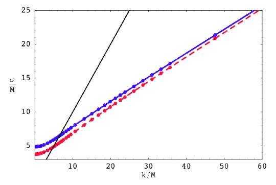
Figure 1: Dispersion relation $\omega(k)$ for the lightest spin–zero mesons in the low temperature phase, or Minkowski embedding [23]. The solid blue curve corresponds to a pseudo–scalar meson, whereas the red dashed curve corresponds to a scalar meson. The solid black line corresponds to $\omega=k$.

This situation persists for sufficiently low temperatures, so long as the D7–brane, although deformed by the attraction exerted by the black hole, remains separated from the latter. But with increasing temperature, one finds a first–order phase transition (from the ‘Minkowski embedding’ to the ‘black hole embedding’) at some critical temperature $T_{c}$, at which the tip of the D7–brane suddenly jumps into the black hole (BH) horizon [44, 23]. For $T\geq T_{c}$, all the mesons ‘melt’ : their dispersion relations acquire large imaginary parts (comparable to their real parts), showing that the bound states are now highly unstable [24, 25].

One should stress that this peculiar ‘meson melting’ phase transition is specific to this model and has no analog in QCD. The corresponding situation in QCD is not yet fully clear, but on physical grounds (given that the deconfinement ‘phase transition’ is truly a cross–over) one would expect the mesons to gradually melt when increasing $T$ above $T_{c}$, according to their sizes. The smallest mesons, those built with the heavy quarks, may survive in the temperature range pertinent to RHIC or LHC. Assuming the quark–gluon plasma to be effectively strongly coupled within this range, one could use the ‘low–temperature’ phase of this model to get some insight into the properties of the still surviving, very small and very heavy, mesons, and the ‘high–temperature’ phase for the larger, lighter, mesons that have already melt.

Returning to the problem of the DIS for the flavor current, it is quite clear that the situation is very different in the high–temperature phase ($T\geq T_{c}$) as compared to low–temperature one ($T<T_{c}$). At $T>T_{c}$, the problem is conceptually the same as for the ${\cal R}$–current in the ${\mathcal{N}}=4$ plasma [26, 27]. The space–like current fluctuates into a system of virtual partons — for the flavor current, this system involves a pair of fundamental fields together with arbitrary many ${\mathcal{N}}=4$ quanta — whose subsequent evolution depends upon the kinematics. If the energy $\omega$ of the current is low enough (for a fixed virtuality $Q$), the partonic fluctuation closes up again and essentially nothing happens: the space–like current is stable, so like in the vacuum, due to energy–momentum conservation. (We ignore here tunnel effects at finite temperature, which are exponentially small [26, 36].) But if the energy is sufficiently high, such that $\omega\gtrsim Q^{3}/T^{2}$, the virtual partons live long enough to feel the interactions with the plasma (in the dual gravity problem: the attraction exerted by the black hole) and under the influence of these interactions they keep branching until they disappear into the plasma. In the dual gravity theory, this medium–induced branching is seen as the fall of the dual gauge field into the BH horizon. Since this process is fully driven by interactions with the ${\mathcal{N}}=4$ plasma, the saturation momentum and also the DIS structure functions at small $x$ should be the same as for the ${\cal R}$–current, up to a global factor which counts the number of degrees of freedom to which couples the current ($N_{\rm c}^{2}$ for the ${\cal R}$–current and, respectively, $N_{\rm c}N_{\rm f}$ for the flavor one). This is indeed what was found in Ref. [31] for the high–temperature phase.

But at lower temperatures $T<T_{c}$, the situation turns out to be more subtle. On the supergravity side, it is a priori clear, from geometrical considerations, that the gauge field dual to the flavor current cannot fall into the black hole, for any energy: indeed, the support of this field is restricted to the worldvolume of the D7–brane, which is now separated from the BH horizon along the radial direction. This reasoning led the authors in Ref. [31] to conclude that DIS should not be possible in this case, however high is the energy. It is understood here that the high–energy limit does not commute with the large–$\lambda$ limit: the energy must remain small not only as compared to the quark mass $m_{\rm q}\sim\sqrt{\lambda}M_{\rm gap}$, but also as compared to the mass of the lowest string excitations $m_{\rm string}\sim{\lambda}^{1/4}M_{\rm gap}$ [43], which are not described by the supergravity fields. Here, $M_{\rm gap}$ is the lowest meson mass at zero temperature, and is independent of $\lambda$ (see Sect. 2 below).

Our main, new, observation is that, although it cannot fall into the BH, the flavor current can nevertheless disappear into the plasma by resonantly producing space–like vector mesons which, as already mentioned, are indeed supported by the plasma. (For a time–like current in the vacuum, the resonant production of mesons has been discussed in App. B of Ref. [25].) For this process to be possible, the kinematics of the current should match with the dispersion relations for the vector mesons. For this interaction to qualify as ‘deep inelastic scattering’, the associated structure functions — determined by the coupling of the current to the mesons and computed as the imaginary part of the current–current correlator — must be non–zero in a continuous domain of the phase–space, and not only at discrete values of the energy. In this paper, we shall demonstrate that these conditions are indeed satisfied at sufficiently high energy. Our final result is that the structure functions for flavor DIS are exactly the same in this low temperature–phase as in the high–temperature phase, although the respective physical pictures are quite different. This result is in fact natural, as we shall later explain.

To develop our arguments, we shall perform a detailed study of the meson excitations in the high–energy, space–like, kinematics relevant for DIS off a strongly coupled plasma; that is, $\omega\gg Q\gg T$, with $Q^{2}\equiv k^{2}-\omega^{2}>0$. We shall focus on vector mesons with transverse polarizations, which provide the dominant contribution to DIS at high energy [26], but we expect similar results to apply for other types of excitations (longitudinal vector mesons, scalar and pseudoscalar ones). Also, for technical reasons, we shall limit ourselves to the case of very heavy mesons, or very low temperature, $M_{\rm gap}\gg T$, which however captures all the salient features of the general situation.

Concerning the kinematics, we shall find that a space–like current can excite mesons only for high enough energies and relatively small virtualities, such that the current and the mesons are nearly light–like. This is so because a current with large space–like virtuality encounters a potential barrier near the Minkowski boundary (associated with energy–momentum conservation) and thus cannot penetrate in the inner region of the D7–brane, where mesons could be created. However, for high enough energy $\omega\gtrsim Q^{3}/T^{2}$, this barrier is overcome by the gravitational attraction due to the black hole (i.e., by the mechanical work done by the plasma [26, 27]), and then the current can penetrate inside the bulk and thus excite mesons. The corresponding kinematics being nearly light–like, $\omega\simeq k$, we shall focus our attention on the respective region of the meson dispersion relation in Fig. 1, but we shall provide analytic approximations also for the other regions (in Sect. 4). Our results are as follows.

For the strictly light–like mesons ($\omega=k$), we shall construct in Sect. 5 exact, analytic, solutions for the spectrum and the wavefunctions, which take particularly simple forms for large quantum numbers $n\gg 1$. We shall thus find an infinite tower of equally spaced levels, with high energies and a large level spacing: $\omega_{n}\simeq n\Delta\omega$ where $\Delta\omega\sim T(M_{\rm gap}/T)^{3}\gg M_{\rm gap}$. (For comparison, at zero momentum, the energy of the mode $n$ is $\omega_{n}(k=0)\sim nM_{\rm gap}$.) Similarly, for the gauge field dual to a light–like flavor current, we shall find exact ‘non–normalizable’ solutions, from which we shall compute the retarded current–current correlator in the high energy limit $\omega\gg T(M_{\rm gap}/T)^{3}$. As expected, this propagator exhibits poles at the energies of the light–like mesons, so its imaginary part is an infinite sum over delta–like resonances. The coefficient of each delta–function represents the probability for the resonant production of a meson by a current whose energy is exactly $\omega_{n}$. Conversely, they also describe the rate for the decay of a vector meson into an on–shell photon, a mechanism recently proposed as a possible signal of strong coupling behaviour in heavy ion collisions [30].

The resonant production of mesons remains possible also for slightly space–like kinematics, and, of course, for any time–like kinematics, but this is perhaps not the most interesting physical situation, as it requires the energy of the current to be finely tuned to that of a meson mode. Given the large level spacing $\Delta\omega$ indicated above, it looks at a first sight unlikely that a small uncertainty $\delta\omega\ll\omega$ in the energy of the current — as inherent in any scattering experiment (even a Gedanken one !), where the ‘photon’ is not a plane wave, but a wave packet — could help reducing the need for the fine–tuning. If that was true, it would mean that for the whole high–energy region in phase–space, except for a set of zero measure (as defined by the dispersion relations for the meson modes), the current survives in the plasma for arbitrarily long time. However, as we shall argue now, that conclusion would be a bit naive, as it underestimates the consequences of a small fluctuation in the energy, or the virtuality, of the current for the problem at hand.

The main point is that the energy uncertainty $\delta\omega$ should not be compared to the (relatively large) level spacing $\Delta\omega$ between two successive resonances, but rather to the change in energy which is necessary to cross from one meson level to another at a fixed value $k$ of the momentum. Indeed, one should not forget that the dispersion relation in the relevant kinematics is nearly light–like, that is, $\omega_{n}\simeq k_{n}$ for the $n$th mode. Hence, when increasing the energy by $\Delta\omega$ to move from one level to a neighboring one, one is simultaneously increasing the momentum $k$ by the same, large, amount — one moves along the light–cone. But in a scattering problem, the momentum $k$ of the current is fixed and its energy $\omega$ has generally an uncertainty $\delta\omega$, related to the fact that the source producing the current has been acting over a finite period of time $\delta t$: $\delta\omega\sim 1/\delta t$. Before we discuss this time $\delta t$, let us make the crucial observation that the meson levels are very finely spaced in energy when probed at a fixed value of $k$. This is a general feature of the high–energy kinematics, which is further amplified by the peculiar shape of the meson dispersion relation near the light–cone.

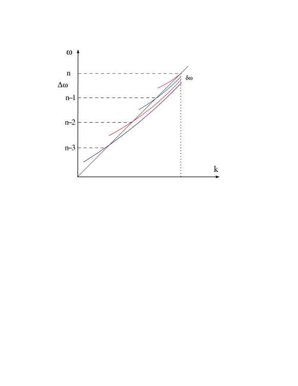
Figure 2: Qualitative illustration of the meson dispersion relation $\omega(k)$ in the vicinity of the light–cone. Four successive modes are shown. Although widely spaced along the light–cone, the modes are close to each other at any given value of $k$. Thus, in order to jump from one mode to a neighboring one, one needs a relatively large energy jump $\Delta\omega$ at fixed virtuality $Q$, but only a small energy jump $\delta\omega$ at fixed momentum $k$.

As a simpler example, recall first the situation at zero temperature [43], where the meson dispersion relation reads, schematically, $\omega_{n}(k)=(k^{2}+n^{2}M_{\rm gap}^{2})^{1/2}\simeq k+n^{2}M_{\rm gap}^{2}/2k$, with the approximate equality holding when $k\gg nM_{\rm gap}$. Hence the energy jump $\delta\omega_{n}(k)\equiv\omega_{n+1}(k)-\omega_{n}(k)$ needed to cross from one mode to another at fixed $k$ is $\delta\omega_{n}(k)\simeq nM_{\rm gap}^{2}/k$ and becomes smaller and smaller when increasing $k$. As anticipated, the modes are very finely spaced at large $k$. Returning to the finite–$T$ case of interest, it turns out that the respective dispersion relation is even more sensitive to small variations in the virtuality of the mode near the light–cone. Specifically, we shall find in Sects. 4.3 and 6 that the level spacing at fixed $k$ defined as above scales with $k$ as $\delta\omega_{n}(k)\sim T(T/k)^{1/3}$ when $k\simeq k_{n}=n\Delta\omega$ (see Fig. 2). As anticipated, this is considerably smaller than the energy spacing $\Delta\omega\sim T(M_{\rm gap}/T)^{3}$ at fixed virtuality : indeed, $\Delta\omega/\delta\omega_{n}\sim n^{1/3}(M_{\rm gap}/T)^{4}\gg 1$.

To understand the typical energy uncertainty $\delta\omega$ of the current, one needs an estimate for its interaction time in the plasma $t_{\rm int}$. Indeed, the source producing the current should act over a comparatively shorter time $\delta t\lesssim t_{\rm int}$ in order for the subsequent dynamics to be observable. Via a time–dependent analysis of the dynamics of the dual gauge field in Sect. 6, we shall find that $t_{\rm int}$ is controlled by the progression of the gauge field within the D7–brane, which yields $t_{\rm int}\sim(k/T)^{1/3}/T$ (similarly to the ${\cal R}$–current [27]). This estimate implies a lower limit $\delta\omega\gtrsim 1/t_{\rm int}$ on the energy uncertainty of the current which is of the order of the level spacing $\delta\omega_{n}$ indicated above. This justifies performing an average over neighboring levels in the calculation of the imaginary part of the current–current correlator. This averaging smears out the meson resonances and produces our main result in this paper, Eq. (5.18). As anticipated, this result is identical to the DIS structure functions in the high–temperature phase, which shows that the current is completely absorbed by the plasma in both cases.

The analysis in Sect. 6 also allows us to deduce a space–time picture for the nearly light–like mesons in the semiclassical regime at large quantum numbers $n\gg 1$, where the notion of a classical orbit makes sense. We thus find that the period for one orbit is $\Delta t_{n}\sim(\omega_{n}/T)^{1/3}/T$, where we recall that the energy of the bound state is $\omega_{n}=n\Delta\omega$. Furthermore, we find that the meson spends the major part of this time far away from the tip of the D7–brane, at relatively large radial distances $\sim\omega_{n}^{1/3}$. This is so because its orbital velocity is much higher near the tip than at larger radial distances. It is finally interesting to notice that, in this light–like kinematics, the period $\Delta t_{n}$ of the bound state has the same parametric dependence upon its energy as the interaction time $t_{\rm int}$ of the current, and similarly for the typical radial location of the meson versus the saturation momentum $Q_{s}(k)\sim k^{1/3}$ for the current.

2 Mesons in the D3/D7 brane model at finite temperature

According to the AdS/CFT correspondance [47, 48, 49], the four–dimensional ${\cal N}=4$ super–Yang–Mills (SYM) gauge theory with ‘color’ gauge group SU$(N_{\rm c})$ is dual to a type IIB string theory living in the ten–dimensional curved space–time AdS${}_{5}\times S^{5}$, which describes the decoupling limit of $N_{\rm c}$ black D3–branes. By further adding a black brane to this geometry, one obtains the holographic dual of the finite–temperature, plasma, phase of the ${\cal N}=4$ SYM [50]. The ensuing metric reads (see, e.g., [1])

$${\rm d}s^{2}=\frac{u^{2}}{L^{2}}\left(-f(u){\rm d}t^{2}+{\rm d}{\bm{x}}^{2}\right)+\frac{L^{2}}{u^{2}}\left(\frac{{\rm d}u^{2}}{f(u)}+u^{2}{\rm d}\Omega_{5}^{2}\right)\,,$$ (2.1)

where $f(u)=1-u_{0}^{4}/u^{4}$, with $u_{0}=\pi L^{2}T$ the radial position of the black hole horizon and $T$ the common temperature of the ${\cal N}=4$ SYM plasma and of the black hole. The curvature radius $L$ is defined in terms of the string coupling constant $g_{s}$ and the string length scale $\ell_{s}$ via $L^{4}=4\pi g_{s}N_{\rm c}\,\ell_{s}^{4}$. The holographic dictionary relates the gauge and string theory coupling constants as $g^{2}=4\pi g_{s}$. In the “strong coupling limit” of the gauge theory, defined as $N_{\rm c}\rightarrow\infty$, $\lambda\equiv g^{2}N_{\rm c}\rightarrow\infty$, with $g$ fixed and small ($g\ll 1$), the string theory reduces to classical supergravity theory in the AdS${}_{5}\times S^{5}$ Schwarzschild geometry with metric (2.1).

All fields in the ${\cal N}=4$ SYM theory transform in the adjoint representation of SU$(N_{\rm c})$. Fields transforming in the fundamental representation of the gauge group can be introduced in the gravity dual by inserting a second set of D–branes in the supergravity background [41, 4]. In particular, we consider the decoupling limit of the intersection of $N_{\rm c}$ black D3–branes and $N_{\rm f}$ D7–branes as described by the array:

$$\begin{array}[]{ccccccccccc}&0&1&2&3&4&5&6&7&8&9\\ {\rm D3}&\times&\times&\times&\times&&&&&&\\ {\rm D7}&\times&\times&\times&\times&\times&\times&\times&\times&&\\ \end{array}$$ (2.2)

where the first four dimensions (0, 1, 2, and 3) correspond to the Minkowski coordinates $\{t,x^{i}\}$ and the last six ones (from 5 to 9) to the six–dimensional space with coordinates $\{u,\Omega_{5}\}$. The dual field theory is now an ${\cal N}=2$ gauge theory consisting of the original SYM theory coupled to $N_{\rm f}$ fundamental hypermultiplets which consists of two Weyl fermions and their superpartner, complex, scalars (see e.g. [51]). For brevity, we shall globally refer to these fundamental fields as ‘quarks’. In the limit where the number of flavors is relatively small, $N_{\rm f}\ll N_{\rm c}$, the D7–branes may be treated as probes in the black D3–brane geometry (2.1). That is, the D7–branes are generally deformed by their gravitational interactions with the D3–branes and the black hole, but one can neglect their back reaction on the ambient geometry, Eq. (2.1). The ensuing geometry is dual to a ${\cal N}=2$ plasma at finite temperature in which the effects of the fundamental degrees of freedom (say, on thermodynamical quantities) represent only small corrections, of relative order $g^{2}N_{\rm f}=\lambda(N_{\rm f}/N_{\rm c})\ll 1$ (see e.g. [23]).

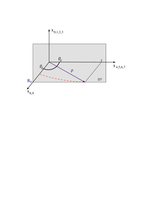
Figure 3: Schematic representation of the geometry of the D3–D7 model at finite temperature. This drawing is adapted to the low–temperature, or very heavy quark, situation, where $R_{0}\gg\rho_{0}=1$. See the text for more explanations.

Although both the D3–branes and the D7 ones fill the Minkowski space, these two types of branes need not overlap with each other, as they can be separated in the 89–directions, which are orthogonal to both of them. When this happens, the conformal symmetry is explicitly broken already at classical level and then the fundamental fields in the dual gauge theory become massive: their ‘bare’ mass is proportional to the radial separation $u_{m}$ between the two sets of branes at zero temperature. Indeed, a fundamental field is ‘dual’ to an open string connecting a D7–brane to a D3–brane, so its ‘bare’ mass is equal to the string length $u_{m}$ times the string tension:

$$m_{\rm q}\,=\,\frac{u_{m}}{2\pi\ell_{s}^{2}}\,=\,\sqrt{\lambda}\,\frac{u_{m}}{2\pi L^{2}}\,.$$ (2.3)

To render such geometrical considerations more suggestive, it is helpful to perform some changes of coordinates [44, 23]. First, we introduce a new, dimensionless, radial coordinate $\rho$, related to the coordinate $u$ via

$$(u_{0}\rho)^{2}=u^{2}+\sqrt{u^{4}-u_{0}^{4}}\,.$$ (2.4)

Note that that the BH horizon corresponds to $\rho_{0}=1$ and the Minkowski boundary to $\rho\to\infty$, with $u_{0}\rho\simeq\sqrt{2}u$ when $u\gg u_{0}$ (i.e., $\rho\gg 1$). Then the background metric (2.1) becomes

$${\rm d}s^{2}=\frac{1}{2}\left(\frac{u_{0}\rho}{L}\right)^{2}\left[-{f^{2}\over\tilde{f}}\,{\rm d}t^{2}+\tilde{f}{\rm d}{\bm{x}}^{2}\right]+\frac{L^{2}}{\rho^{2}}\left[{\rm d}\rho^{2}+\rho^{2}{\rm d}\Omega_{5}^{2}\right]\,,$$ (2.5)

where

$$f(\rho)=1-\frac{1}{\rho^{4}}\,,\,\,\,\,\,\tilde{f}(\rho)=1+\frac{1}{\rho^{4}}\,.$$ (2.6)

It is furthermore useful to adapt the metric on the five–sphere to the D7–brane embedding. Since the D7–brane spans the 4567-directions, we introduce spherical coordinates $\{r,\Omega_{3}\}$ in this space and $\{R,\phi\}$ in the orthogonal 89–directions. Denoting by $\theta$ the angle between these two spaces, we have (see also Fig. 3)

$$\rho^{2}=r^{2}+R^{2}\,,\,\,\,\,\,r=\rho\cos\theta\,,\,\,\,\,\,R=\rho\sin\theta\,,$$ (2.7)

and therefore

$${\rm d}\rho^{2}+\rho^{2}{\rm d}\Omega^{2}_{5} = {\rm d}\rho^{2}+\rho^{2}\left({\rm d}\theta^{2}+\cos^{2}\theta\,{\rm d}\Omega^{2}_{3}+\sin^{2}\theta\,{\rm d}\phi^{2}\right)\,$$ (2.8)

$$= {\rm d}r^{2}+r^{2}{\rm d}\Omega^{2}_{3}+{\rm d}R^{2}+R^{2}{\rm d}\phi^{2}\,.$$

Note that, on the D7–brane, the Minkowski boundary lies at $r\to\infty$.

To specify the D7–brane (background) embedding, we require translational symmetry in the 0123–space and rotational symmetry in the 4567–directions, and fix $\phi=0$. Then the embedding can be described as the profile function $R=R_{v}(r)$. The subscript ‘$v$’ on $R_{v}$ stays for the ‘meson vacuum’: the small fluctuations of the D7–brane around its stationary geometry are dual to low–lying ‘mesons’ in the boundary gauge theory, i.e., (colorless and flavorless) bound states which involve a pair of fields from a fundamental hypermultiplet — say, a quark–antiquark pair. Such mesons are represented by strings with both ends on the D7–branes and thus can be studied (at least for small enough meson sizes and masses; see below) by examining the small fluctuations of the worldvolume fields on the D7–branes. These include the fluctuations $\delta\phi$ and $\delta R$ in the shape of the D7–brane — which give rise to pseudo–scalar and scalar mesons, respectively —, and also fluctuations of the worldvolume gauge fields, which describe vector mesons. The ‘vacuum’ profile function $R_{v}(r)$ and the spectrum of the various type of fluctuations have been systematically studied in the literature, via analytic methods in the zero–temperature case [43], and via mostly numerical methods at non–zero temperature [42, 44, 23, 24, 25]. In what follows, we shall collect the previous results which are relevant for the present analysis, with a minimum of formulæ.

The dynamics of the D7–brane is described the Dirac–Born–Infeld (DBI) action. The profile function $R_{v}(r)$ for the ‘vacuum’ embedding is obtained by solving the equation of motion for $R(r)$ which follows from this action. The meson spectrum is then obtained by solving the linearized equations of motion (EOM) which follow after expanding the DBI action to quadratic order in small fluctuations around the ‘vacuum’ embedding.

At zero temperature, one finds that the ‘vacuum’ profile is trivial, i.e., independent of $r$ :

$$R_{v}(r)\,=\,R_{0}\,=\,\sqrt{2}\,\frac{u_{m}}{u_{0}}\qquad\mbox{ (zero temperature)}\,,$$ (2.9)

where we recall that $u_{m}$ is the separation between the two types of brane in the original radial coordinate $u$. (At $T=0$, Eq. (2.4) reduces to $\rho\equiv\sqrt{2}(u/u_{0})$ where $u_{0}$ is an arbitrary reference scale, which drops out from the final results.) The EOM for the small fluctuations have been solved exactly, in terms of hypergeometric functions [43]. At zero temperature, both Lorentz symmetry and supersymmetry are manifest. Accordingly, for a meson with four–momentum $q^{\mu}=(\omega,0,0,k)$, the dispersion relation $\omega(k)$ involves only the ‘invariant mass’ combination $M^{2}\equiv\omega^{2}-k^{2}$. Besides, this relation depends upon two ‘quantum numbers’: a ‘radial’ number $n=0,1,2,...$, which counts the number of zeroes of the corresponding wavefunction in the interval $0<r<\infty$, and an ‘angular’ number $\ell$, with $\ell=0,1,2,...$, which refers to rotations along the $S^{3}$ component of the D7–brane. (In the dual gauge theory, $\ell$ represents a charge under the internal symmetry group SO(4) which is dual to rotations on $S^{3}$.) Supersymmetry together with the global SO(4) symmetry imply additional degeneracies for the meson spectrum, as discussed in [43]. Specifically, Ref. [43] found the following dispersion relation

$$M^{2}(n,\ell)\,\equiv\,\omega_{n\ell}^{2}(k)-k^{2}\,=\,\frac{u_{m}^{2}}{L^{4}}\,4(n+\ell+1)(n+\ell+2)$$ (2.10)

for both (pseudo)scalar and vector mesons. Note the presence of a mass gap in the spectrum: the mass of the lightest mesons is non–zero, namely,

$$M_{\rm gap}\,=\,2\sqrt{2}\,\frac{u_{m}}{L^{2}}\,.$$ (2.11)

Note also that the meson masses are much smaller, by a factor $1/\sqrt{\lambda}$, than the bare quark mass, Eq. (2.3). This shows that in this strong coupling limit the mesons are tightly bound: in the total energy, the binding energy almost cancels the mass of the quarks.

At finite temperature, the D7–brane feels the attraction exerted by the black hole and thus is deflected towards the latter — the stronger the deviation, the shorter is the radial separation $u$ (or $\rho$) between the two. This deflection becomes negligible towards the Minkowski boundary ($r\to\infty$), where the profile function $R_{v}(r)$ approaches the value $R_{0}$ that it would have (at any $r$) at $T=0$. More precisely, for asymptotically large $r$ one finds [42, 44, 23]

$$R_{v}(r)\,\simeq\,R_{0}\,-\,\frac{c}{r^{2}}\,,$$ (2.12)

with $R_{0}$ related to the ‘bare’ quark mass, as in Eq. (2.3), and $c$ a positive number proportional to the quark condensate.

On the other hand, closer to the black hole horizon ($\rho\sim 1$), one finds two different types of behaviour — corresponding to two thermodynamically distinct phases separated by a first–order phase transition —, depending upon the ratio $M_{\rm gap}/T=2\pi R_{0}$ between the (zero–$T$) mass gap and the temperature: (i) for relatively large values of $R_{0}$, larger than a critical value numerically found as $R_{c}\simeq 1.306$ [23], the D7–branes close off above the black hole horizon (‘low–temperature’, or ‘Minkowski embeddings’); (ii) for $R_{0}<R_{c}$, the D7–branes extend through the horizon (‘high–temperature’, or ‘black hole embeddings’). In the gauge theory, the most striking feature of this transition is the change in the meson spectrum [44] : in the low temperature phase, the spectrum of mesons has a mass gap and the bound states are stable, so like at $T=0$ [23]; in the high temperature phase, there is no mass gap and the mesonic excitations are unstable and characterized by a discrete spectrum of quasinormal modes (i.e., they have dispersion relations with non–zero, and large, imaginary parts) [24, 25].

For the reasons explained in the Introduction, in this paper we shall restrict ourselves to the low–temperature phase, in which the mesons are stable. The corresponding dispersion relations have been numerically computed in Ref. [23], at least within restricted regions of the phase space. As expected, the spectrum shows deviations from both Lorentz symmetry and supersymmetry, and these deviations become more and more important with increasing temperature (for a given $M_{\rm gap}$). What was perhaps less expected and, in any case, remarkable is the pattern of the violation of the Lorentz symmetry by the spectrum: when increasing the momentum $k$ of a given mode (i.e., , for fixed values of $n$ and $\ell$, which remain good ‘quantum numbers’ also at finite temperature), the ‘virtuality’ $-Q^{2}\equiv\omega_{n\ell}^{2}(k)-k^{2}$ of that mode is continuously decreasing, from time–like values ($-Q^{2}>0$) at relatively low $k$ to space–like values ($-Q^{2}<0$) for sufficiently large $k$, in such a way that, for asymptotically large $k$, the dispersion relation approaches a limiting velocity which is strictly smaller than one:

$$\omega(k)\,\simeq\,v_{0}\,k\,\quad\mbox{with \ $v_{0}\,<\,1$ \ as \ $k\,\to\,\infty$}\,.$$ (2.13)

It has been furthermore noticed in the numerical analysis in Ref. [23] that, with increasing $k$, the mode wavefunction becomes more and more peaked near the bottom ($r\to 0$) of the D7–brane. This led to the interesting suggestion, which was furthermore confirmed by the numerical results, that the limiting velocity $v_{0}$ coincides with the local velocity of light at $r\approx 0$, i.e., $\rho\approx R_{v}(0)$ :

$$v_{0}\,\simeq\,\left.\sqrt{-\frac{g_{tt}}{g_{zz}}}\right|_{r=0}=\frac{f(R_{v}(0))}{\tilde{f}(R_{v}(0))}\,.$$ (2.14)

As we shall later argue in Sect. 4, this identification follows indeed from the respective EOM. Our analytic study will also clarify other aspects of the dispersion relation, like the precise conditions for the onset of the asymptotic behaviour (2.13) and the subleading corrections to it, which in particular contain the dependence upon the quantum numbers $n$ and $\ell$. More generally, we shall be able to construct piecewise analytic approximations for the dispersion relation $\omega_{n\ell}(k)$ and also for the wavefunctions of the modes, which will confirm the numerical findings in Ref. [23] and provide further, analytic, insight into these results. Although, in our analysis, we shall cover all kinematical domains in $k$ and thus provide a global picture for the meson spectrum, our main focus will be on the nearly light–light mesons with $\omega\simeq k$. Indeed, as we shall explain in the next section, this regime is the only one to be relevant for the deep inelastic scattering of the flavor current.

3 Deep inelastic scattering off the ${\cal N}=2$ plasma

The ${\cal N}=2$ theory with $N_{\rm f}$ flavors of equal mass has a global $U(N_{\rm f})\simeq SU(N_{\rm f})\times U(1)_{\rm q}$ symmetry (describing flavor rotations of the fields in the fundamental hypermultiplets), to which one can associate $N_{f}^{2}$ conserved currents bilinear in the ‘quark’ operators (see Appendix A in [25] for explicit expressions). In particular, the current $J^{\mu}_{\rm q}$ corresponding to the diagonal subgroup $U(1)_{\rm q}$ is associated with the conservation of the net ‘quark’ number (i.e., the number of fundamental quarks and scalars minus the number of antiquarks and hermitean conjugate scalars). By adding to the theory a U(1)_e.m. gauge field $A_{\mu}$ minimally coupled to this $J^{\mu}_{\rm q}$ current (with an ‘electromagnetic’ coupling which is arbitrarily small), one can construct a model for the electromagnetic interactions and thus set up a Gedanken deep inelastic scattering experiment which measures the distribution of the fundamental fields inside the plasma. One can visualise this process as the exchange of a virtual, space–like, ‘photon’ (as described by the field $A_{\mu}$) between the strongly coupled ${\cal N}=2$ plasma at finite temperature and a hard lepton propagating through the plasma.

3.1 Equations of motion in the D3/D7 brane model

Within the D3/D7 brane model, the flavor current $J^{\mu}_{\rm q}$ is dual to an abelian gauge field $A_{m}$ living in the worldvolume of the D7–brane, whose dynamics is encoded in the DBI action. According to the gauge/gravity duality, the correlation functions of the operator $J^{\mu}_{\rm q}$ are obtained from the ‘non–renormalizable’ modes of the field $A_{m}$, that is, the solutions to the classical EOM in the bulk of the D7–brane which obey non–trivial (Dirichlet) boundary conditions at the Minkowski boundary: as $r\to\infty$, the solution $A_{m}$ must approach the U(1)_e.m. gauge field $A_{\mu}$ which acts as a source for the current $J^{\mu}_{\rm q}$. This should be contrasted to the ‘normalizable’ modes dual to vector mesons, which must vanish sufficiently fast when approaching the Minkowski boundary (see below for details).

In particular, the DIS cross–sections (or ‘structure functions’) are obtained from the (retarded) current–current correlator

$$\Pi^{\mu\nu}(q)\,\equiv\,i\int{\rm d}^{4}y\,{\rm e}^{-iq\cdot y}\,\theta(y_{0})\,\langle[J^{\mu}_{\rm q}(y),J^{\nu}_{\rm q}(0)]\rangle_{T}\,,$$ (3.1)

where the brackets $\langle\cdots\rangle_{T}$ denote the thermal expectation value in the ${\cal N}=2$ plasma. To compute this two–point function, it is enough to study the linearized EOM for the bulk field $A_{m}$, i.e., the same equations which determine the spectrum of the low–lying vector mesons, but with different boundary conditions at $r\to\infty$.

Specifically, the polarization tensor (3.1) can be given the following tensorial decomposition (in a generic frame) :

$$\Pi_{\mu\nu}(q,T)=\left(\eta_{\mu\nu}-\frac{q_{\mu}q_{\nu}}{Q^{2}}\right)\Pi_{1}(x,Q^{2})+\left(n_{\mu}-q_{\mu}\frac{n\cdot q}{Q^{2}}\right)\left(n_{\nu}-q_{\nu}\frac{n\cdot q}{Q^{2}}\right)\Pi_{2}(x,Q^{2})\,,$$ (3.2)

where $\Pi_{1}$ and $\Pi_{2}$ are scalar functions, $n^{\mu}$ is the four–velocity of the plasma in the considered frame, $Q^{2}=q_{\mu}q^{\mu}>0$ is the (space–like) virtuality of the current, and

$${x}\,\equiv\,\frac{Q^{2}}{-2(q\cdot n)T}$$ (3.3)

is the Bjorken variable for DIS off the plasma. Via the optical theorem, the DIS structure functions are obtained as

$$F_{1}(x,Q^{2})\,=\,\frac{1}{2\pi}\,{\rm Im}\,\Pi_{1},\qquad F_{2}(x,Q^{2})\,=\,\frac{-(n\cdot q)}{2\pi T}\,{\rm Im}\,\Pi_{2}\,.$$ (3.4)

In what follows, it will be convenient to compute the (boost–invariant) structure functions by working in the plasma rest frame, where $n^{\mu}=(1,0,0,0)$ and $q^{\mu}=(\omega,0,0,k)$, and therefore $Q^{2}=k^{2}-\omega^{2}$ and $x={Q^{2}}/{2\omega T}$. However, one should keep in mind that the physical interpretation of the results is most transparent in the plasma ‘infinite momentum frame’, i.e., a frame in which the plasma is boosted at a large Lorentz factor $\gamma\gg 1$. Then, the kinematic invariants $Q^{2}$ and $x$ specify the transverse area ($\sim 1/Q^{2}$) and, respectively, the longitudinal momentum fraction (equal to $x$) of the plasma constituent (‘parton’) which has absorbed the space–like ‘photon’, and the structure functions represent parton distributions.

The piece of the DBI action which is quadratic in the gauge fields reads (see e.g. [25])

$$S_{8}=-\frac{(2\pi\ell_{s}^{2})^{2}}{4}T_{\rm D7}N_{\rm f}\int{\rm d}^{8}\sigma\sqrt{-g}\,g^{mp}g^{nq}F_{mn}F_{pq}\,,$$ (3.5)

where $T_{\rm D7}=2\pi/(2\pi\ell_{s})^{8}g_{s}$, the space–time indices $m,n,p,q$ run over the eight directions in the worldvolume of the D7–brane, $g_{mn}$ is the induced metric on the D7–brane, and $F_{mn}=\partial_{m}A_{n}-\partial_{n}A_{m}$. As already mentioned, the EOM must be solved with the following boundary conditions

$$A_{m}(t,\bm{x},r\to\infty)\,\to\,A_{\mu}(t,\bm{x})\,=\,A_{\mu}^{(0)}\,{\rm e}^{-i\omega t+ikz}\,,$$ (3.6)

which together with the fact that the equations are linear and homogeneous in all the worldvolume directions but $r$ imply that the solution $A_{m}$ is such that $A_{r}=A_{S^{3}}=0$ (i.e., the radial and $S^{3}$–components of the gauge field are identically zero) and the remaining, four, components $A_{\mu}(t,\bm{x},r)$, with $\mu=t,x,y,z$, are plane–wave in the Minkowski directions with $r$–dependent coefficients. Since the gauge fields are independent of the coordinates on $S^{3}$, one can reduce Eq. (3.5) to an effective action in the relevant five dimensions. The induced metric in these directions, that we denote as $\tilde{g}_{mn}$, follows from Eqs. (2.5)–(2.8) as

$${\rm d}s^{2}(\tilde{g})=\frac{1}{2}\left(\frac{u_{0}\rho}{L}\right)^{2}\left[-{f^{2}\over\tilde{f}}\,{\rm d}t^{2}+\tilde{f}{\rm d}{\bm{x}}^{2}\right]+\frac{L^{2}}{\rho^{2}_{v}}\left(1+\dot{R}_{v}^{2}\right){\rm d}r^{2}\,,$$ (3.7)

where $\rho^{2}_{v}=r^{2}+R^{2}_{v}(r)$, $\dot{R}_{v}={\rm d}R_{v}/{\rm d}r$, and we recall that $R_{v}(r)$ is the profile of the D7–brane embedding. After integrating over the coordinates on $S^{3}$, the action (3.5) reduces to

$$S=-\frac{(2\pi\ell_{s}^{2})^{2}}{4}\Omega_{3}T_{\rm D7}N_{\rm f}\int{\rm d}t{\rm d}^{3}x{\rm d}r\,\frac{\sqrt{-\tilde{g}}}{g_{\rm eff}^{2}(r)}\,\tilde{g}^{mp}\tilde{g}^{nq}F_{mn}F_{pq}\,,$$ (3.8)

where $\Omega_{3}=2\pi^{2}$, $m,n,\dots=t,x,y,z,r$, and

$$\frac{1}{g_{\rm eff}^{2}(r)}\equiv\left(\frac{Lr}{\rho_{v}}\right)^{3}\ \ \Longrightarrow\ \ \frac{\sqrt{-\tilde{g}}}{g_{\rm eff}^{2}(r)}\,=\,\frac{u_{0}^{4}}{4}\,r^{2}f\tilde{f}\sqrt{1+\dot{R}_{v}^{2}}\,.$$ (3.9)

Clearly, the EOM generated by the action (3.7) read

$$\partial_{m}\left(\frac{\sqrt{-\tilde{g}}}{g_{\rm eff}^{2}(r)}\,\tilde{g}^{mp}\tilde{g}^{nq}F_{pq}\right)\,=\,0\,.$$ (3.10)

The propagation of the virtual photon along the $z$ axis introduces an anisotropy axis in the problem, so the equations of motion look different for the longitudinal ($\mu=t,z$) and respectively transverse ($\mu=x,y$) components of the gauge field. In what follows we shall focus on the transverse fields, $A_{i}$ with $i=x,y$, since from the experience with the ${\cal R}$–current [26, 27] we expect these fields to provide the dominant contributions to the structure functions $F_{1,2}$ in the high energy limit. Moreover, our final argument in Sect. 5 will allow us to also reconstruct the flavor longitudinal structure function $F_{L}=F_{2}-2xF_{1}$ from the corresponding one for the ${\cal R}$–current. The relevant components of the field strength tensor are $F_{ri}=\partial_{r}A_{i}$, $F_{ti}=\partial_{t}A_{i}\to-i\omega A_{i}$, and $F_{zi}=\partial_{z}A_{i}\to ikA_{i}$, and the equation satisfied by $A_{i}(r)$ reads

$$\ddot{A}_{i}+\left[\partial_{r}\ln\left(\frac{\sqrt{-\tilde{g}}}{g_{\rm eff}}\,\tilde{g}^{rr}\tilde{g}^{ii}\right)\right]\dot{A}_{i}\,+\,\frac{\tilde{g}^{zz}}{\tilde{g}^{rr}}\left(\frac{\tilde{f}^{2}}{f^{2}}\,\omega^{2}-k^{2}\right)A_{i}\,=\,0.$$ (3.11)

This equation must be solved with the Dirichelet boundary condition (3.6) at $r\to\infty$ together with the condition of regularity at $r=0$. The solution to this boundary–value problem is a ‘non–normalizable’ mode, as opposed to the ‘normalizable’ modes which describe vector meson excitations of the D7–brane: the latter are the solutions Eq. (3.11) which vanish sufficiently fast (namely, like $A_{i}(r)\sim 1/r^{2}$) when $r\to\infty$ [43, 23].

Once the ‘non–normalizable’ solution is known as a (linear) function of the boundary value $A_{i}^{(0)}$, the current–current correlator (3.1) is obtained, roughly speaking, by taking the second derivative of the classical action (i.e., the action (3.8) evaluated with that particular solution) with respect to $A_{i}^{(0)}$. This procedure is unambiguous in so far as the euclidean (i.e., imaginary–time) correlators are concerned, but it misses the imaginary part for the real–time correlators. Rather, the correct prescription for computing the retarded polarization tensor (3.1) reads (for the case of $\Pi_{xx}=\Pi_{yy}=\Pi_{1}$) [53, 54]

$$\Pi_{1}(x,Q^{2})\,=\,-\frac{N_{\rm f}N_{\rm c}T^{2}}{8}\,\left[r^{3}\,\frac{\partial_{r}A_{i}(r,\omega,k)}{A_{i}(r,\omega,k)}\right]_{r\to\infty}\,,$$ (3.12)

where $i$ is either $x$ or $y$. The overall normalization factor reflects the fact that the flavor current couples to $N_{\rm c}N_{\rm f}$ fundamental fields. When using the above formula, the precise normalization at $r\to\infty$, i.e., the boundary value $A_{i}^{(0)}$, becomes irrelevant, as it cancels in the ratio. Note that, in order to make use of Eq. (3.12), it is enough to know the solution in the vicinity of the the Minkowski boundary. But to that aim, one generally needs to solve the EOM for arbitrary values of $r$, since the second boundary condition is imposed at $r=0$.

In general, the coefficients in Eq. (3.11) are rather complicated functions, as visible on Eqs. (3.7) and (3.9), and this complication hinders the search for analytic solutions. However, how we now explain, they can be considerably simplified without loosing any salient feature by restricting ourselves to the very low temperature, or very heavy meson, case $R_{0}\gg 1$, or $M_{\rm gap}\gg T$. This restriction entails two important types of simplifications. The first one refers to the ‘vacuum’ profile $R_{v}(r)$, which in the general case is known only numerically [23], but which becomes essentially flat when $R_{0}\gg 1$. Indeed, in that case, the maximal deviation from the asymptotic value $R_{0}$, namely (see App. A in Ref. [23]),

$$R_{v}(0)-R_{0}\,\simeq\,-\,\frac{1}{2R_{0}^{7}}\,\ll\,1\,,$$ (3.13)

is truly negligible, so one can use $R_{v}(r)\simeq R_{0}$ (and hence $\dot{R}_{v}=0$) at any $r$.

The second type of simplifications refer to the BH horizon at $\rho_{0}=1$ : when $R_{0}\gg 1$, the condition $\rho\gg 1$ is automatically satisfied at any point within the worldvolume of the D7–brane. Then, the thermal effects encoded in $f$ and $\tilde{f}$, which scale like $1/\rho^{4}$, cf. Eq. (2.6), can be safely neglected in all the terms in Eq. (3.11) except for the last one: indeed, within that term, the finite–$T$ deviations $1-f$ and $1-\tilde{f}$ are potentially amplified by the large energy factor $\omega$. Specifically (with $\rho^{2}=R_{0}^{2}+r^{2}$)

$$\frac{\tilde{f}^{2}}{f^{2}}\,\omega^{2}-k^{2}\,=\,(\omega^{2}-k^{2})\,+\,\frac{4/\rho^{4}}{1-2/\rho^{4}}\,\omega^{2}\,\simeq\,-Q^{2}\,+\,\frac{4}{\rho^{4}}\,\omega^{2}\,,$$ (3.14)

where we have also used $Q^{2}=k^{2}-\omega^{2}$.

To summarize, under the assumption that $R_{0}\gg 1$, the EOM for the transverse gauge fields $A_{i}(r)$ takes a particularly simple form:

$$\ddot{A}_{i}+\frac{3}{r}\,\dot{A}_{i}\,+\left(-\frac{2{\bar{Q}}^{2}}{\rho^{4}}\,+\,\frac{8\bar{\omega}^{2}}{\rho^{8}}\right)A_{i}\,=\,0\,,$$ (3.15)

where $\dot{A}_{i}={\rm d}A_{i}/{\rm d}r$, $\rho^{2}=R_{0}^{2}+r^{2}$, and we have introduced the dimensionless variables

$$\bar{\omega}\,\equiv\,\omega\,\frac{L^{2}}{u_{0}}\,=\,\frac{\omega}{\pi T}\,,\qquad\bar{k}\,\equiv\,k\,\frac{L^{2}}{u_{0}}\,=\,\frac{k}{\pi T}\,,\qquad\bar{Q}^{2}\,\equiv\,\bar{k}^{2}-\bar{\omega}^{2}\,.$$ (3.16)

One should emphasize here that this condition $R_{0}\gg 1$ introduces no loss of generality, neither for a study of the DIS process (in which case we are anyway interested in $\omega,\,\bar{Q}\gg T$, and then the dominant dynamics takes place at large radial distances $\rho\gg 1$ [26, 27]), nor for that of the meson spectrum (for which we shall find results which are consistent with the numerical analysis in Ref. [23], although that analysis was performed for $R_{0}\sim\mathcal{O}{(1)}$).

Although considerably simpler than the original equation (3.11), the above equation is still too complicated to be solved exactly, except in the special case $\bar{Q}=0$, to be discussed in Sect. 5. For more general situations, related to either the meson spectrum or the problem of DIS, we shall later construct analytic approximations. In preparation for that and in order to gain more insight into the role of the various terms in Eq. (3.15), it is useful to first consider a different but related problem, whose solution is already known : this is the DIS of the ${\cal R}$–current [32, 33, 26, 27].

3.2 Some lessons from the ${\cal R}$–current

The ${\cal R}$–current is a conserved current associated with one of the U(1) subgroups of a global SU(4) symmetry of the ${\cal N}=4$ SYM theory. The respective operator is bilinear in the massless, adjoint, fields of ${\cal N}=4$, and remains conserved even in the presence of the fundamental hypermultiplets (i.e., in ${\cal N}=2$ theory), because of the probe limit $g^{2}N_{\rm f}\ll 1$. The supergravity field dual to the ${\cal R}$–current is, once again, a gauge field $A_{\mu}$, whose dynamics however is not anymore restricted to the worldvolume of the D7–brane — rather, this field can propagate everywhere in the AdS${}_{5}\times S^{5}$ Schwarzschild space–time, in particular, it can fall into the black hole. Because of that, the D7–brane plays no role in the case of the ${\cal R}$–current, so the following discussion applies to both ${\cal N}=4$ and ${\cal N}=2$ theories (with $N_{\rm f}\ll N_{\rm c}$, of course).

For a space–like ${\cal R}$–current with high virtuality $Q\gg T$ and for large radial coordinates $\rho\gg\rho_{0}$, the dynamics of the dual ${\cal R}$–field $A_{i}(r)$ is described by an equation similar to Eq. (3.15), but where the variables $\rho$ and $r$ are now identified with each other (since $R_{0}$ plays no role in this case). That is,

$$\ddot{A}_{i}+\frac{3}{\rho}\,\dot{A}_{i}\,+\left(-\frac{2{\bar{Q}}^{2}}{\rho^{4}}\,+\,\frac{8\bar{\omega}^{2}}{\rho^{8}}\right)A_{i}\,=\,0\qquad\mbox{(${\cal R}$--current)}\,,$$ (3.17)

where now $\dot{A}_{i}={\rm d}A_{i}/{\rm d}\rho$ and it is understood that $\rho\gg 1$.

The dynamics is driven by the competition between the two terms inside the brackets in Eq. (3.17). The first term, proportional to $Q^{2}$, acts as a potential barrier which opposes to the progression of the field towards the interior of AdS₅ : by itself, this would confine the field near the Minkowski boundary, at large radial distances $\rho\gtrsim\rho_{Q}\equiv\bar{Q}$. The second term, proportional to $\omega^{2}$, is present only at finite temperature (as manifest from its derivation in Eq. (3.14)) and it represents the gravitational attraction between the gauge field and the BH. For sufficiently small values of $\rho$, smaller than $\rho_{c}\equiv({2\bar{\omega}/\bar{Q}})^{1/2}$, this attraction overcomes the repulsive barrier $\propto Q^{2}$, and then the overall potential becomes attractive. However, unless the energy $\bar{\omega}$ is high enough, this change in the potential has no dynamical consequences, because the field is anyway stuck near the Minkowski boundary and thus cannot feel the attraction. Clearly a change in the dynamics will occur when the energy is so high that $\rho_{c}\gtrsim\rho_{Q}$, which requires $\bar{\omega}\gtrsim\bar{Q}^{3}$, or, in physical units, $\omega\gtrsim Q^{3}/T^{2}$. When this happens, the potential barrier at $\rho\to\infty$ cannot prevent the gauge field to penetrate (through diffusion; see the discussion in Sect. 6) down to the attractive part of the potential at $\rho\lesssim\rho_{c}$, and from that point on, the potential barrier plays no role anymore. Hence, the dynamics at radial distances $1\ll\rho\lesssim\rho_{c}$ is controlled by the even simpler equation

$$\ddot{A}_{i}+\frac{3}{\rho}\,\dot{A}_{i}\,+\,\frac{8\bar{\omega}^{2}}{\rho^{8}}\,A_{i}\,=\,0\qquad\mbox{(${\cal R}$--current \& high energy)}\,,$$ (3.18)

which does not involve $\bar{Q}$ and thus is formally the same as the equation describing a light–light current. This equation can be exactly solved in terms of Airy functions. The general solution reads (up to an overall normalization, which is irrelevant)

$$A_{i}(\rho)\,=\,c{\rm Ai}(-\xi)\,+\,{\rm Bi}(-\xi)\,,\qquad\xi\,\equiv\,\left(\frac{\sqrt{2}\bar{\omega}}{\rho^{3}}\right)^{2/3}\,,$$ (3.19)

valid for $(\bar{Q}/\bar{\omega}^{1/3})\lesssim\xi\ll\bar{\omega}^{2/3}$. This involves one unknown coefficient $c$ which can be fixed, in principle, by matching onto the corresponding solution at smaller distances $\rho\sim\mathcal{O}{(1)}$, which in particular obeys the appropriate boundary condition at $\rho=\rho_{0}=1$. This boundary condition is rather clear on physical grounds: the gauge field can be only absorbed by the BH, but not also reflected, hence the near–horizon solution must be a infalling wave [53, 2], i.e., a field which with increasing time approaches the horizon.

The solution near $\rho=1$ obeying this boundary condition can be explicitly computed, and its matching onto Eq. (3.19) can indeed be done [26], but it turns out that this actually not needed for the purpose of computing the DIS structure function: the problem of the ${\cal R}$–current offers an important simplification, which is worth emphasizing here, since the same simplification appears for the flavor current in the high–temperature case (the ‘black hole embedding’) [31], but not also in the low–temperature, or ‘Minkowski’, embedding of interest for us here. Namely, the infalling boundary condition can be enforced not only near the BH horizon, but also at much larger values of $\rho$, where Eq. (3.19) applies. This is so since there is no qualitative change in the shape of the potential at any intermediate point in the range $1<\rho\ll\rho_{c}$ which could give rise to a reflected wave.

The last observation allows us to identify $c=i$ in Eq. (3.19): indeed, consider this approximate solution for $\rho\ll\bar{\omega}^{1/3}$, or $\xi\gg 1$, where one can resort on the asymptotic expansions for the Airy functions. Using Eq. (3.19) with $c=i$, one obtains

$$A_{i}(t,z,\rho)\,\simeq\,\frac{1}{\sqrt{\pi}\xi^{1/4}}\,\exp\left\{-i\omega t+ikz+i\frac{2}{3}\,\xi^{3/2}+i\frac{\pi}{4}\right\}\quad\mbox{for}\quad 1\,\ll\,\rho\,\ll\,\bar{\omega}^{1/3}\,,$$ (3.20)

which is indeed an infalling wave.

Now that the coefficient $c$ has been fixed, one can use the approximate solution (3.19) for relatively small values of $\xi$ and compute the current–current correlator according to Eq. (3.12). (One can adapt Eq. (3.12) to the ${\cal R}$–current by multiplying its r.h.s by a factor $N_{\rm c}/4N_{\rm f}$.) Specifically, Eq. (3.19) is still correct for $\xi\sim\bar{Q}/\bar{\omega}^{1/3}\ll 1$, where one can use the small–$\xi$ expansions for the Airy functions, and thus deduce [26]

$$F_{1}\,=\,\frac{3N_{\rm c}^{2}T^{2}}{16\Gamma^{2}(1/3)}\left(\frac{\bar{\omega}}{6}\right)^{{2}/{3}}\,,\qquad F_{2}\,\sim\,{x}F_{1}\,\sim\,xN_{\rm c}^{2}Q^{2}\left(\frac{T}{xQ}\right)^{{2}/{3}}\,,$$ (3.21)

where in the last estimate we indicated the parametric dependencies of the structure functions upon the variables relevant for DIS. As it should be clear from the previous discussion, these results hold for sufficiently high energy, $\omega\gtrsim{Q^{3}}/{T^{2}}$, a condition which can be rewritten in terms of the DIS variables $x$ and $Q^{2}$ as

$$x\,\equiv\,\frac{Q^{2}}{2\omega T}\ \lesssim\ x_{s}(Q)\,\equiv\,\frac{T}{Q}\,,\qquad\mbox{or}\qquad Q\ \lesssim\ Q_{s}(x)\,\equiv\,\frac{T}{x}\,.$$ (3.22)

On the other hand, for larger values of Bjorken–$x$, $x\gg T/Q$, or higher virtualities $Q\gg Q_{s}$, the structure functions are exponentially small (since generated through tunelling). This strong suppression of the structure functions at large values of $x$ and/or $Q^{2}$ implies the absence of point–like constituents in the strongly coupled plasma [32, 33, 26, 27]. The critical value $Q_{s}(x)\sim T/x$ is known as the saturation momentum, since Eq. (3.21) is consistent with a parton picture in which partons occupy the phase space at $Q\lesssim Q_{s}(x)$ with occupation numbers of $\mathcal{O}{(1)}$ [26].

Returning to the flavor current of interest here, let us now identify the similarities and the differences with respect to the problem of the ${\cal R}$–current, that we have just discussed.

In the high–temperature case, where the tip of the D7–brane enters the BH horizon, there are no serious conceptual differences with respect to the ${\cal R}$–current. For $r\gg 1$, Eq. (3.15) is still valid, so the large–$r$ dynamics is exactly the same as discussed in relation with Eq. (3.19). At smaller $r\sim\mathcal{O}{(1)}$, the EOM becomes more complicated (in particular because of the $r$–dependence of the profile function $R_{v}(r)$, which is non–trivial in that high–temperature case), but there is no ingredient in the dynamics which could prevent the fall of the flavor field $A_{i}$ into the BH. Hence, the appropriate boundary condition at $\rho=1$ (the tip of the D7–brane) is still the infalling one, and moreover this condition can again be enforced ar large $r\gg 1$, where Eq. (3.19) applies. As before, this condition fixes $c=i$, thus finally yielding the same result for the DIS structure function as in Eq. (3.21), except for the overall normalization:

$$F_{1}\,\simeq\,\frac{3N_{\rm c}N_{\rm f}T^{2}}{4\Gamma^{2}(1/3)}\left(\frac{\bar{\omega}}{6}\right)^{{2}/{3}}\qquad\mbox{(flavor current in the BH embedding)}\,.$$ (3.23)

This is indeed the result found in [31]. In particular, the saturation momentum for the flavor current (in this high–temperature regime, at least) is exactly the same as for the ${\cal R}$–current, cf. Eq. (3.22), since fully determined by the current interactions with the BH.

Consider now the low–temperature phase, which is the most interesting case for us here. For the DIS problem, it is natural to assume that $Q\gtrsim M_{\rm gap}\gg T$, or $\bar{Q}\gtrsim R_{0}\gg 1$. The situation near the Minkowski boundary will be quite similar to that for the ${\cal R}$–current: At relatively low energies $\bar{\omega}\ll\bar{Q}^{3}$, there is a potential barrier at $\rho\gtrsim\bar{Q}>R_{0}$, which however disappears at larger energies $\bar{\omega}\gtrsim\bar{Q}^{3}$. When this happens, the flavor field can penetrate all the way within the worldvolume of the D7–brane. However, this worldvolume ends up at $\rho=R_{0}\gg\rho_{0}$, so there is clearly no possibility for this field to fall into the BH. Accordingly, the infalling boundary conditions do not apply here, but rather must be replaced by the condition of regularity at $\rho=R_{0}$ (the tip of the D7–brane). In order to establish the fate of the high–energy current, we therefore cannot make the economy of actually solving Eq. (3.15) for all the values of $\rho$ down to $R_{0}$. Still, there is an important ‘technical’ simplification which occurs at high energy: then, the potential barrier $\propto\bar{Q}^{2}$ plays no role anymore, so it is sufficient to consider the $\bar{Q}=0$ version of Eq. (3.15). This equation also determines the spectrum of the light–like mesons in the plasma and, as we shall see, these two problems — the flavor DIS and the light–like mesons — are indeed strongly related to each other.

4 Meson spectrum at low temperature

In this section we shall construct piecewise approximations to the spectrum of the meson excitations in the low temperature phase, or Minkowski embedding, with the purpose of clarifying some global properties of the spectrum numerically obtained in Ref. [23] and exhibited in Fig. 1. In particular, we shall follow the transition of the dispersion relation of a given mode from time–like to space–like with increasing momentum $k$, and thus identify the ‘critical’ momentum $k_{n}$ at which the mode with radial quantum number $n$ crosses the light–cone. Also we shall recover previous analytic results in the literature which concentrated on special limits, like zero–temperature [43] or very high momentum [22]. The particular case of a light–like mode ($\omega_{n}(k)=k$) will be given further attention in the next section, where we shall construct the exact respective solutions for both normalizable and non–normalizable modes, with the purposes of understanding DIS.

4.1 Equation of motion in Schrödinger form

For the subsequent analysis, it is convenient to change the definition of the radial coordinate once again, in such a way that the infinite interval $0\leq r<\infty$ be mapped into the compact interval $0\leq\zeta\leq 1$. Here $\zeta$ is defined as

$$\zeta\,\equiv\,\frac{r^{2}}{\rho^{2}(r)}\,=\,\frac{r^{2}}{R_{0}^{2}+r^{2}}\,,$$ (4.1)

so in particular the Minkowski boundary corresponds to $\zeta=1$. Then Eq. (3.15) becomes

$$\left(\partial_{\zeta}^{2}\,+\,\frac{2}{\zeta}\partial_{\zeta}\,-\,\frac{\kappa^{2}}{4\zeta(1-\zeta)}\,+\,\frac{4\Omega^{2}(1-\zeta)}{\zeta}\right)\Phi(\zeta)\,=\,0\,,$$ (4.2)

where we have replaced the name of the function by $\Phi$, for more generality: indeed, Eqs. (3.15) or (4.2) apply not only to transverse vector mesons, but also to the pseudoscalar mesons corresponding to small fluctuations in the azimuthal angle $\phi$ (the angle in the 89–plane transverse to the D7–brane; recall that the ‘vacuum’ embedding corresponds to $\phi=0$). Furthermore, we have defined

$$\kappa^{2}\,\equiv\,\frac{2\bar{Q}^{2}}{R_{0}^{2}}\,,\qquad\Omega^{2}\,\equiv\,\frac{\bar{\omega}^{2}}{2R_{0}^{6}}\,,$$ (4.3)

where the virtuality $\bar{Q}^{2}=\bar{k}^{2}-\bar{\omega}^{2}$ can now take any sign (and thus the same is true for $\kappa^{2}$). It is furthermore convenient to rewrite Eq. (4.2) in the form of a Schrödinger equation, i.e., to remove the term involving the first derivative; this can be done by writing

$$\Phi(\zeta)\,=\,\frac{1}{\zeta}\,\psi(\zeta)\,.$$ (4.4)

The corresponding “Schrödinger equation” reads

$$\left(-\partial_{\zeta}^{2}\,+\,V_{\ell}(\zeta)\right)\psi(\zeta) \,=\, 0\,,$$ (4.5)

$$V_{\ell}(\zeta)\,\equiv\,\frac{\ell(\ell+2)}{[2\zeta(1-\zeta)]^{2}} \,+\, \frac{\kappa^{2}}{4\zeta(1-\zeta)}\,-\,\frac{4\Omega^{2}(1-\zeta)}{\zeta}\,,$$ (4.6)

where we have allowed for one further generalization by adding to the potential the term corresponding to a generic value $\ell$, with $\ell=0,1,2,\dots$, for the angular ‘quantum number’ corresponding to rotations around the $S^{3}$–sphere internal to the D7–brane. (Such rotations cannot be excited by either the flavor or the ${\cal R}$–current considered in the previous section, so $\ell=0$ in the case of DIS. But modes with non–zero $\ell$ can be excited by other operators in the boundary gauge theory, which are charged under the global SO(4) symmetry of the fundamental hypermultiplets [43, 23, 25].) Since the radial coordinate $\zeta$ terminates at $\zeta=1$, it is understood that the potential becomes an infinite wall at that point; given the structure of Eq. (4.6), this additional constraint has no consequence except in the limiting case where $\ell=0$ and $\kappa^{2}=0$. The zero temperature case is obtained by formally taking $\Omega=0$ in Eq. (4.6).

Since we are interested in the normalizable modes describing mesons, we shall look for solutions $\psi_{\ell}(\zeta)$ to Eq. (4.5) obeying the following boundary conditions [43] :

$$\psi_{\ell}(\zeta)\,\propto\,\begin{cases}\displaystyle{\zeta^{\frac{\ell+2}{2}}}&\text{ for\, $\zeta\,\to\,0$}\\[5.69046pt] \displaystyle{(1-\zeta)^{\frac{\ell+2}{2}}}&\text{ for\, $\zeta\,\to\,1$}.\end{cases}$$ (4.7)

In what follows we would like to follow the change in the dispersion relation when increasing the meson momentum $k$ for fixed quantum numbers (i.e., for a given mode). This study will drive us through different regimes in terms of the variables $\kappa^{2}$ and $\Omega^{2}$. The potential $V(\zeta)\equiv V_{\ell=0}(\zeta)$ in these various regimes is illustrated in Figs. 4 and 5.

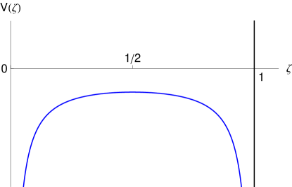
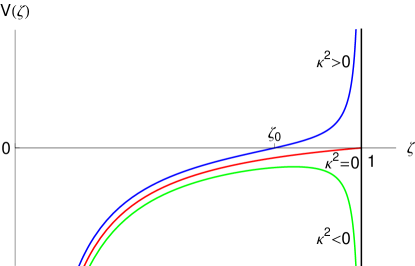
Figure 4: The potential $V(\zeta)$ in Eq. (4.6) for $\ell=0$. Left: the case where $\Omega\ll\kappa$ (as relevant at zero temperature, or for finite temperature but relatively small momenta $\bar{k}\ll nR_{0}^{3}$). Right: the case where $|\kappa|\ll\Omega$ (this corresponds to modes with momenta $\bar{k}\sim nR_{0}^{3}$).

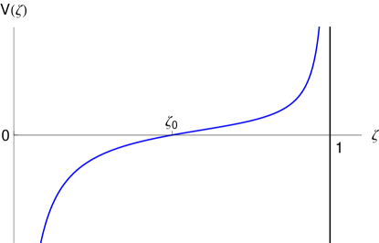
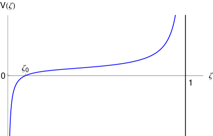
Figure 5: The potential $V(\zeta)$ in Eq. (4.6) for $\ell=0$ and relatively large, space–like, virtualities, with $\kappa<4\Omega$. Left: $\kappa=2\Omega$. Right: $\kappa\simeq 4\Omega$ (the limiting velocity regime).

4.2 The low momentum regime: time–like dispersion relation

When the momentum $k$ is sufficiently small (see Eq. (4.10) below for the precise condition), the dispersion relation is time–like ($\kappa^{2}<0$) and it is such that the last term, proportional to $\Omega^{2}$, in the potential becomes negligible (so that the potential has the symmetric shape shown in Fig. 4 left). Then Eq. (4.2) is formally the same as at zero temperature and the corresponding solutions are known exactly [43]. Namely, the solution obeying the right boundary condition at $\zeta=0$, cf. Eq. (4.7), reads (the overall normalization is chosen for convenience)

$$\psi_{\ell}(\zeta) \,=\, [\zeta(1-\zeta)]^{\frac{\ell+2}{2}}\,F(a,b;\ell+2;\zeta)\,,$$ (4.8)

$$\mbox{with}\quad a \,\equiv\, \frac{1}{2}\big{(}2\ell+3+\sqrt{1+\mu^{2}}\big{)}\,,\quad b\,\equiv\,\frac{1}{2}\big{(}2\ell+3-\sqrt{1+\mu^{2}}\big{)}\,,$$

where $F(a,b;c;x)$ is the usual hypergeometric function, also denoted as ${}_{2}F_{1}(a,b;c;x)$, which obeys $F(a,b;c;0)=1$ (see e.g. Chapter 15 in [55]) and we have set $-\kappa^{2}\equiv\mu^{2}>0$. For Eq. (4.8) to also obey the correct boundary condition at $\zeta=1$, the hypergeometric function must be regular at that point, which for the indicated values of the parameters $a,b$ and $c=\ell+2$ requires the hypergeometric series to terminate [55]. That is, $b=-n$ with $n=0,1,2,...$, and then $F(a,-n;c;x)$ is a polynomial of degree $n$ in $\zeta$. This condition yields the vacuum–like (i.e., $T=0$) spectrum in Eq. (2.10), that is,

$$\mu^{2}(n,\ell)\,\equiv\,\frac{2(\bar{\omega}_{n\ell}^{2}(k)-\bar{k}^{2})}{R_{0}^{2}}\,=\,4(n+\ell+1)(n+\ell+2)\,.$$ (4.9)

At finite temperature, Eq. (4.9) remains a good approximation so long as one can neglect the term $\propto\Omega^{2}$ in the potential, that is, for $\Omega^{2}_{n}\ll\mu^{2}_{n}$ or, equivalently (recall (4.3)), $\bar{\omega}\ll nR_{0}^{3}$. Since we also assume $R_{0}\gg 1$, it is clear that this condition is satisfied up to relatively high values of the momentum $k$, namely so long as

$$\bar{k}\,\ll\,nR_{0}^{3}\,,\qquad\mbox{or}\qquad k\,\ll\,n\,(M_{\rm gap}^{3}/T^{2})\,.$$ (4.10)

Note that we include the radial quantum number within parametric estimates, e.g., $\mu_{n}\sim n$ or $\bar{\omega}_{n}\sim nR_{0}$, since we shall be also interested in large values $n\gg 1$ (whereas $\ell$ will never be too large). Although, for definiteness, we refer to the kinematical domain (4.10) as the ‘low–momentum regime’, it is clear that, towards the upper end of this domain, the momenta are so large that $k\gg M_{n}\sim nM_{\rm gap}$ and thus the dispersion relation becomes nearly light–like.

Still within this low–momentum regime, it is easy to see that the main effect of the “finite–$T$” term $\propto\Omega^{2}$ in the potential (4.6) is to decrease the meson virtuality as compared to its “zero–$T$” value (4.9). Indeed, a simple estimate for this effect is obtained by replacing $\mu^{2}\to\mu^{2}+16\Omega^{2}$ in the l.h.s. of Eq. (4.9) (this procedure overestimates the correction when $\zeta\simeq 1$, but it should be correct at least qualitatively); hence the corrected virtuality reads

$$\mu^{2}(k,n,\ell)\,\approx\,\mu^{2}_{(0)}(n,\ell)\,-\,16\Omega^{2}_{n\ell}\,,\quad\mbox{with}\quad\mu^{2}_{(0)}(n,\ell)\,\equiv\,4(n+\ell+1)(n+\ell+2)\,.$$ (4.11)

In particular, for non–relativistic momenta ($k\ll M_{n}\sim nM_{\rm gap}$), the above dispersion relation can be expanded out as (the quantum numbers are kept implicit)

$$\omega(k)\,\approx\,M_{\rm rest}\,+\,\frac{k^{2}}{2M_{\rm kin}}\,,\quad\mbox{with}\quad M_{\rm rest}\approx M_{(0)}(1-2/R^{4}_{0})\,,\quad M_{\rm kin}\approx\frac{M_{(0)}}{1-2/R^{4}_{0}}\ ,$$ (4.12)

and therefore $M_{\rm rest}M_{\rm kin}\approx M_{(0)}^{2}$. ($M_{(0)}$ denotes the “zero–$T$” meson mass, as given by Eq. (2.10) or (4.9).) The estimates (4.12) are in fact in agreement with the respective numerical findings in Ref. [23] (see the discussion of Eq. (4.45) there).

4.3 The intermediate momentum regime: light–like dispersion relation

With further increasing $k$, the energy $\omega_{n}$ of the mode $n$ is also increasing and the last term, proportional to $\Omega^{2}$, in the potential (4.6) becomes more and more important. Since, at the same time, the virtuality $\mu_{n}^{2}$ of the mode is decreasing, it should be clear that for sufficiently large $k$ — namely, when $\bar{k}\sim nR_{0}^{3}$ — one enters a regime where $\Omega^{2}_{n}\gg\mu_{n}^{2}$ and then the roles of the respective terms in the potential are interchanged: the term in $\Omega^{2}$ becomes the dominant one, while that in $\mu^{2}$ represents only a small correction. Then the mode $n$ is nearly light–like and in fact it crosses the light cone (i.e., its virtuality $\mu_{n}^{2}(k)$ changes sign) when varying $k$ within this domain. We have not been able to analytically follow this transition, but the fact that it actually happens is quite obvious by inspection of the shape in the potential in this regime. This is shown in Fig. 4 right for the three cases of interest: (a) $\kappa^{2}\equiv-\mu^{2}$ is negative but small, (b) $\kappa^{2}=0$, and (c) $\kappa^{2}$ is positive but small.

Namely, consider the genuine Schrödinger equation associated to this potential, that is,

$$\left(-\partial_{\zeta}^{2}\,+\,V(\zeta)\right)\psi(\zeta)\,=\,E\psi(\zeta)\,,$$ (4.13)

where $E$ is the energy of a bound state. Given the shape of the potential in Fig. 4 right, it is clear that bound states with both positive and negative energies will exist for all the three cases aforementioned. It is furthermore clear that, with increasing $\Omega^{2}$ at fixed $\kappa^{2}$ the potential becomes more and more attractive, so some of the bound states will cross from positive to negative energies. This means that, for any fixed value of $\kappa^{2}$, there exist corresponding values of $\Omega^{2}$ such that the respective bound states have $E=0$. These are, of course, the meson modes that we are interested in.

This Schrödinger argument also suggest the use of the semi–classical WKB method for computing the meson spectrum. Given the shape of the potential this should be a reasonable approximation at least for sufficiently large numbers $n\gg 1$ (we set $\ell=0$ for simplicity). The Bohr–Sommerfeld quantization condition for the mode $n$ with energy $E_{n}=0$ reads

$$n\pi\,=\,\int_{0}^{\zeta_{0}}{\rm d}\zeta\,\sqrt{-V(\zeta)}\,,$$ (4.14)

where $\zeta_{0}$ is the turning point in the potential, that is, $\zeta_{0}=1$ when $\kappa^{2}\leq 0$ and $\zeta_{0}=1-\kappa/4\Omega$ when $\kappa^{2}>0$. When $\kappa=0$, the integral is straightforward and yields

$$\Omega_{n}\,\approx\,n\,,\qquad\mbox{or}\qquad\bar{\omega}_{n}\,\approx\,\sqrt{2}\,n\,R_{0}^{3}\,.$$ (4.15)

That is, the mode $n$ crosses the light–cone at $k=k_{n}$ with $\bar{k}_{n}\approx\sqrt{2}nR_{0}^{3}$. As we shall see in Sect. 5, this is indeed the correct result when $n\gg 1$.

An interesting property of the spectrum near the light–cone, which will play an important role in our subsequent study of DIS (see Sect. 5) and can be also understood on the basis of Eq. (4.14), is the extreme sensitivity of the dispersion relation to changes in the virtuality $\kappa^{2}$ around $\kappa=0$ : so long as $|\kappa^{2}|\ll\Omega^{2}$, a small change in $\kappa^{2}$ entails a large change in $\Omega^{2}$. Before we explain the origin of this property, let us first use Eq. (4.14) to render it more specific. Consider the space–like case $\kappa^{2}>0$ for definiteness, and denote $\varepsilon\equiv\kappa/4\Omega\ll 1$, so that the turning point lies at $\zeta_{0}=1-\varepsilon$. Changing the integration variable according to $x\equiv 1-\zeta$, we can successively write

$$\frac{n\pi}{2\Omega} \,=\, \int_{\varepsilon}^{1}{\rm d}x\sqrt{\frac{x^{2}-\varepsilon^{2}}{x(1-x)}}\,\simeq\,\frac{\pi}{2}+\int_{0}^{1}\frac{{\rm d}x}{\sqrt{x(1-x)}}\left(\Theta(x-\varepsilon)\sqrt{x^{2}-\varepsilon^{2}}-x\right)$$

$$\,\simeq\, \frac{\pi}{2}\,-\,\varepsilon^{3/2}\int_{0}^{\infty}\frac{{\rm d}\lambda}{\sqrt{\lambda}}\left(\lambda-\Theta(\lambda-1)\sqrt{\lambda^{2}-1}\right),$$

where we have observed that, after subtracting the dominant contribution $\pi/2$ to the first integral, the subtracted integral is dominated by its lower limit $x=\varepsilon$; this allowed us to perform the simplifications in the second line, where we denoted $x\equiv\lambda\varepsilon$. The final integral multiplying $\varepsilon^{3/2}$ is clearly a positive number of $\mathcal{O}{(1)}$. One can combine together the space–like and time–like cases into the following formula

$$n\approx\Omega_{n}\,-\,{\rm sgn}(\kappa^{2})C\sqrt{\frac{|\kappa|^{3}}{\Omega_{n}}}\qquad\mbox{for}\qquad|\kappa|\,\ll\,\Omega\,,$$ (4.17)

where $C$ is a positive constant and ${\rm sgn}(x)=\Theta(x)-\Theta(-x)$ is the sign function. This formula shows that, when moving away from the light–cone, say, towards space–like virtualities, the energy of the mode grows by a substantial amount $\Delta\Omega_{n}\sim 1$ for a relatively modest increase in the virtuality, from $\kappa=0$ to $\kappa\sim\Omega_{n}^{1/3}\ll\Omega_{n}$. In physical units, we change $\bar{\omega}_{n}$ by a large amount $\Delta\bar{\omega}_{n}\sim R_{0}^{3}\gg 1$ when increasing $\bar{Q}$ from zero to $\bar{Q}\sim n^{1/3}R_{0}\sim\bar{\omega}_{n}^{1/3}$.

This strong sensitivity of the dispersion relation to $\kappa^{2}$ around $\kappa=0$ can be traced back to the behavior of the potential near the turning point $\zeta_{0}$ (recall that it is this turning point which controls the $\kappa$–dependence of the integral in Eq. (4.14)). Namely, from Eq. (4.6) we deduce (for positive $\kappa$ with $\kappa\ll\Omega$)

$$\frac{\partial V}{\partial\kappa^{2}}\Bigg{|}_{\zeta=\zeta_{0}}\,\simeq\,\frac{\Omega}{\kappa}\,\gg\,1\,,\quad\mbox{and}\quad\frac{\partial(-V)}{\partial\Omega^{2}}\Bigg{|}_{\zeta=\zeta_{0}}\,\simeq\,\frac{\kappa}{\Omega}\,\ll\,1\,.$$ (4.18)

4.4 The high momentum regime: space–like dispersion relation

Consider now further increasing the momentum $\bar{k}$ of the mode $n$, beyond the critical value $\bar{k}_{n}\approx\sqrt{2}nR_{0}^{3}$ at which the dispersion relation crosses the light–cone. Then the virtuality of the mode $\bar{Q}_{n}$ will increase as well, i.e., the mode becomes more and more space–like (although, as we shall see, this virtuality remains relatively small, in the sense that $\bar{\omega}_{n}\simeq\bar{k}\gg\bar{Q}_{n}$). For instance, Eq. (4.17) implies that, so long as $\kappa\ll\Omega$, the virtuality grows with the energy (or the momentum) according to

$$\kappa_{n}\,\sim\,\Omega_{n}\left(\frac{\Omega_{n}-n}{\Omega_{n}}\right)^{2/3}\,,\qquad\mbox{or}\qquad\bar{Q}_{n}\,\sim\,\frac{\bar{k}^{1/3}}{R_{0}^{2}}\,\Big{(}\bar{k}-\bar{k}_{n}\Big{)}^{2/3}\,.$$ (4.19)

Eventually, when $\Omega_{n}\gg n$, $\kappa_{n}$ becomes comparable with $\Omega_{n}$ and then the potential (4.6) has the shape shown in Fig. 5 (for $\ell=0$ and two different values of $\kappa$).

As manifest on these pictures, when increasing the ratio $\kappa/\Omega$, the turning point $\zeta_{0}=1-\kappa/4\Omega$ in the potential moves towards $\zeta=0$, i.e., towards the bottom of the D7–brane. Thus, clearly, the attractive region of the potential, which can support Schrödinger bound states with energy $E_{n}=0$ (or, equivalently, space–like mesons), exists only so long as $\kappa\leq 4\Omega$, and becomes very tiny ($\zeta_{0}\ll 1$) when $\kappa$ approaches the upper limit $4\Omega$ (cf. Fig. 5 right). What we would like to argue in what follows is that for sufficiently large momentum $\bar{k}\gg nR_{0}^{3}$, the dispersion relation approaches this kinematical limit in which $\kappa_{n}\simeq 4\Omega_{n}$: this is the ‘limiting velocity’ regime, previously mentioned in relation with Eq. (2.14) [23, 22].

To that aim, let us compute the spectrum in the regime where $\kappa$ is indeed close to, but smaller than $4\Omega$, in such a way that $\zeta_{0}\ll 1$. The corresponding modes will be localized in the classically permitted region at $\zeta\leq\zeta_{0}$. It is then a good approximation to replace the potential (4.6) by its expansion near $\zeta=0$. The ensuing Schrödinger–like equation reads

$$\left(-\partial_{\zeta}^{2}\,+\,\frac{\ell(\ell+2)}{4\zeta^{2}}\,-\,\frac{2e^{2}}{\zeta}\,+\,2{\cal E}\right)\psi_{l}(\zeta)\,=\,0\,,$$ (4.20)

where we have denoted

$$2e^{2} \,\equiv\, 4\Omega^{2}\,-\,\frac{\kappa^{2}}{4}\,\simeq\,8\Omega\left(\Omega-\frac{\kappa}{4}\right)\,,$$

$$2{\cal E} \,\equiv\, 4\Omega^{2}\,+\,\frac{\kappa^{2}}{4}\,\simeq\,8\Omega^{2}\,.$$ (4.21)

When deriving Eq. (4.20) and also when simplifying the expressions in Eq. (4.4) we have anticipated the fact that, for the mode $n$, both $\Omega$ and $\kappa$ are very large but relatively close to each other, such that

$$\Omega_{n}\,,\,\kappa_{n}\,\gg\,n\,,\qquad\Omega_{n}\,-\,\frac{\kappa_{n}}{4}\,\simeq\,\frac{n}{\sqrt{2}}\,.$$ (4.22)

Also, we restricted ourselves to angular momenta $\ell\ll\Omega_{n}$.

Eq. (4.20) is formally similar to the radial Schrödinger equation for a non–relativistic particle with mass $m=1$ and electric charge $e$ in the three–dimensional Coulomb potential $V_{C}(\zeta)=(-e)/\zeta$, with $-{\cal E}$ playing the role of the (negative) energy of a bound state. There are however some interesting differences with respect to the genuine Coulomb problem. First, the would–be ‘angular’ momentum of our fictitious ‘Coulomb particle’ is equal to $\ell/2$, and hence it can also take half–integer values. Second, our radial variable $\zeta$ is restricted to $\zeta\leq 1$ and, moreover, the approximate equation (4.20) is valid only for $\zeta\ll 1$; by contrast, in the corresponding Coulomb problem the radius $\zeta$ can be arbitrarily large. Yet, this last difference should not be important for the situation at hand: given the potential barrier at $\zeta\leq\zeta_{0}$, cf. Fig. 5, it is clear that the actual meson wavefunction is exponentially decaying for $\zeta>\zeta_{0}$ before exactly vanishing at $\zeta=1$. When $\zeta_{0}\ll 1$, there should be only a minor difference between the exact wavefunction, which is strictly zero at $\zeta=1$, and its Coulombic approximation, which is exponentially small there.

Hence, one can solve Eq. (4.20) by following the same steps as for the Coulomb problem in quantum mechanics [56]. The general solution which is regular at $\zeta=0$ reads

$$\psi_{\ell}(z) \,=\, z^{\frac{\ell}{2}+1}\,{\rm e}^{-z/2}\,M(-\nu+1+{\ell}/{2},\ell+2;z)\,,$$ (4.23)

$$z \,\equiv\, 2\sqrt{2{\cal E}}\,\zeta\,,\qquad\nu\,\equiv\,\frac{e^{2}}{\sqrt{2{\cal E}}}\,.$$ (4.24)

Here $M(a,b;z)$ is the confluent hypergeometric function, also denoted as ${}_{1}F_{1}(a,b;z)$, which obeys $M(a,b;0)=1$ (see Chapter 13 in [55]). Note that $z\simeq 4\sqrt{2}\Omega\zeta$, cf. Eq. (4.4), hence $\zeta=1$ corresponds to large $z\gg 1$, where the asymptotic behaviour of Eq. (4.23) becomes relevant. Specifically, for the solution to exponentially vanish at $z\gg 1$, the confluent hypergeometric series must terminate, which in turn requires

$$-\nu+1+\frac{\ell}{2}\,=\,-n\,,\qquad n=0,\,1,\,2\,,...$$ (4.25)

and then $M(-n,\ell+2;z)$ is a polynomial in $z$ of degree $n$ (actually, a Laguerre polynomial $L^{(\ell+1)}_{n}(z)$, up to a numerical factor [55]). The ‘quantization’ condition (4.25) together with the definitions (4.4) and (4.24) can now be used to deduce the meson spectrum in this high momentum regime. The resulting dispersion relation can be written in various, equivalent, ways, either as a function of the virtuality $\bar{Q}$,

$$\bar{\omega}_{n\ell}(\bar{Q})\,-\,\frac{1}{2}\,R_{0}^{2}\,\bar{Q}\,\simeq\,R_{0}^{3}\left(n+{\ell}/{2}+1\right)\,,$$ (4.26)

or as a function of the momentum $\bar{k}$,

$$\bar{\omega}_{n\ell}^{2}(\bar{k})\,-\,v_{0}^{2}\bar{k}^{2}\,\simeq\,8\left(n+{\ell}/{2}+1\right)\frac{\bar{k}}{R_{0}}\,,$$ (4.27)

or, finally, in physical units:

$$\omega_{n\ell}^{2}(k)\,-\,v_{0}^{2}k^{2}\,\simeq\,(4\pi T)^{2}\left(n+{\ell}/{2}+1\right)\frac{k}{M_{\rm gap}}\,.$$ (4.28)

The last two equations feature the limiting velocity $v_{0}$ which has been generated here as

$$v_{0}^{2}\,=\,1\,-\,\frac{4}{R_{0}^{4}}\,,$$ (4.29)

which is indeed consistent with Eq. (2.13) (recall that we assume $R_{0}\gg 1$). The results (4.26)–(4.28) are in agreement with a previous analytic study of this high–momentum regime, in Ref. [22], which is more precise than ours. In any of these equations, the two terms appearing in the left hand side are large but comparable with each other, while the term in the right hand side, which expresses the deviation from the linear dispersion relation $\omega=v_{0}k$ and involves the dependence upon the quantum numbers, is comparatively small.

By inspection of the meson wavefunction Eq. (4.23), where we recall that $z\simeq 4\sqrt{2}\Omega\zeta$, it is clear that the mode is localized near the bottom of the D7–brane, at $\zeta\lesssim 1/\Omega_{n}\ll 1$. This domains lies within the classically allowed region at $\zeta\leq\zeta_{0}$ (indeed, $\zeta_{0}\equiv 1-\kappa/4\Omega\sim n/\Omega_{n}$ for a mode satisfying (4.26)), which confirms the consistency of our previous approximations. Interestingly, the higher the energy is, the stronger is the mode localized near $\zeta=0$ (or $\rho=R_{0}$), in agreement with the numerical findings in Ref. [23].

Although the limiting velocity (4.29) is very close to 1 under the present assumptions, the virtuality $\bar{Q}^{2}=\bar{k}^{2}-\bar{\omega}^{2}$ of the meson is nevertheless very large, $\bar{Q}\gg nR_{0}$, because its energy and momentum are even larger: $\bar{\omega}_{n}\simeq\bar{k}\gg nR_{0}^{3}$. Thus the mode looks nearly light–like in the sense that $\bar{\omega}_{n}\simeq\bar{k}\gg\bar{Q}$, yet its virtuality is too high to be resonantly excited by an incoming space–like current: indeed, to be resonant with the meson, the flavor current should have an energy $\bar{\omega}$ and virtuality $\bar{Q}$ obeying $\bar{\omega}\simeq(R_{0}^{2}/2)\bar{Q}\gg nR_{0}^{3}$, and therefore $\bar{\omega}/\bar{Q}^{3}\sim(R_{0}/\bar{Q})^{2}\ll 1$. According to the discussion in Sect. 3, such a current would encounter a large repulsive barrier near the Minkowski boundary and hence it would get stuck at large radial coordinates $\rho\gtrsim\bar{Q}\gg nR_{0}$, far away from the region at $\rho\simeq R_{0}$ where the would–be resonant mesons could exist. We conclude that such high–energy, space–like, meson excitations cannot contribute to the DIS of a flavor current. To investigate the possibility of DIS, we therefore turn to the only potentially favorable case, that of the ‘nearly light–like’ mesons with $\bar{\omega}_{n}\simeq\bar{k}\sim nR_{0}^{3}$ and arbitrarily small virtualities.

5 Resonant deep inelastic scattering off the light–like mesons

We now return to the problem of DIS off the strongly coupled ${\cal N}=2$ plasma at low temperature, as formulated in Sect. 3. Recall that we are interested in a relatively hard space–like flavor current, with virtuality $\bar{Q}>R_{0}$ (or $\kappa>1$). So long as the energy $\bar{\omega}$ of this current is relatively low, $\bar{\omega}\ll\bar{Q}^{3}$ (or $\Omega\ll\kappa^{3}$), there is a repulsive barrier which confines the dual gauge field $A_{i}(\rho)$ near the Minkowski boundary, where no resonant meson states can exist. (This barrier is visible in Fig. 5 as the repulsive potential at $\zeta>\zeta_{0}$.) We thus conclude that the flavor structure functions vanish when $\bar{\omega}\ll\bar{Q}^{3}$, so like for the ${\cal R}$–current.

However, the situation changes when the energy of the current is sufficiently high, such that $\bar{\omega}\gtrsim\bar{Q}^{3}$ (or $\Omega\gtrsim\kappa^{3}$). Then, the repulsive barrier becomes so narrow that it plays no role anymore (this is visible as the curve ‘$\kappa^{2}>0$’ in Fig. 4 right). Indeed, even in the presence of this barrier, the gauge field can penetrate across the barrier, via tunneling, up to a distance $\rho\sim\bar{Q}$, or $1-\zeta\sim 1/\kappa^{2}$ ; when $\Omega\gtrsim\kappa^{3}$, this penetration is larger then the width $1-\zeta_{0}=\kappa/4\Omega$ of the potential barrier, and then the field can escape in the classical allowed region at $\zeta<\zeta_{0}$. Thus, the field has now the capability to excite vector mesons at any value of $\rho$ within the wordvolume of the D7–brane. Moreover the kinematics of the high–energy current matches with that of the nearly light–like mesons discussed in Sect. 4.3. Indeed, those mesons have energies $\bar{\omega}_{n}\sim nR_{0}^{3}$, cf. Eq. (4.15), which can match the energy $\bar{\omega}\gtrsim\bar{Q}^{3}>R_{0}^{3}$ of the current with a suitable choice for $n$. Furthermore, for a given $n$, there are mesons at all virtualities $\bar{Q}_{n}\lesssim nR_{0}$, and in particular such that $\bar{Q}^{3}_{n}\lesssim\bar{\omega}_{n}$, so like for the current.

These kinematical arguments indicate that the high–energy flavor current can disappear into the plasma by resonantly exciting nearly light–like mesons. In what follows, we shall demonstrate that this picture is indeed correct, by explicitly computing the decay rate (i.e., the imaginary part of the current–current correlator) corresponding to the resonant excitation of large–$n$ light–like mesons. The restriction to large quantum numbers $n\gg 1$, that is, to very high energies $\bar{\omega}\gg R_{0}^{3}$, is necessary for technical convenience, but it also has the advantage to make the physics sharper. In that case, it becomes possible to smear our the delta–like resonances associated with the individual mesons and thus obtain a spectral function which is a continuous function of $\bar{\omega}$ and hence describes DIS. Remarkably, that spectral function turns out to be identical with the DIS structure function in the high–temperature phase (‘black hole embedding’), Eq. (3.23), that was previously computed [31] by imposing infalling boundary conditions at large $\rho\gg R_{0}$ (cf. the discussion in Sect. 3.2).

5.1 Light–like mesons: exact solutions

In this subsection we shall concentrate on the EOM for light–like, transverse, gauge fields in the worldvolume of the D7–brane, that is, Eq. (3.15) with $\bar{Q}=0$, for which we shall construct exact solutions obeying the condition of regularity at $r=0$ (or $\rho=R_{0}$). By using the asymptotic expansion of these solutions at large $\rho$ and high energy, we shall study their behaviour near the Minkwoski boundary and thus distinguish between normalizable and non–normalizable modes. In particular, this procedure will yield the spectrum of the light–like mesons for large quantum numbers $n\gg 1$.

Once again, it is more convenient to use the variable $\zeta$ defined in Eq. (4.1) and which has a compact support. Then the relevant EOM is Eq. (4.2) with $\kappa=0$, or, equivalently, the ‘Schrödinger equation’ (4.5) with $\ell=0$ and $\kappa=0$. We shall choose the latter, that we rewrite here for convenience:

$$\left(-\partial_{\zeta}^{2}\,-\,\frac{4\Omega^{2}(1-\zeta)}{\zeta}\right)\psi(\zeta)\,=\,0\,.$$ (5.1)

Clearly, this is a particular case of Eq. (4.20) that we have solved already, namely it is the limit of that equation when $\ell=0$ and ${2e^{2}}=2{\cal E}\equiv 4\Omega^{2}$. The solution which is regular at $\zeta=0$ is then obtained by adapting Eq. (4.23), and reads

$$\Phi(\zeta)\,\equiv\,\frac{1}{\zeta}\,\psi(\zeta)\,=\,{\rm e}^{-2\Omega\zeta}\,M(-\Omega+1,2;4\Omega\zeta)\,,$$ (5.2)

which once again features the confluent hypergeometric function $M(a,b;z)$. This solution takes on a finite value on the Minkowski boundary at $\zeta=1$ and in general, i.e., for generic values of the energy parameter $\Omega$, it represents a non–normalizable mode. The normalizable modes describing mesons are obtained by requiring the solution to vanish at $\zeta=1$:

$$M(-\Omega_{n}+1,2;4\Omega_{n})\,=\,0,$$ (5.3)

with $\Omega_{n}$ the on–shell energy of a light–like meson. For generic values $\Omega\sim\mathcal{O}{(1)}$, this equation is difficult to solve except through numerical methods. A similar mathematical difficulty arises when trying to use Eq. (5.2) in order to compute the current–current correlator according to Eq. (3.12). For all such purposes, one needs the behavior of the solution near the Minkowski boundary at $\zeta=1$, and this is generally difficult to extract from Eq. (5.2).

However this mathematical problem becomes tractable for the high energy regime of interest here, which is such that $\bar{\omega}\gg R_{0}^{3}$, or $\Omega\gg 1$. Then, one can use a special asymptotic expansion of the function $M(a,b;z)$ with $a<0$, which applies when the variables $|a|$ and $z$ are simultaneously large and such that $z\approx 2b-4a\gg 1$. This last condition is truly essential, since in general, i.e., for generic values of $|a|$ and $z$ which are both large but uncorrelated with each other, very little is known about the asymptotic behavior of $M(a,b;z)$. This specific limit is precisely the one that we need for our present purposes: indeed, in Eq. (5.2), we have $z=4\Omega\zeta$ and $2b-4a=4\Omega$, and therefore $z\sim 2b-4a=4\Omega\gg 1$ in the high energy limit and in the vicinity of $\zeta=1$. The asymptotic formula which applies to this case is formula 13.5.19 in Ref. [55] and can be formulated as follows: when

$$z\,=\,(2b-4a)\left[1+\,\frac{\xi}{(b-2a)^{{2}/{3}}}\right]\quad\mbox{with \ \ $|\xi|\,\ll\,(b-2a)^{{2}/{3}}$}\,,$$ (5.4)

then (below, $\Gamma(b)$ is the Euler function, and Ai and Bi are the Airy functions)

$$M(a,b;z)\,=\,{\rm e}^{\frac{z}{2}}\,\big{(}b-2a\big{)}^{\frac{2}{3}-b}\,\Gamma(b)\left[{\rm Ai}(\xi)\cos(\pi a)+{\rm Bi}(\xi)\sin(\pi a)\,+\,\mathcal{O}{(|b-2a|^{-1})}\right]\,.$$ (5.5)

In order to adapt this formula to Eq. (5.2), we shall write

$$\zeta\,\equiv\,1\,-\,\frac{\xi}{(2\Omega)^{{2}/{3}}}\,,$$ (5.6)

so that the variable $\xi$ be positive. Then for $\Omega\gg 1$ and $1-\zeta\ll 1$, the solution (5.2) becomes (up to an irrelevant overall normalization)

$$\Phi(\xi)\,\simeq\,{\rm Ai}(-\xi)\cos(\Omega\pi)-{\rm Bi}(-\xi)\sin(\Omega\pi)\qquad\mbox{for \ \ $0\,\leq\,\xi\,\ll\,(2\Omega)^{{2}/{3}}$}\,.$$ (5.7)

In particular, for relatively large $\xi\gg 1$, one can use the asymptotic expansions of the Airy functions to deduce

$$\Phi(\xi)\,\simeq\,\frac{1}{\sqrt{\pi}\xi^{1/4}}\,\sin\left(\frac{2}{3}\,\xi^{3/2}\,+\,\frac{\pi}{4}\,-\,\Omega{\pi}\right)\quad\mbox{for}\quad 1\,\ll\,\xi\,\ll\,(2\Omega)^{{2}/{3}}\,.$$ (5.8)

The solution (5.7) has the same general structure and validity range as the approximate solution shown in Eq. (3.19) — in particular, the argument $\xi$ of the Airy functions is indeed the same in both equations, as it can be checked by using Eqs. (4.1) and (5.6) —, and this should not be a surprise: as explained in Sect. 3, Eq. (3.19) is the general form of the solution at high energy and large $\rho$. The whole purpose of a more complete analysis at smaller values of $\rho$, like the one that we have just performed here, is to fix the coefficients of the two Airy functions appearing in that equation. Note that, unlike for the solution with infalling boundary condition, i.e., Eq. (3.19) with $c=i$, the coefficients in Eq. (5.7) depend upon the energy variable $\Omega$.

As a first application of Eq. (5.7), we now use it to determine the energies of the light–like meson excitations according to Eq. (5.3). To that aim, we also need [55]

$${\rm Ai}(0)\,=\,\frac{1}{3^{2/3}\Gamma(2/3)}\,=\,\frac{1}{\sqrt{3}}\,{\rm Bi}(0)\,,\qquad{\rm Ai}^{\prime}(0)\,=\,-\frac{1}{3^{1/3}\Gamma(1/3)}\,=\,-\frac{1}{\sqrt{3}}\,{\rm Bi}^{\prime}(0)\,,$$ (5.9)

(the formulæ involving the derivatives will be useful later on). Then a simple calculation shows that for $\xi=0$ the right hand side of Eq. (5.7) is proportional to $\sin[(\Omega-1/6)\pi]$, and then Eq. (5.3) immediately implies

$$\Omega_{n}\,=\,n\,+\,\frac{1}{6}\,,$$ (5.10)

in agreement with Eq. (4.15). It can be numerically checked that Eq. (5.10) is a very good approximation to the zeroes of Eq. (5.3) already for small values $n=1,2,...$. One may think that the constant shift $\Omega_{n}-n=1/6$ in the eigenvalues is merely a tiny correction that can be safely ignored at large $n$, but this is generally not the case. Note first that this shift is uniquely determined by the values of the two Airy functions at $\xi=0$, as it can be checked by inspection of the previous manipulations, and hence it is not affected by the approximation in Eq. (5.7). Moreover it is essential to take this shift into account whenever one is interested in the behavior of the solution near $\Omega=\Omega_{n}$, which will be also our case in the next subsection.

The wavefunction corresponding to the mode $n$ is obtained by replacing $\Omega\to\Omega_{n}$ within the general formulæ (5.2) or (5.7). For radial coordinates deeply inside the D7–brane, where the asymptotic expansion (5.7) does not apply, one can rely on the exact solution (5.2), but this is perhaps a little opaque. An approximate formula valid for intermediate values of $\zeta$ will be constructed via the WKB method in Appendix A. This WKB solution, shown in Eq. (A.22), is consistent with the asymptotic behaviour (5.8) and has the nice feature to exhibit exactly $n$ nodes in the interval $0<\zeta<1$, as a priori expected for the $n$th radial excitation.

5.2 Current–current correlator and DIS

We are now prepared to compute the current–current correlator for a highly energetic, nearly light–like, current, and thus make the connection to DIS, as anticipated. To that aim, we shall use Eq. (3.12) together with the asymptotic expansion of the solution near the Minkowski boundary, Eq. (5.7). Specifically, Eq. (3.12) involves (recall that $A_{i}\equiv\Phi$ in our present notations, and the radial coordinate $r$ in Eq. (3.12) is related to the variable $\xi$ which appears in Eq. (5.7) via Eqs. (4.1) and (5.6))

$$\left[r^{3}\,\frac{\partial_{r}A_{i}(r,\omega,k)}{A_{i}(r,\omega,k)}\right]_{r\to\infty}\,=\,-4\left(\frac{\bar{\omega}}{2}\right)^{{2}/{3}}\left[\frac{\partial_{\xi}\Phi(\xi,\Omega)}{\Phi(\xi,\Omega)}\right]_{\xi\to 0}\,.$$ (5.11)

Then a straightforward calculation using $\Phi(\xi,\Omega)$ from (5.7) together with Eq. (5.9) yields

$$\Pi_{1}(\bar{\omega})\,=\,-\frac{3\pi N_{\rm c}N_{\rm f}T^{2}}{2\Gamma^{2}(1/3)}\left(\frac{\bar{\omega}}{6}\right)^{{2}/{3}}\left[\frac{1}{\sqrt{3}}\,+\,\cot\left(\Omega-\frac{1}{6}\right)\pi\right]\,,$$ (5.12)

with $\Omega$ related to $\bar{\omega}$ via Eq. (4.3). As expected, the function $\Pi_{1}(\bar{\omega})$ exhibits poles at the energies $\Omega_{n}=n+1/6$ of the light–like meson modes. These poles can be made more explicit by using the expansion of the cotangent as a series of simple functions:

$$\cot\pi x\,=\,\frac{1}{\pi x}\,+\,\frac{2x}{\pi}\sum_{n=1}^{\infty}\,\frac{1}{x^{2}-n^{2}}\,.$$ (5.13)

To extract the spectral weight associated with these poles, i.e., the imaginary part of the correlator, we use retarded boundary conditions, $\omega\to\omega+i\epsilon$, together with the formula

$$\lim_{\epsilon\to 0}\,\frac{1}{x+i\epsilon-n}\,=\,{\cal P}\,\frac{1}{x}\,-\,i\pi\delta(x-n)\,.$$ (5.14)

We thus find (recall that our energy variable is always positive)

$${\rm Im}\,\Pi_{1}(\bar{\omega}+i\epsilon)\,=\,\frac{3\pi}{2\Gamma^{2}(1/3)}\,N_{\rm c}N_{\rm f}T^{2}\left(\frac{\bar{\omega}}{6}\right)^{{2}/{3}}\sum_{n=1}^{\infty}\,\delta(\Omega-\Omega_{n})\,.$$ (5.15)

This result has been obtained here by working with a light–like current, but a similar result holds also for a highly energetic space–like current with $\bar{\omega}\gtrsim\bar{Q}^{3}$, since the repulsive barrier plays no role in that case, and since the plasma can indeed sustain slightly space–like mesons which are resonant with the current. (In fact, the WKB method in Appendix A can be easily generalized to such slightly space–like mesons.) The emergence of the delta–functions in the imaginary part of the current–current correlator confirms our expectation that a high–energy flavor current can resonantly produce mesons in highly excited states ($n\gg 1$) and thus disappear into the plasma.

Taken literally, Eq. (5.15) would imply that the meson production by the current can only occur for a discrete set of energies which are resonant with the energies $\bar{\omega}_{n}=\sqrt{2}(n+\frac{1}{6})R_{0}^{3}$ of the light–like meson excitations in the plasma. However, an argument based on the uncertainty principle together with the peculiar structure of the meson dispersion relation near the light–cone (cf. Sect. 4.3) shows that in order for the absorbtion process to be observable, one needs to average Eq. (5.15) over neighboring levels.

The argument goes as follows: A current with a given, large, momentum $k$ which is produced by a source acting over a finite time interval $\delta t$ has an uncertainty $\delta\omega\sim 1/\delta t$ in its energy, and hence an uncertainty $\delta Q^{2}\simeq 2k\delta\omega$ in its virtuality. (We have used here $k=\sqrt{\omega^{2}+Q^{2}}\simeq\omega+Q^{2}/2\omega$ at high energy $k\gg Q$.) As we shall demonstrate in Sect. 6, via an analysis of the time scales for the current interactions in the plasma, the typical interaction time for a nearly light–like current scales with its momentum like

$$\bar{t}_{\rm int}\,\sim\,\bar{k}^{1/3}\,.$$ (5.16)

(As usual, a bar over a kinematic variable denotes the dimensionless version of that variable measured in units of $\pi T$, e.g. $\bar{t}=\pi Tt$.) So, for this process to be experimentally observable, the source producing the current must act over a comparatively short period of time: $\delta t\lesssim t_{\rm int}$. (If $\delta t\gg t_{\rm int}$, one cannot distinguish between the absorbtion of the photons in the plasma and their reabsorbtion by the source.) This in turn implies

$$\delta\omega\,\gtrsim\,\frac{1}{\bar{t}_{\rm int}}\,\sim\,\frac{1}{\bar{k}^{1/3}}\,,\qquad\mbox{or}\qquad\delta\bar{Q}\,\gtrsim\,\bar{k}^{1/3}\,.$$ (5.17)

This means that the high–energy flavor current has the potential to produce meson excitations with momentum $\bar{k}$ (the momentum of the current) and virtualities within a range $\delta\bar{Q}\gtrsim\bar{k}^{1/3}$ around $\bar{Q}=0$.

At this point one should remember the discussion towards the end of Sect. 4.3, about the high sensitivity of the nearly light–like meson dispersion relation to changes in the virtuality. Let us rephrase that discussion but from a different perspective: assume that the momentum $\bar{k}$ of the meson is now fixed, but consider changes in the mode quantum number $n$ associated with changes in virtuality $\kappa$ (near $\kappa=0$). As it should be clear from Eq. (4.17), $n$ varies by a number of order one when $\kappa$ changes by $\Delta\kappa\sim\Omega^{1/3}$, that is, when $\bar{Q}$ varies by $\Delta\bar{Q}\sim\bar{k}^{1/3}$. This is of the same order as the lower limit on the uncertainty (5.17) in the virtuality of the current. Thus, for a given momentum $\bar{k}$, the current has the possibility to be resonant with several meson states, with neighboring quantum numbers.

Thus, in order to compute the total interaction rate for the current, as given by the imaginary part of the current–current correlator, we are allowed to average Eq. (5.15) over several neighboring levels and thus smear our the delta–function resonances. This averaging amounts to integrating Eq. (5.15) over an interval $\delta\Omega$ which contains a few neighboring resonances and dividing the result by $\delta\Omega$, thus yielding the following result

$${\rm Im}\,\Pi_{1}(\bar{k})\,=\,\frac{3\pi}{2\Gamma^{2}(1/3)}\,N_{\rm c}N_{\rm f}T^{2}\left(\frac{\bar{k}}{6}\right)^{{2}/{3}}\,,$$ (5.18)

for the imaginary part of the retarded 2–point function of a high energy flavor current with momentum $\bar{k}$ and energy $\bar{\omega}\simeq\bar{k}$. In particular, when the current is space–like (with relatively small virtuality, though: $\bar{Q}\lesssim\bar{k}^{1/3}$), a non–zero imaginary part is synonymous of deep inelastic scattering, and the above result can be identified with the DIS structure function: $F_{1}=(1/2\pi){\rm Im}\,\Pi_{1}$. By comparing this result to Eq. (5.15) we see that the structure function in this low temperature phase is exactly the same as in the high–temperature phase, or ‘black hole embedding’. This coincidence reflects that fact that in both cases the current is completely absorbed into the plasma, although the respective mechanisms are quite different: resonant excitation of nearly light–like mesons at low temperature and, respectively, partonic fluctuations (a quark–antiquark pair together with arbitrary many ${\cal N}=4$ quanta), which disappear into the plasma via successive branching, at high temperature. This physical picture will be further clarified by a discussion of the relevant time scales in the next section.

Although our present calculations apply to the transverse field and structure function alone (recall that $F_{T}=2xF_{1}$), it is clear that a similar argument must be valid also in the longitudinal sector. So the corresponding, flavor, structure function $F_{L}=F_{2}-F_{T}$ can be deduced by simply rescaling, by a factor $4N_{\rm f}/N_{\rm c}$, the respective result for the ${\cal R}$–current [26]

$$F_{L} \equiv F_{2}-2xF_{1}=\frac{N_{\rm c}N_{\rm f}Q^{2}x}{24\pi^{2}}\,.$$ (5.19)

To summarize, for the ${\cal N}=2$ plasma at strong coupling, the above results for the flavor DIS structure functions are valid at either low, or high, temperatures, for high enough momenta $\bar{k}\gg R_{0}^{3}$ and for sufficiently low virtualities $\bar{Q}\lesssim\bar{k}^{1/3}$. In physical units, these conditions amount to $k\gg T(M_{\rm gap}/T)^{3}$ and $Q\lesssim Q_{s}(x)$, where the saturation momentum $Q_{s}(x)\simeq T/x$ is the same as for the ${\cal R}$–current.

6 Time dependence and physical picture

In what follows we would like to provide a space–time picture for the interactions of the flavor current in the strongly–coupled ${\cal N}=2$ plasma, and thus in particular clarify the energy averaging over neighboring resonances performed in the previous section. To that aim, we need to assume that the source producing the current has acted over a finite interval of time $\delta t$, which is much shorter than the typical interaction time in the plasma, $t_{\rm int}$, that we shall compute. Accordingly, the current is not a simple plane–wave anymore, but rather a wave–packet in energy. To study the dynamics of this wave–packet, it is convenient to first reformulate the respective EOM as a time–dependent Schrödinger equation. This will also give us insight into the typical time scales for meson excitations in the plasma.

A current produced over a finite period of time $\delta t$ can be described as a wave packet in energy, with a width $\delta\omega\sim 1/\delta t$ which is much smaller than the central value $\omega_{0}\simeq k$. (We assume that the current has a sharply defined longitudinal momentum $k$ and we consider the high energy kinematics where $\omega\simeq k$.) To study the evolution of this wave packet with time, we need to restore the time–dependence in the respective equations of motion, as written down in Sect. 3.1. For the problem at hand, this can be readily done by replacing

$$\omega^{2}\ \to\ (\omega_{0}+i\partial_{t})^{2}\,\simeq\,\omega_{0}^{2}+2i\omega_{0}\partial_{t}\,,$$ (6.1)

in equations like (3.15). Indeed, for the (relatively narrow) wave packet under consideration, the time dependence will be represented by a wave ${\rm e}^{-i\omega_{0}t}$ modulated by a relatively slowly varying function ($|i\partial_{t}|\ll\omega_{0}$). Starting with (3.15), we thus obtain

$$-\frac{4i\bar{k}}{\rho^{4}}\,\partial_{\bar{t}}A_{i}\,=\,\ddot{A}_{i}+\frac{3}{r}\,\dot{A}_{i}\,+\left(-\frac{2{\bar{Q}}^{2}}{\rho^{4}}\,+\,\frac{8\bar{k}^{2}}{\rho^{8}}\right)A_{i}\,,$$ (6.2)

where we recall that $\bar{t}=\pi Tt$, $\bar{k}=k/\pi T$, $\rho^{2}=R_{0}^{2}+r^{2}$, and a dot denotes a derivative w.r.t. $r$. In writing this equation, we have replaced $\omega_{0}$ by $k$ everywhere except in the virtuality term $\bar{Q}^{2}=\bar{k}-\bar{\omega}_{0}^{2}$ (which in what follows will be treated as a small correction). Also, we have neglected a subleading term involving the time derivative which is proportional to $1/\rho^{8}$ (recall that $\rho\geq R_{0}\gg 1$). We would like to rewrite this equation as a time–dependent Schrödinger equation, since then we can rely on the techniques and intuition developed within quantum mechanics. The first step is to eliminate the term $\propto\dot{A}_{i}$, by writing $A_{i}(\bar{t},r)\equiv\Phi(\bar{t},r)/r^{3/2}$ :

$$\frac{4i\bar{k}}{\rho^{4}}\,\frac{\partial\Phi}{\partial\bar{t}}\,=\,\left(-\,\frac{\partial^{2}}{\partial r^{2}}\,+\,\frac{3}{4r^{2}}\,+\,\frac{2{\bar{Q}}^{2}}{\rho^{4}}-\,\frac{8\bar{k}^{2}}{\rho^{8}}\right)\Phi\,.$$ (6.3)

Given the $r$–dependent factor $1/\rho^{4}$ multiplying the time derivative in the l.h.s., this equation is not yet in Schrödinger form. It turns out that the canonical, Schrödinger, form of the equation can be achieved by changing the radial coordinate one more time, namely, by using the angle $\theta$ introduced in Sect. 2, cf. Eq. (2.7), to that purpose. Specifically, after writing

$$\bar{t}\,\equiv\,2\sqrt{2}R_{0}\,\tau\,,\qquad\rho\,\equiv\,\frac{R_{0}}{\sin\theta}\,,\qquad\Phi(\bar{t},r)\,\equiv\,\frac{1}{\sin\theta}\,\Psi(\bar{t},\theta)\,,$$ (6.4)

one finds that Eq. (6.3) takes the canonical form (with $\Omega$ and $\kappa$ defined as in Eq. (4.3))

$$i\,\frac{\partial\Psi}{\partial\tau} \,=\, \left(-\,\frac{1}{2\Omega}\,\frac{\partial^{2}}{\partial\theta^{2}}\,+\,V(\theta)\right)\Psi,$$ (6.5)

$$V(\theta) \,=\, -\frac{1}{2\Omega}\,-\,{8\Omega\sin^{4}\theta}\,+\,\frac{3}{8\Omega}\,\frac{1}{\sin^{2}\theta\cos^{2}\theta}\,+\,\frac{\kappa^{2}}{2\Omega}\,.$$ (6.6)

Formally, these equations describe the quantum dynamics of a non–relativistic particle with mass $\Omega$ and Hamiltonian $H$ defined by the r.h.s. of Eq. (6.5).

Note that the term involving the virtuality $\kappa$ within the potential is independent of $\theta$ and thus merely acts as a constant shift in the total energy, in the same way as the time derivative. This is as expected: the time–dependence in the problem arises because of the uncertainty $\delta\omega$ in the energy of the wave–packet; for a fixed momentum $k$, this corresponds to an uncertainty $\delta Q$ in the virtuality, such that $\delta\omega\simeq\delta Q^{2}/2k$. In the units of Eq. (6.5), this amounts to $i\partial_{\tau}\sim\delta{\kappa^{2}}/{2\Omega}$, so the time–derivative and the (central value of the) virtuality act indeed on the same footing. This being said, in what follows we shall often ignore the last term ${\kappa^{2}}/{2\Omega}$ in Eq. (6.6), precisely because we are interested in situations where the fluctuations in virtuality associated with the uncertainty principle are larger than the central value $Q^{2}$. That is, we shall assume $\bar{Q}\ll\bar{k}^{1/3}$ (the high–energy kinematics where the DIS process becomes possible), whereas we shall see that $\delta\bar{Q}\gtrsim\bar{k}^{1/3}$.

The potential in Eq. (6.6) is displayed in Fig. 6 for the interesting case $\Omega\gg 1$ and $\kappa=0$. The Minkowski boundary lies at $\theta=0$ and the bottom of the D7–brane at $\theta=\pi/2$. Other remarkable points are the two classical turning points, $\theta_{1}$ and $\theta_{3}$, and the minimum of the potential at $\theta_{2}$. One finds

$$\theta_{1}\,\simeq\,\frac{3^{1/6}}{2\Omega^{1/3}}\,,\qquad\frac{\pi}{2}\,-\,\theta_{2}\,\simeq\,\frac{({3}/{2})^{1/4}}{(8\Omega)^{1/2}}\,,\qquad\frac{\pi}{2}\,-\,\theta_{3}\,\simeq\,\frac{3^{1/2}}{8\Omega}\,,$$ (6.7)

so that $\theta_{1}\ll 1$, while $\theta_{2}$ and $\theta_{3}$ are close to $\pi/2$. The potential has a rather deep minimum: $V(\theta_{2})\simeq-8\Omega$.

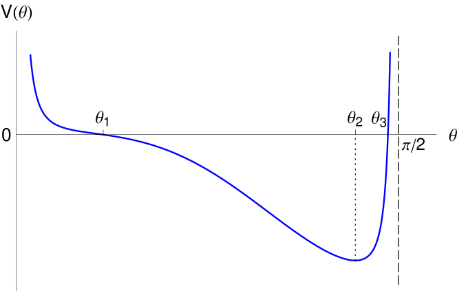
Figure 6: The potential $V(\theta)$ in Eq. (6.6) for $\Omega=5$ and $\kappa=0$.

To estimate the interaction time for the flavor current, we shall evaluate the time that the wave packet takes to travel from the boundary to the interior of the D7–brane, where it can excite mesons. A similar analysis for the case of the ${\cal R}$–current was presented in Ref. [27]. Near the boundary, where $\theta\ll 1$, the equation becomes

$$i\,\frac{\partial\Psi}{\partial\tau}\,\simeq\,\left(-\,\frac{1}{2\Omega}\,\frac{\partial^{2}}{\partial\theta^{2}}\,+\,\frac{3}{8\Omega}\frac{1}{\theta^{2}}\right)\Psi,$$ (6.8)

with the following, exact, solution ($C$ is a constant)

$$\Psi(\tau,\theta)\,=\,C\,\frac{\theta^{3/2}}{\tau^{2}}\ \exp\left(i\frac{\Omega\theta^{2}}{2\tau}\right)\,,$$ (6.9)

which describes diffusion : at early times, the penetration $\theta$ of the wave packet in the radial dimension grows with $\tau$ like

$$\theta(\tau)\,\sim\,\sqrt{\frac{2\tau}{\Omega}}\qquad\mbox{for}\quad\tau\,\lesssim\,\tau_{1}\,\sim\,\Omega^{1/3}\,.$$ (6.10)

Here $\tau_{1}$ is the time the wave takes to reach the point $\theta_{1}$, cf. Eq. (6.7), where the potential becomes attractive; in physical units, $\bar{t}_{1}\sim R_{0}\tau_{1}\sim\bar{k}^{1/3}$.

For $\tau>\tau_{1}$, and so long as $\theta$ lies in between $\theta_{1}$ and the minimum of the potential at $\theta_{2}$, the wave packet falls in the potential, essentially by following the classical equation of motion:

$$\Omega\,\frac{\partial^{2}\theta}{\partial\tau^{2}}\,=\,-\,\frac{\partial V}{\partial\theta}\,\simeq\,8\Omega\,\frac{\partial}{\partial\theta}\,\sin^{4}\theta\,.$$ (6.11)

For most of this travel, $\theta$ is still small, so $\sin^{4}\theta\simeq\theta^{4}$ and

$$\frac{\partial^{2}\theta}{\partial\tau^{2}}\,\simeq\,32\,\theta^{3}\ \Longrightarrow\ \theta(\tau)\,\simeq\,\frac{1}{1/\theta_{1}-4(\tau-\tau_{1})}\,.$$ (6.12)

So, the penetration $\theta$ becomes of $\mathcal{O}{(1)}$ at $\tau\sim\tau_{2}$, with

$$\tau_{2}-\tau_{1}\,\sim\,\frac{1}{4\theta_{1}}\,\sim\,\Omega^{1/3}\ \Longrightarrow\ \bar{t}_{2}-\bar{t}_{1}\,\sim\,\bar{t}_{1}\,\sim\,\bar{k}^{1/3}\,.$$ (6.13)

That is, it takes (parametrically) as much time to the wave to fall in the potential up to large distances $\theta\sim\mathcal{O}{(1)}$ as it takes to diffusively reach the attractive part of the potential, although the respective distances are very different: $\theta_{2}\gg\theta_{1}$. This is so because along the second part of the trajectory, from $\theta_{1}$ to $\theta_{2}$, the wave has un accelerated motion under the influence of the BH.

This time $\bar{t}_{2}\sim\bar{k}^{1/3}$ is already a realistic estimate for the interaction time, since the current can resonantly produce mesons when $\theta$ is of $\mathcal{O}{(1)}$. Moreover, this estimate would not change if the meson was to be produced further down in the worldvolume of the D7–brane (say, near its lower tip at $\theta\simeq\pi/2$), since the final part of the fall in the potential is very rapid because the potential is so attractive around $\theta_{2}$. We thus conclude that $\bar{t}_{\rm int}\sim\bar{k}^{1/3}$, as anticipated in Eq. (5.16). This also confirms that the typical uncertainties in the energy and the virtuality of the wave packet satisfy $\delta\bar{\omega}\gtrsim 1/\bar{k}^{1/3}$ and, respectively, $\delta\bar{Q}\gtrsim\bar{k}^{1/3}$, in agreement with our original assumptions.

Since determined by the dynamics relatively close to the Minkowski boundary, this interaction time is independent of $R_{0}$, and thus is parametrically the same as for the ${\cal R}$–current [27]. As we shall shortly see, a similar conclusion holds also for the light–like meson excitations with large quantum numbers $n\gg 1$ : such a meson has a period (the interval of time corresponding to one rotation around a semiclassical orbit) $\Delta\bar{t}_{n}\sim\bar{\omega}^{1/3}_{n}$ and spends most of this time at radial locations far away from $R_{0}$, namely around $\rho\sim n^{1/3}R_{0}$. The subsequent calculation will also shed light on an interesting property of the meson spectrum, which played an important role in our previous argument: the strong sensitivity of the dispersion relation to variations in the virtuality $\bar{Q}$ around the light–cone ($\bar{Q}=0$).

To that aim, we resort again on the Bohr–Sommerfeld quantization formula, valid for large $n$. We thus write

$$n\pi\,=\,\int_{\theta_{1}}^{\theta_{3}}{\rm d}\theta\,p(\theta\,;E_{n},\Omega)\,,\qquad p(\theta\,;E,\Omega)\,\equiv\,\sqrt{2\Omega(E-V(\Omega))}\,,$$ (6.14)

where $E_{n}$ are the energy levels associated with the Schrödinger Hamiltonian in Eq. (6.5). These energies are defined by the usual eigenvalue problem $H\Psi_{n}=E_{n}\Psi_{n}$ and depend upon the two parameters $\Omega$ and $\kappa$ within $H$. They should not be confused with the meson energies $\Omega_{n}$, which rather correspond to the special values of $\Omega$ (at a given $\kappa$) for which the homogeneous equation $H\Psi=0$ has non–trivial, normalizable, solutions. One clearly has

$$E_{n}(\Omega,\kappa)\,=\,0\qquad\mbox{for}\qquad\Omega=\Omega_{n}(\kappa)\,.$$ (6.15)

This last equation has a unique solution for any $n=0,1,2,...$, as it can be easily recognized by inspection of the potential in Eq. (6.6) and Fig. 6. By choosing $E_{n}=0$ in Eq. (6.14), one could work out the corresponding integral and thus recover our previous result that, e.g., $\Omega_{n}(\kappa)=n$, cf. Eq. (4.15). However, for the present purposes, we shall rather use Eq. (6.14) to compute the level spacing of the Schrödinger energies near $E=0$, that is

$$\Delta E(\Omega_{n})\,\equiv\,E_{n+1}(\Omega_{n})-E_{n}(\Omega_{n})\,=\,E_{n}(\Omega_{n})\qquad(\kappa\,=\,0)\,.$$ (6.16)

Using Eq. (6.14), this is obtained as (we anticipate that $\Delta E\ll 1$)

$$\pi\,=\,\int_{\theta_{1}}^{\theta_{3}}{\rm d}\theta\,\big{[}p(\theta\,;\Delta E,\Omega_{n})-p(\theta\,;0,\Omega_{n})\big{]}\,\simeq\,\Delta E\int_{\theta_{1}}^{\theta_{3}}{\rm d}\theta\,\frac{\partial p}{\partial E}\Bigg{|}_{E=0}\,=\,\Delta E\int_{\theta_{1}}^{\theta_{3}}{\rm d}\theta\,\frac{\Omega_{n}}{p}\,.$$ (6.17)

Indeed, this quantity $\Delta E(\Omega_{n})$ provides the answer to the two questions that we are interested in, as we explain now:

(i) The last integral in Eq. (6.17) is the same as half of the period for a round trip around a semiclassical orbit: indeed, $p=\Omega\partial_{\tau}\theta$, hence $(\Omega/p){\rm d}\theta={\rm d}\tau$.

(ii) The quantity $\Delta E(\Omega_{n})$ characterizes the response of the meson dispersion relation to variations in the meson virtuality near the light–cone. This can be understood by recalling the discussion below Eq. (6.6), about the last term, ${\kappa^{2}}/{2\Omega}$, in the potential. More precisely, $\Delta E(\Omega_{n})$ is a measure of the increase in the virtuality which is needed to jump from one meson level ($n+1$) to the neighboring one ($n$) at fixed energy and in the vicinity of the light–cone. In formulæ, $\Delta E(\Omega_{n})={\kappa^{2}_{n}}/{2\Omega_{n}}$ with $\kappa_{n}$ defined by $\Omega_{n+1}(0)=\Omega_{n}(\kappa_{n})$, or

$$E_{n}(\Omega_{n}(\kappa_{n}),\kappa_{n})\,=\,E_{n+1}(\Omega_{n}(\kappa_{n}),0)\,=\,0\,.$$ (6.18)

Returning to Eq. (6.17), this can be evaluated as

$$\frac{\pi}{\Delta E} \,\simeq\, \frac{1}{4}\int_{\theta_{1}}^{\theta_{3}}{\rm d}\theta\,\left({\sin^{4}\theta\,-\,\frac{3}{64\Omega_{n}^{2}}\,\frac{1}{\sin^{2}\theta\cos^{2}\theta}}\right)^{-1/2}$$

$$\,\simeq\, \frac{1}{4}\int_{\theta_{1}}^{\infty}\,\frac{{\rm d}\theta\,\theta}{\sqrt{\theta^{6}-\theta^{6}_{1}}}\,=\,\frac{1}{24\theta_{1}}\,{\rm B}(1/6,1/2)\,,$$

where in the second line we have used the fact that the integral is dominated by its lower limit $\theta_{1}\ll 1$, and ${\rm B}(1/6,1/2)$ is the respective Beta function.

We thus find that the period for motion of a meson around the semiclassical orbit with quantum number $n$ is $\Delta\bar{t}_{n}\sim 1/\theta_{1}\sim\bar{\omega}^{1/3}_{n}$. Moreover, the fact that the above integral is dominated by $\theta\sim\theta_{1}$ also means that a quantum particle in the bound state with energy $E_{n}\simeq 0$ spends most of its time at relatively large radial distances $\rho\sim\bar{\omega}^{1/3}_{n}\sim n^{1/3}R_{0}$. This implies a similar property for the light–like meson with energy $\bar{\omega}_{n}\simeq\sqrt{2}nR_{0}^{3}$. Of course, the meson wavefunction has support everywhere in the range $R_{0}\lesssim\rho\lesssim n^{1/3}R_{0}$, but the radial velocity $\partial_{\tau}\theta$ is smaller towards the upper end of this range (as it should be clear by inspection of the potential in Fig. 6), therefore there is a larger probability to find the meson in that region than towards the bottom of the D7–brane.

Furthermore, the result for $\Delta E$ in Eq. (6) implies

$$\Delta E(\Omega_{n})\,\equiv\,\frac{\kappa^{2}_{n}}{2\Omega_{n}}\,\sim\,\frac{1}{\theta_{1}}\quad\Longrightarrow\quad\kappa^{2}_{n}\,\sim\,\Omega_{n}^{2/3}\,,$$ (6.20)

or $\bar{Q}_{n}\sim\bar{\omega}_{n}^{1/3}$. This is in agreement with our previous discussion of Eq. (4.17) in Sect. 4.3 : there is enough to make a rather small change $\Delta\bar{Q}_{n}\sim n^{1/3}R_{0}$ in the meson virtuality in order to jump from one mode to another at fixed energy, whereas one needs a substantially larger increase in the energy of the meson, namely $\Delta\bar{\omega}_{n}\sim R_{0}^{3}$, in order to make that jump at fixed virtuality. The above result for $\bar{Q}_{n}$ is moreover of the same order as the fluctuations $\delta\bar{Q}$ in the virtuality of the flavor current due to its energy uncertainty, thus justifying the energy averaging performed in our previous calculation of the spectral weight, in Eq. (5.18).

Appendix A WKB approach to light–like mesons

In this appendix, we shall use the WKB approximation to rederive the results in Sect. 5.1 on the spectrum and the wavefunctions of the light–like mesons in the limit of a large quantum number $n\gg 1$. We have already noticed in Sect. 4.3 that the WKB method correctly reproduces the spectrum (5.10) except for the constant shift 1/6 in the eigenvalues $\Omega_{n}$ (which is of course a subdominant term at large $n$). As we shall see, this constant shift is also the only source of deviation between the WKB eigenfunctions and the asymptotic expansion of the corresponding exact result, as given by Eq. (5.7).

Specifically, let us view Eq. (5.1) as the Schrödinger equation for a non–relativistic quantum mechanical particle in a stationary state with energy $E=0$. We recall that the potential in that equation becomes infinite at the end point $\zeta=1$ (cf. Fig. 4 right). Then for $\zeta<1$, the associated wavefunction can be obtained in the WKB approximation as [56]

$$\psi(\zeta)\,=\,\frac{C}{\sqrt{p(\zeta)}}\,\sin\left(\int_{\zeta}^{1}{\rm d}\zeta^{\prime}\,p(\zeta^{\prime})\,+\,\alpha\right)\,,\qquad p(\zeta)\,\equiv\,\sqrt{-V(\zeta)}\,.$$ (A.21)

The shift $\alpha$ in the argument of the sine function is not accurately determined by the WKB method, but will be later fixed by matching onto the exact solution near $\zeta=1$. With the potential $V(\zeta)$ in Eq. (5.1), the integral in Eq. (A.21) is straightforward and yields

$$\psi(\zeta)\,=\,C^{\prime}\left(\frac{\zeta}{1-\zeta}\right)^{1/4}\,\sin\left[2\Omega\left(\frac{\pi}{2}-\arcsin\sqrt{\zeta}-\sqrt{\zeta(1-\zeta)}\right)\,+\,\alpha\right]\,.$$ (A.22)

This solution is not reliable very close to the end points at $\zeta=0$ (where the potential becomes singular) and $\zeta=1$ (where the potential is not differentiable), but it should be a reasonable approximation at the intermediate points. A similar WKB solution can be constructed on the right of $\zeta=0$. The condition that the two solutions match with each other at intermediate points leads to the Bohr–Sommerfeld quantization condition (4.14), which in turn implies $\Omega_{n}\approx n$ when $n\gg 1$. With $\Omega_{n}=n$, the WKB solution (A.22) has exactly $n$ nodes in between 0 and 1.

When approaching the end point at $\zeta=1$, we expect Eq. (A.22) to remain a good approximation so long as [56]

$$(1-\zeta)^{3/2}\,\gg\,\frac{1}{\sqrt{-{\rm d}V/{\rm d}\zeta}}\,=\,\frac{1}{2\Omega}\,,$$ (A.23)

where $-{\rm d}V/{\rm d}\zeta=4\Omega^{2}$ is the left derivative of the potential at $\zeta=1$. This range of validity, which in terms of the variable $\xi$ introduced in Eq. (5.6) amounts to $\xi\gg 1$, is wide enough to allow for a matching between the WKB solution and the exact solution near $\zeta=1$. The latter is the following linear combination of Airy functions

$$\psi_{\rm b}(\xi)\,\simeq\,\frac{\sqrt{3}}{2}\,{\rm Ai}(-\xi)\,-\,\frac{1}{2}\,{\rm Bi}(-\xi)\qquad\mbox{for \ \ $0\,\leq\,\xi\,\ll\,(2\Omega)^{{2}/{3}}$}\,,$$ (A.24)

where the relative coefficient has been fixed by the condition that $\psi=0$ when $\xi=0$. Clearly, Eqs. (A.22) and (A.24) have a common validity domain at $1\ll\xi\ll(2\Omega)^{{2}/{3}}$, and within that domain they are indeed consistent with each other, as we now check.

To that aim, we need to compare the approximate form of Eq. (A.24) valid at $\xi\gg 1$, which is obtained similarly to Eq. (5.8) and reads

$$\psi_{\rm b}(\xi)\,\simeq\,\frac{C}{\xi^{1/4}}\,\sin\left(\frac{2}{3}\,\xi^{3/2}\,+\frac{\pi}{12}\right),$$ (A.25)

to the approximate form of Eq. (A.22) valid near $\zeta=1$ (i.e., for $\xi\ll(2\Omega)^{{2}/{3}}$), which is readily obtained as

$$\psi(\xi)\,\simeq\,\frac{C}{\xi^{1/4}}\,\sin\left(\frac{2}{3}\,\xi^{3/2}\,+\,\alpha\right)\,.$$ (A.26)

Clearly, these two expressions, (A.25) and (A.26), are consistent with each other, as anticipated. Moreover they perfectly match provided one choses $\alpha=\pi/12$, thus completely fixing the WKB solution (A.22), valid for any $\zeta$ which obeys the condition (A.23) and which is not too close to $\zeta=0$.

References

- [1] O. Aharony, S. S. Gubser, J. M. Maldacena, H. Ooguri, and Y. Oz, “Large N field theories, string theory and gravity,” Phys. Rept. 323 (2000) 183–386, arXiv:hep-th/9905111.
- [2] D. T. Son and A. O. Starinets, “Viscosity, Black Holes, and Quantum Field Theory,” Ann. Rev. Nucl. Part. Sci. 57 (2007) 95–118, arXiv:0704.0240 [hep-th].
- [3] E. Iancu, “Partons and jets in a strongly-coupled plasma from AdS/CFT,” Acta Phys. Polon. B39 (2008) 3213–3280, arXiv:0812.0500 [hep-ph].
- [4] J. Erdmenger, N. Evans, I. Kirsch, and E. Threlfall, “Mesons in Gauge/Gravity Duals - A Review,” Eur. Phys. J. A35 (2008) 81–133, arXiv:0711.4467 [hep-th].
- [5] S. S. Gubser, S. S. Pufu, F. D. Rocha, and A. Yarom, “Energy loss in a strongly coupled thermal medium and the gauge-string duality,” arXiv:0902.4041 [hep-th].
- [6] M. Rangamani, “Gravity & Hydrodynamics: Lectures on the fluid-gravity correspondence,” Class. Quant. Grav. 26 (2009) 224003, arXiv:0905.4352 [hep-th].
- [7] C. P. Herzog, A. Karch, P. Kovtun, C. Kozcaz, and L. G. Yaffe, “Energy loss of a heavy quark moving through N = 4 supersymmetric Yang-Mills plasma,” JHEP 07 (2006) 013, hep-th/0605158.
- [8] S. S. Gubser, “Drag force in AdS/CFT,” Phys. Rev. D74 (2006) 126005, hep-th/0605182.
- [9] H. Liu, K. Rajagopal, and U. A. Wiedemann, “Calculating the jet quenching parameter from AdS/CFT,” Phys. Rev. Lett. 97 (2006) 182301, hep-ph/0605178.
- [10] J. Casalderrey-Solana and D. Teaney, “Heavy quark diffusion in strongly coupled N = 4 Yang Mills,” Phys. Rev. D74 (2006) 085012, hep-ph/0605199.
- [11] S. S. Gubser, “Momentum fluctuations of heavy quarks in the gauge-string duality,” Nucl. Phys. B790 (2008) 175–199, arXiv:hep-th/0612143.
- [12] J. Casalderrey-Solana and D. Teaney, “Transverse momentum broadening of a fast quark in a N = 4 Yang Mills plasma,” JHEP 04 (2007) 039, hep-th/0701123.
- [13] S. S. Gubser, S. S. Pufu, and A. Yarom, “Energy disturbances due to a moving quark from gauge- string duality,” JHEP 09 (2007) 108, arXiv:0706.0213 [hep-th].
- [14] P. M. Chesler and L. G. Yaffe, “The stress-energy tensor of a quark moving through a strongly-coupled N=4 supersymmetric Yang-Mills plasma: comparing hydrodynamics and AdS/CFT,” arXiv:0712.0050 [hep-th].
- [15] F. Dominguez, C. Marquet, A. H. Mueller, B. Wu, and B.-W. Xiao, “Comparing energy loss and -broadening in perturbative QCD with strong coupling SYM theory,” Nucl. Phys. A811 (2008) 197–222, arXiv:0803.3234 [nucl-th].
- [16] G. C. Giecold, E. Iancu, and A. H. Mueller, “Stochastic trailing string and Langevin dynamics from AdS/CFT,” JHEP 07 (2009) 033, arXiv:0903.1840 [hep-th].
- [17] K. Peeters, J. Sonnenschein, and M. Zamaklar, “Holographic melting and related properties of mesons in a quark gluon plasma,” Phys. Rev. D74 (2006) 106008, hep-th/0606195.
- [18] H. Liu, K. Rajagopal, and U. A. Wiedemann, “An AdS/CFT calculation of screening in a hot wind,” Phys. Rev. Lett. 98 (2007) 182301, hep-ph/0607062.
- [19] M. Chernicoff, J. A. Garcia, and A. Guijosa, “The energy of a moving quark-antiquark pair in an N = 4 SYM plasma,” JHEP 09 (2006) 068, hep-th/0607089.
- [20] E. Caceres, M. Natsuume, and T. Okamura, “Screening length in plasma winds,” JHEP 10 (2006) 011, hep-th/0607233.
- [21] P. C. Argyres, M. Edalati, and J. F. Vazquez-Poritz, “No-drag string configurations for steadily moving quark- antiquark pairs in a thermal bath,” JHEP 01 (2007) 105, hep-th/0608118.
- [22] Q. J. Ejaz, T. Faulkner, H. Liu, K. Rajagopal, and U. A. Wiedemann, “A limiting velocity for quarkonium propagation in a strongly coupled plasma via AdS/CFT,” JHEP 04 (2008) 089, arXiv:0712.0590 [hep-th].
- [23] D. Mateos, R. C. Myers, and R. M. Thomson, “Thermodynamics of the brane,” JHEP 05 (2007) 067, arXiv:hep-th/0701132.
- [24] C. Hoyos-Badajoz, K. Landsteiner, and S. Montero, “Holographic Meson Melting,” JHEP 04 (2007) 031, arXiv:hep-th/0612169.
- [25] R. C. Myers, A. O. Starinets, and R. M. Thomson, “Holographic spectral functions and diffusion constants for fundamental matter,” JHEP 11 (2007) 091, arXiv:0706.0162 [hep-th].
- [26] Y. Hatta, E. Iancu, and A. H. Mueller, “Deep inelastic scattering off a N=4 SYM plasma at strong coupling,” JHEP 01 (2008) 063, arXiv:0710.5297 [hep-th].
- [27] Y. Hatta, E. Iancu, and A. H. Mueller, “Jet evolution in the N=4 SYM plasma at strong coupling,” JHEP 05 (2008) 037, arXiv:0803.2481 [hep-th].
- [28] S. Caron-Huot, P. Kovtun, G. D. Moore, A. Starinets, and L. G. Yaffe, “Photon and dilepton production in supersymmetric Yang- Mills plasma,” JHEP 12 (2006) 015, hep-th/0607237.
- [29] D. Mateos and L. Patino, “Bright branes for strongly coupled plasmas,” JHEP 11 (2007) 025, arXiv:0709.2168 [hep-th].
- [30] J. Casalderrey-Solana and D. Mateos, “Prediction of a Photon Peak in Relativistic Heavy Ion Collisions,” Phys. Rev. Lett. 102 (2009) 192302, arXiv:0806.4172 [hep-ph].
- [31] C. A. B. Bayona, H. Boschi-Filho, and N. R. F. Braga, “Deep inelastic scattering off a plasma with flavour from D3-D7 brane model,” arXiv:0912.0231 [hep-th].
- [32] J. Polchinski and M. J. Strassler, “Deep inelastic scattering and gauge/string duality,” JHEP 05 (2003) 012, hep-th/0209211.
- [33] Y. Hatta, E. Iancu, and A. H. Mueller, “Deep inelastic scattering at strong coupling from gauge/string duality : the saturation line,” JHEP 01 (2008) 026, arXiv:0710.2148 [hep-th].
- [34] C. A. Ballon Bayona, H. Boschi-Filho, and N. R. F. Braga, “Deep inelastic structure functions from supergravity at small x,” JHEP 10 (2008) 088, arXiv:0712.3530 [hep-th].
- [35] J. L. Albacete, Y. V. Kovchegov, and A. Taliotis, “DIS on a Large Nucleus in AdS/CFT,” JHEP 07 (2008) 074, arXiv:0806.1484 [hep-th].
- [36] A. H. Mueller, A. I. Shoshi, and B.-W. Xiao, “Deep inelastic and dipole scattering on finite length hot SYM matter,” Nucl. Phys. A822 (2009) 20–40, arXiv:0812.2897 [hep-th].
- [37] E. Avsar, E. Iancu, L. McLerran, and D. N. Triantafyllopoulos, “Shockwaves and deep inelastic scattering within the gauge/gravity duality,” JHEP 11 (2009) 105, arXiv:0907.4604 [hep-th].
- [38] F. Dominguez, “Particle production in DIS off a shockwave in AdS,” arXiv:0912.1641 [hep-th].
- [39] E. Iancu and A. H. Mueller, “A lattice test of strong coupling behaviour in QCD at finite temperature,” Phys. Lett. B681 (2009) 247–252, arXiv:0906.3175 [hep-ph].
-
[40]
A.H. Mueller, Parton Saturation–An Overview, hep-ph/0111244;
E. Iancu, A. Leonidov and L. McLerran, The Colour Glass Condensate: An Introduction, hep-ph/0202270. Published in QCD Perspectives on Hot and Dense Matter, Eds. J.-P. Blaizot and E. Iancu, NATO Science Series, Kluwer, 2002. - [41] A. Karch and E. Katz, “Adding flavor to AdS/CFT,” JHEP 06 (2002) 043, arXiv:hep-th/0205236.
- [42] J. Babington, J. Erdmenger, N. J. Evans, Z. Guralnik, and I. Kirsch, “Chiral symmetry breaking and pions in non-supersymmetric gauge / gravity duals,” Phys. Rev. D69 (2004) 066007, arXiv:hep-th/0306018.
- [43] M. Kruczenski, D. Mateos, R. C. Myers, and D. J. Winters, “Meson spectroscopy in AdS/CFT with flavour,” JHEP 07 (2003) 049, arXiv:hep-th/0304032.
- [44] D. Mateos, R. C. Myers, and R. M. Thomson, “Holographic phase transitions with fundamental matter,” Phys. Rev. Lett. 97 (2006) 091601, arXiv:hep-th/0605046.
- [45] A. Mocsy, “Quarkonium Spectral Functions,” Nucl. Phys. A830 (2009) 411c–418c, arXiv:0908.0746 [hep-ph].
- [46] H. T. Ding, O. Kaczmarek, F. Karsch, H. Satz, and W. Soeldner, “Charmonium correlators and spectral functions at finite temperature,” arXiv:0910.3098 [hep-lat].
- [47] J. M. Maldacena, “The large N limit of superconformal field theories and supergravity,” Adv. Theor. Math. Phys. 2 (1998) 231–252, hep-th/9711200.
- [48] S. S. Gubser, I. R. Klebanov, and A. M. Polyakov, “Gauge theory correlators from non-critical string theory,” Phys. Lett. B428 (1998) 105–114, hep-th/9802109.
- [49] E. Witten, “Anti-de Sitter space and holography,” Adv. Theor. Math. Phys. 2 (1998) 253–291, hep-th/9802150.
- [50] E. Witten, “Anti-de Sitter space, thermal phase transition, and confinement in gauge theories,” Adv. Theor. Math. Phys. 2 (1998) 505–532, hep-th/9803131.
- [51] L. Alvarez-Gaume and S. F. Hassan, “Introduction to S-duality in N = 2 supersymmetric gauge theories: A pedagogical review of the work of Seiberg and Witten,” Fortsch. Phys. 45 (1997) 159–236, arXiv:hep-th/9701069.
- [52] C. Fefferman and R. C. Graham, “Conformal Invariants”, in “Elie Cartan et les Mathematiques d’aujourd’hui”. Paris, Asterisque (1985) 95.
- [53] D. T. Son and A. O. Starinets, “Minkowski-space correlators in AdS/CFT correspondence: Recipe and applications,” JHEP 09 (2002) 042, hep-th/0205051.
- [54] C. P. Herzog and D. T. Son, “Schwinger-Keldysh propagators from AdS/CFT correspondence,” JHEP 03 (2003) 046, hep-th/0212072.
- [55] M. Abramowitz and I. A. Stegun, “Handbook of Mathematical Functions with Formulas, Graphs, and Mathematical Tables”. New York, Dover (1965).
- [56] L. Landau and E. Lifchitz, “Quantum mechanics : non-relativistic theory”. New York, Pergamon Press (1981).