Summary

We consider a family $S=S(a)$ of $2$-valued transformations of special form on the segment $[0,1]$ with measure $\mu={\displaystyle\int}p(x)\,d\lambda$, which is absolutely continuous with respect to the Lebesgue measure $\lambda$. We endow $S$ with a set of weight functions $\alpha=\{\alpha_{1}(x),\alpha_{2}(x)\}$ and find a criterion of measure invariance under the transformation. This criterion relates the three parameters $a$, $p$, $\alpha$ to each other.

Key words: multivalued dynamical system, invariant measure, $\beta$-expansion, Bernoulli convolution

Аннотация

Рассматривается семейство двузначных трансформаций $S=S(a)$ специального вида на отрезке $[0,1]$ с мерой $\mu={\displaystyle\int}p(x)\,d\lambda$, абсолютно непрерывной относительно меры Лебега $\lambda$. Трансформация $S$ оснащается набором весовых функций $\alpha=\{\alpha_{1}(x),\alpha_{2}(x)\}$. Находится критерий инвариантности меры под действием заданной оснащенной трансформации. Этот критерий явным образом связывает три параметра: $a$, $p$ и $\alpha$.

Ключевые слова: многозначная динамическая система, инвариантная мера, $\beta$-разложение

 

1 Introduction. Dynamical system connected to arithmetic representation

Connections between the ergodic theory and the metric number theory are well known. One of these connections are arithmetic representations arising in special symbolic realization of dynamical systems.

Let $\beta\in(1,2]$. Any infinite sequence $\sigma_{1}\sigma_{2}\ldots$ of zeros and ones is called $\beta$-expansion of number $x\in[0,1]$ (see [1, 2]), provided that

$$x=\sum_{k=1}^{\infty}\sigma_{k}\beta^{-k}.$$

It is clear that with $\beta=2$ we obtain the usual binary representation of number $x$.

Every number $x\in[0,1]$ has at least one $\beta$-expansion which is called canonical, or <<greedy expansion>>: $\sigma_{k}=[\beta T^{k-1}x]$, $k\geq 1$, where $Tx=\{\beta x\}$ ($[y]$ and $\{y\}$ — whole and fractional parts of number $y\in\mathbb{R}$) (see [3]).

If $\beta\in\left(1,\frac{1+\sqrt{5}}{2}\right)$, then $x\in[0,1]$ has a continuum of different $\beta$-expansions [4], if $\beta\in\left[\frac{1+\sqrt{5}}{2},2\right)$, the same is true for almost every $x\in[0,1]$  [5]. On the other hand, for all $m\in\mathbb{N}$ there exists a base $\beta\in\left(\frac{1+\sqrt{5}}{2},2\right)$ and a number $x\in[0,1]$ which has exactly $m$ different $\beta$-expansions [6].

As it is shown in [7], to find an arbitrary $\beta$-expansion of number $x_{1}\in[0,1]$, it is necessary and sufficient to follow the one of the possible orbit of the point $x_{1}$ under multi-valued transformation $S$ (see fig. 1)

$$\begin{cases}h_{0}(x)=\beta x,&x\in\left[0,\frac{1}{\beta}\right];\\[5.69046pt] h_{1}(x)=\beta x-\beta+1,&x\in\left[1-\frac{1}{\beta},1\right].\end{cases}$$

There is a correspondence between every orbit $x_{1},x_{2},x_{3}\ldots$ and $\beta$-expansion $\sigma_{1}\sigma_{2}\sigma_{3}\ldots$ of number $x_{1}$ which can be found by the rule:

$$\sigma_{k}=0,\mbox{ \T2A\cyre\T2A\cyrs\T2A\cyrl\T2A\cyri }x_{k+1}=h_{0}(x_{k});$$

$$\sigma_{k}=1,\mbox{ \T2A\cyre\T2A\cyrs\T2A\cyrl\T2A\cyri }x_{k+1}=h_{1}(x_{k}).$$

If $x_{k}\in[1-\frac{1}{\beta},\frac{1}{\beta}]$, then we can choose the mapping $h_{0}$ as well as $h_{1}$ to construct $x_{k+1}$. Thus we obtain every possible $\beta$-expansions of number $x_{1}$.

To find a canonical $\beta$-expansion it is necessary and sufficient to follow in the same way as before a single-valued orbit under $1$-transformation $S_{2}$ (see fig. 1)

$$S_{2}(x)=\begin{cases}\beta x,&x\in\left[0,1-\frac{1}{\beta}\right);\\[5.69046pt] \beta x-\beta+1,&x\in\left[1-\frac{1}{\beta},1\right].\end{cases}$$

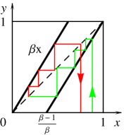
Figure 1: Scheme of transformations $S$ (on the left) and $S_{2}$ (on the right)

By investigating the orbits of points under transformation $S_{2}$, we come to the conclusion that orbits of all the points except $x=1$ are <<captured>> by the segment $[0,\beta-1]$. Dynamical system $([0,\beta-1];S_{2}|_{[0,\beta-1]})$ was considered in classical papers on $\beta$-expansions [1, 8, 2], in which they found invariant measure equivalent to the Lebesgue measure, and also in [9, 7], where they calculated top addresses for the iterated function system $\left\{[0,1];\phi_{1}(x)=\frac{1}{\beta}x+1-\frac{1}{\beta},\phi_{2}(x)=\frac{1}{\beta}x,\quad 1<\beta<2\right\}$.

Transformation $S$ is also tightly connected to the problem of finding every parameter $\beta\in(1,2)$ which provides nonsingularity of Erdős measure on the segment $[0,1]$, — а measure corresponding to a distribution of random variable $\sum_{k=1}^{\infty}\sigma_{k}\beta^{-k}$ where coefficients $\sigma_{k}\in\{0,1\}$ are independently chosen with probability $1/2$ (this is called Bernoulli convolution problem and it has not been solved yet) (see [10], fine survey on the topic can be found in [11]).

Given $a\in\left.\left(0,\frac{1}{2}\right.\right]$, we consider $2$-transformation $S=S_{1}\cup S_{2}$ on the segment $[0,1]$ (see fig. 2) where
$S_{1}(x)=\begin{cases}\frac{1}{1-a}x,&x\in[0,1-a);\cr\frac{1}{1-a}x-\frac{a}{1-a},&x\in[1-a,1],\cr\end{cases}$ $\quad S_{2}(x)=\begin{cases}\frac{1}{1-a}x,&x\in[0,a);\cr\frac{1}{1-a}x-\frac{a}{1-a},&x\in[a,1].\cr\end{cases}$

Note that in the discussion above $\beta=\frac{1}{1-a}$.

$=$

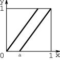
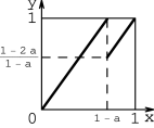
$\bigcup$

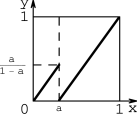
Figure 2: Scheme of $2$-transformation $S=S_{1}\cup S_{2}$

Let $\lambda$ be the Lebesgue measure on $[0,1]$, $\mathfrak{B}$ — $\sigma$-field of Borel subsets of $[0,1]$. Let also $\mu(B)=\int_{B}p(x)\,d\lambda$ be a measure absolutely continuous with respect to the Lebesgue measure, $p(x)\in L^{1}([0,1],\mathfrak{B},\lambda)$ and $p(x)\geq 0$. We endow $2$-transformation $S$ with a set of weight functions

$$\alpha=\{\alpha_{1}(x),\alpha_{2}(x)\},\quad\alpha_{1}(x),\alpha_{2}(x)\in L^{1}([0,1],\mathfrak{B},\lambda)$$

provided that $\alpha_{1}(x)+\alpha_{2}(x)\equiv 1$ and $\alpha_{1}(x),\alpha_{2}(x)\geq 0$. Henceforth, we consider $2$-valued dynamical system $([0,1],\mathfrak{B},\mu,\{S,\alpha\})$ with the finite measure $\mu$.

According to [12], we obtain a new measure $\mu_{S}$ on $\mathfrak{B}$ by the next formula:

$$\mu_{S}(B)=\int\limits_{S_{1}^{-1}(B)}\alpha_{1}(x)p(x)\,d\lambda+\int\limits_{S_{2}^{-1}(B)}\alpha_{2}(x)p(x)\,d\lambda.$$

Denote $\alpha_{1}(x)p(x)=A_{1}(x)$, $\alpha_{2}(x)p(x)=A_{2}(x)$. Then $A_{1}(x)+A_{2}(x)=p(x)$ and

$$\mu_{S}(B)=\int\limits_{S_{1}^{-1}(B)}A_{1}(x)\,d\lambda+\int\limits_{S_{2}^{-1}(B)}A_{2}(x)\,d\lambda.$$

There are three independent parameters in the studied construction: density function $p(x)$, number $a$ (parameter of transformation $S$) and an equipment $\alpha=\{\alpha_{1}(x),\alpha_{2}(x)\}$ ($\mu=\mu(p)$ and $S=S(a,\alpha)$). When searching for equipped transformation with given invariant measure $\mu$ or searching measure which is preserved by given transformation $S$, — we have a certain relation between the parameters to fulfill the equation $\mu_{S}=\mu$.

This relation is investigated in Lemma 1 and Theorem 2. In the Corollary 2 we particularly discuss the Lebesgue measure($p\equiv 1$). The construction defined in Theorem 2 gives an example of an invariant measure with non-constant density. Two more examples consistent with classical results in ergodic theory are given in Corollaries 2 and 2.

2 Main results. Criterion of measure invariance

Fix three parameters: $a\in\left.\left(0,\frac{1}{2}\right.\right]$, $\alpha=\{\alpha_{1}(x),\alpha_{2}(x)\}$ and $p(x)$. Then the condition of measure invariance $\mu_{S}=\mu$ is characterized by the following

$\mu_{S}=\mu$ if and only if for almost every $x\in[0,1]$ (with respect to $\lambda$)

$$A_{1}((1-a)x)+\chi_{\left[\frac{1-2a}{1-a},1\right]}(x)A_{1}((1-a)x+a)+A_{2}((1-a)x+a)+\\ +\chi_{\left[\left.0,\frac{a}{1-a}\right.\right)}(x)A_{2}((1-a)x)=\frac{p(x)}{1-a}.$$ (1)

      Proof. .

Let $C_{1}=\left[\frac{1-2a}{1-a},1\right]$, $C_{2}=\left[\left.0,\frac{a}{1-a}\right.\right)$. Then by changing variables in the Lebesgue integral we obtain that for every $B\in\mathfrak{B}$

$$\mu_{S}(B)=\int\limits_{(1-a)B}A_{1}(x)\,d\lambda+\int\limits_{(1-a)(B\cap C_{1})+a}A_{1}(x)\,d\lambda+\int\limits_{(1-a)(B\cap C_{2})}A_{2}(x)\,d\lambda+\\ +\int\limits_{(1-a)B+a}A_{2}(x)\,d\lambda=\\ =(1-a)\left(\int\limits_{B}A_{1}((1-a)x)\,d\lambda+\int\limits_{B}\chi_{C_{1}}(x)A_{1}((1-a)x+a)\,d\lambda+\right.\\ \left.+\int\limits_{B}\chi_{C_{2}}(x)A_{2}((1-a)x)\,d\lambda+\int\limits_{B}A_{2}((1-a)x+a)\,d\lambda\right).$$ (2)

If $\mu_{S}=\mu$, then considering arbitrariness of $B\in\mathfrak{B}$ formula (2) implies (1). And conversely, by substituting the equality (1) into (2), we get $\mu_{S}=\mu$. ∎

Let henceforward

$$\frac{1}{n+1}<a\leq\frac{1}{n}\qquad(n\in\mathbb{N},n\geq 2).$$

$\mu_{S}=\mu$ if and only if the following conditions hold true:

$$\sum\limits_{k=-1}^{n-1}p(x_{0}+ka)=\frac{1}{1-a}\sum\limits_{k=-1}^{n-2}p\!\left(\frac{x_{0}+ka}{1-a}\right),\quad x_{0}\in[a,1-(n-1)a);$$ (3)

$$\sum\limits_{k=-1}^{n-2}p(x_{1}+ka)=\frac{1}{1-a}\sum\limits_{k=-1}^{n-3}p\!\left(\frac{x_{1}+ka}{1-a}\right),\quad x_{1}\in[1-(n-1)a,2a);$$ (4)

$$\alpha_{1}(x+ma)p(x+ma)=\sum\limits_{k=-1}^{m}p(x+ka)-\frac{1}{1-a}\sum\limits_{k=-1}^{m-1}p\!\left(\frac{x+ka}{1-a}\right),$$ (5)

where $x+ma\in[(m+1)a,(m+2)a)$ for $m=\overline{0,n-3}$, $x+(n-2)a\in[(n-1)a,1-a)$.

There is no restriction on function $\alpha_{1}(x)$ on the intervals $[0,a)$ and $[1-a,1]$.

      Proof. .

Let us consider two cases.

1. First let $0<a\leq\frac{1}{3}$. Then $\frac{a}{1-a}\leq\frac{1-2a}{1-a}$ and formula (1) can be written in the following form:

$$\frac{p(x)}{1-a}=\begin{cases}p((1-a)x)+A_{2}((1-a)x+a),&x\in\left[\left.0,\frac{a}{1-a}\right.\right);\\[5.69046pt] A_{1}((1-a)x)+A_{2}((1-a)x+a),&x\in\left[\left.\frac{a}{1-a},\frac{1-2a}{1-a}\right.\right);\\[5.69046pt] p((1-a)x+a)+A_{1}((1-a)x),&x\in\left[\frac{1-2a}{1-a},1\right].\end{cases}$$ (6)

Consider the first equation of the system: $\frac{p(x)}{1-a}=p((1-a)x)+A_{2}((1-a)x+a)$, $x\in\left[\left.0,\frac{a}{1-a}\right.\right)$. Make a change $y=(1-a)x+a$, then, for $y\in[a,2a)$,

$$\frac{1}{1-a}\;p\!\left(\frac{y-a}{1-a}\right)=p(y-a)+A_{2}(y)=p(y-a)+p(y)-A_{1}(y).$$

Consider the second equation of the system: $\frac{p(x)}{1-a}=A_{1}((1-a)x)+A_{2}((1-a)x+a)$, $x\in\left[\left.\frac{a}{1-a},\frac{1-2a}{1-a}\right.\right)$. Make a change $y=(1-a)x$, then, for $y\in[a,1-2a)$,

$$\frac{1}{1-a}\;p\!\left(\frac{y}{1-a}\right)=A_{1}(y)+A_{2}(y+a)=p(y+a)+A_{1}(y)-A_{1}(y+a).$$

Consider the third equation of the system: $\frac{p(x)}{1-a}=p((1-a)x+a)+A_{1}((1-a)x)$, $x\in\left[\frac{1-2a}{1-a},1\right]$. Make a change $y=(1-a)x$, then, for $y\in[1-2a,1-a]$,

$$\frac{1}{1-a}\;p\!\left(\frac{y}{1-a}\right)=p(y+a)+A_{1}(y).$$

Thus we obtain:

$$\begin{cases}A_{1}(y)=p(y-a)+p(y)-\frac{1}{1-a}\;p\!\left(\frac{y-a}{1-a}\right),&y\in[a,2a);\cr A_{1}(y+a)=A_{1}(y)+p(y+a)-\frac{1}{1-a}\;p\!\left(\frac{y}{1-a}\right),&y\in[a,1-2a);\cr A_{1}(y)=\frac{1}{1-a}\;p\!\left(\frac{y}{1-a}\right)-p(y+a),&y\in[1-2a,1-a].\cr\end{cases}$$ (7)

Note that for $0\leq y<a$ or $1-a<y\leq 1$ function $\alpha_{1}(y)$ can be arbitrary, because equality (1) doesn’t apply any conditions on it.

Let $\tilde{y}\in[a,2a)$, then

$$A_{1}(\tilde{y})=p(\tilde{y}-a)+p(\tilde{y})-\frac{1}{1-a}\;p\!\left(\frac{\tilde{y}-a}{1-a}\right)=\\ =\sum\limits_{k=-1}^{0}p(\tilde{y}+ka)-\frac{1}{1-a}\sum\limits_{k=-1}^{-1}p\!\left(\frac{\tilde{y}+ka}{1-a}\right).$$

Using the second equality of the system (7) we can get by induction:

$$A_{1}(\tilde{y}+a)=\sum\limits_{k=-1}^{0}p(\tilde{y}+ka)-\frac{1}{1-a}\sum\limits_{k=-1}^{-1}p\!\left(\frac{\tilde{y}+ka}{1-a}\right)+p(\tilde{y}+a)-\frac{p\!\left(\frac{\tilde{y}}{1-a}\right)}{1-a}=\cr=\sum\limits_{k=-1}^{1}p(\tilde{y}+ka)-\frac{1}{1-a}\sum\limits_{k=-1}^{0}p\!\left(\frac{\tilde{y}+ka}{1-a}\right),$$

$$A_{1}(\tilde{y}+2a)=\sum\limits_{k=-1}^{1}p(\tilde{y}+ka)-\frac{1}{1-a}\sum\limits_{k=-1}^{0}p\!\left(\frac{\tilde{y}+ka}{1-a}\right)+p(\tilde{y}+2a)-\frac{p\!\left(\frac{\tilde{y}+a}{1-a}\right)}{1-a}=\cr=\sum\limits_{k=-1}^{2}p(\tilde{y}+ka)-\frac{1}{1-a}\sum\limits_{k=-1}^{1}p\!\left(\frac{\tilde{y}+ka}{1-a}\right),$$

$$\vdots$$

$$A_{1}(\tilde{y}+ma)=\sum\limits_{k=-1}^{m}p(\tilde{y}+ka)-\frac{1}{1-a}\sum\limits_{k=-1}^{m-1}p\!\left(\frac{\tilde{y}+ka}{1-a}\right),$$ (8)

where $m=1,2,\ldots$ is such that $\tilde{y}+ma-a\in[a,1-2a)$, that is

$$\tilde{y}\in[(2-m)a,1-(m+1)a)\cap[a,2a).$$

This way the values of function $A_{1}(y)$ from interval $[a,2a)$ are induced onto $[2a,3a)$, $[3a,4a)$,… The system (7) can be described by scheme depicted on fig. 3, in which $\gamma=1-\left[\frac{1-a}{a}\right]a$ ($[x]$ — whole part of $x\in\mathbb{R}$).

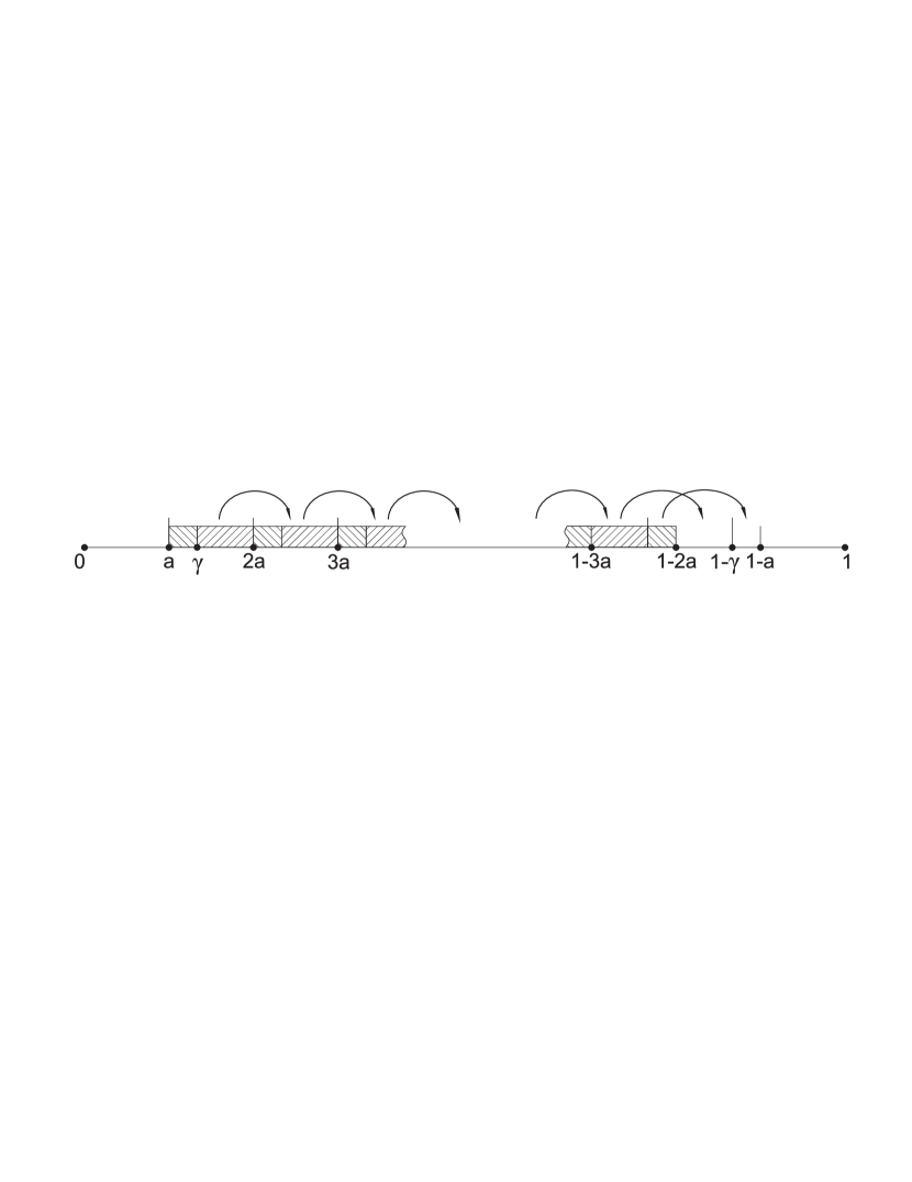
Figure 3: Scheme of induction in system (7)

Let $\frac{1}{n+1}<a\leq\frac{1}{n}$, $n=3,4,\ldots$ Note that $\gamma=1-(n-1)a$ ($n\leq\frac{1}{a}<n+1$, $\left[\frac{1}{a}\right]=n$, $\left[\frac{1-a}{a}\right]=\left[\frac{1}{a}\right]-1=n-1$) and $a\leq\gamma<2a$. We will use system (7) again. In order to improve visibility we will highlight interesting expression in a chain of inequalities in bold. Take $y_{0}\in[a,\gamma)$, then, for $m=n-2$,

$$a\leq(n-2)a=a+(n-3)a\leq\mathbf{y_{0}+(n-2)a-a}<1-(n-1)a+(n-3)a=1-2a.$$

On the other hand, whereas

$$1-2a<(n-1)a\leq\mathbf{y_{0}+(n-2)a}<1-a,$$

we can use the formula (8) and the third equality of system (7):

$$\frac{1}{1-a}\;p\!\left(\frac{y_{0}+(n-2)a}{1-a}\right)-p(y_{0}+(n-1)a)=A_{1}(y_{0}+(n-2)a)=\cr=\sum\limits_{k=-1}^{n-2}p(y_{0}+ka)-\frac{1}{1-a}\sum\limits_{k=-1}^{n-3}p\!\left(\frac{y_{0}+ka}{1-a}\right),$$

which implies formula (3).

Now take $y_{1}\in[\gamma,2a)$. If $n\geq 4$, then, for $m=n-3$,

$$a\leq 1-3a=\gamma+(n-3)a-a\leq\mathbf{y_{1}+(n-3)a-a}<2a+(n-3)a-a\leq 1-2a.$$

On the other hand, whereas

$$1-2a\leq\mathbf{y_{1}+(n-3)a}<1-a,$$

we can write:

$$\frac{1}{1-a}\;p\!\left(\frac{y_{1}+(n-3)a}{1-a}\right)-p(y_{1}+(n-2)a)=A_{1}(y_{1}+(n-3)a)=\cr=\sum\limits_{k=-1}^{n-3}p(y_{1}+ka)-\frac{1}{1-a}\sum\limits_{k=-1}^{n-4}p\!\left(\frac{y_{1}+ka}{1-a}\right),$$

which implies formula (4).

If $n=3$, then $y_{1}\in[a,2a)\cap[1-2a,1-a]$. Therefore, we get formula (4) by equating the first and the third equalities in the system (7).

2. Now let $\frac{1}{3}<a\leq\frac{1}{2}$. In this case $\frac{1-2a}{1-a}<\frac{a}{1-a}$ and formula (1) can be written in the following way:

$$\frac{p(x)}{1-a}=\begin{cases}p((1-a)x)+A_{2}((1-a)x+a),&x\in\left[\left.0,\frac{1-2a}{1-a}\right.\right);\\[5.69046pt] p((1-a)x)+p((1-a)x+a),&x\in\left[\left.\frac{1-2a}{1-a},\frac{a}{1-a}\right.\right);\\[5.69046pt] p((1-a)x+a)+A_{1}((1-a)x),&x\in\left[\frac{a}{1-a},1\right].\end{cases}$$ (9)

Consider the first equality of the system: $\frac{p(x)}{1-a}=p((1-a)x)+A_{2}((1-a)x+a)$, $x\in\left[\left.0,\frac{1-2a}{1-a}\right.\right)$. Make a change $y=(1-a)x+a$, then, for $y\in[a,1-a)$,

$$\frac{1}{1-a}\;p\!\left(\frac{y-a}{1-a}\right)=p(y-a)+A_{2}(y)=p(y-a)+p(y)-A_{1}(y).$$ (10)

Consider the second equality of the system: $\frac{p(x)}{1-a}=p((1-a)x)+p((1-a)x+a)$, $x\in\left[\left.\frac{1-2a}{1-a},\frac{a}{1-a}\right.\right)$. Make a change $y=(1-a)x+a$, then, for $y\in[1-a,2a)$,

$$\frac{1}{1-a}\;p\!\left(\frac{y-a}{1-a}\right)=p(y)+p(y-a).$$ (11)

Consider the third equality of the system: $\frac{p(x)}{1-a}=p((1-a)x+a)+A_{1}((1-a)x)$, $x\in\left[\frac{a}{1-a},1\right]$. Make a change $y=(1-a)x$, then, for $y\in[a,1-a]$,

$$A_{1}(y)=\frac{1}{1-a}\;p\!\left(\frac{y}{1-a}\right)-p(y+a).$$ (12)

Equating the values of $A_{1}(y)$ obtained from equations (10) and (12) for $y\in[a,1-a)$, and taking in account equation (11), we exactly get formulae (3)–(5) for $n=2$.

Conversely, $\mu_{S}=\mu$ provided that (3)–(5) hold true. Indeed, these conditions do not set a value of $\alpha_{1}(x)$ in the point $1-a$, but on the interval $[a,1-a)$ they are equivalent to the system (7) (for $n\geq 3$) or to conditions (10)–(12) (for $n=2$). Therefore almost everywhere (excluding point$x=1$ ($y=1-a$)) equality (1) holds true. ∎

For the sake of clarity we provide two Corollaries from the Theorem.

Given measure $\mu\ll\lambda$, there exists equipped $2$-transformation $S(a,\alpha)$ preserving measure $\mu$ if and only if parameters $p(x)$, $a$ and $\alpha=\{\alpha_{1}(x),\alpha_{2}(x)\}$ suffice the conditions (3)–(5).

Given equipped $2$-transformation $S(a,\alpha)$, there exists measure $\mu\ll\lambda$ which is preserved by $S$ if and only if the parameters $p(x)$, $a$ and $\alpha=\{\alpha_{1}(x),\alpha_{2}(x)\}$ suffice the conditions (3)–(5).

An example of trivial density is given in the following Theorem discussing the case of the Lebesgue measure ($\mu=\lambda$, $p\equiv 1$).

$\lambda_{S}=\lambda$ if and only if $a=\frac{1}{n}$, $n\in\mathbb{N}$, $n\geq 2$, and

$$\alpha_{1}(x)=\begin{cases}\frac{n-2}{n-1},&x\in\left[\left.\frac{1}{n},\frac{2}{n}\right.\right);\cr\frac{n-3}{n-1},&x\in\left[\left.\frac{2}{n},\frac{3}{n}\right.\right);\cr\hskip 8.25128pt\vdots\cr\frac{1}{n-1},&x\in\left[\left.\frac{n-2}{n},\frac{n-1}{n}\right.\right).\end{cases}$$

On the intervals $\left[0,\frac{1}{n}\right)$, $\left[\frac{n-1}{n},1\right]$ function $\alpha_{1}(x)$ is arbitrary.

      Proof. .

We apply Theorem 2 for $p(x)=1$. The condition (3) loses its meaning, because the interval turns into an empty set:

$$n+1=\frac{1}{1-a}n,\quad x_{0}\in[a,1-(n-1)a)=\left[\frac{1}{n+1},\frac{1}{n+1}\right)=\emptyset.$$

Condition (4),

$$n=\frac{1}{1-a}(n-1),\quad x_{1}\in[1-(n-1)a,2a)=\left[\frac{1}{n},\frac{2}{n}\right),$$

immediately implies $a=\frac{1}{n}$. Condition (5) for $m=\overline{0,n-3}$ yields the following formula:

$$\alpha_{1}\!\left(x+\frac{m}{n}\right)=m+2-\frac{m+1}{1-\frac{1}{n}}=\frac{n-m-2}{n-1},\quad x\in\left[\frac{1}{n},\frac{2}{n}\right).$$

For $m=n-2$ the Condition (5) loses its meaning, because $[(n-1)a,1-a)=\emptyset$. In particular for $n=2$ the equipment can be chosen arbitrarily.

Thus summing up aforesaid we obtain the formula

$$\alpha_{1}(x)=\frac{n-k}{n-1},\quad x\in\left[\frac{k-1}{n},\frac{k}{n}\right),\quad k=\overline{2,n-1},$$

which implies the statement of the Theorem. ∎

If $a=\frac{1}{2}$, then $\lambda_{S}=\lambda$ for every $\alpha$.

Corollary 2 agrees with a known result [1]: diadic transformation $S(x)=2x\ (\!\!\!\mod 1)$ preserves the Lebesgue measure.

However, our construction admits not only trivial density: equalities (3)–(5) are possible when $p(x)$ is not a constant.

For all $n=2,3,\ldots$ there exists parameter $a$, $\frac{1}{n+1}<a<\frac{1}{n}$, density $p(x)$ and equipment $\{\alpha_{1}(x),\alpha_{2}(x)\}$ such that $\mu_{S}=\mu$. Furthermore density $p(x)$ is not a constant.

      Proof. .

First consider the case of even $n=2m$. Let $a=\frac{2m+1-\sqrt{4m^{2}+1}}{2m}=\frac{n+1-\sqrt{n^{2}+1}}{n}$ be the root of the equation

$$\frac{ma}{1-a}=1-ma.$$ (13)

It is easy to verify that

$$\frac{1}{n+1}<a<\frac{1}{n}\qquad\left(\frac{1}{2m+1}<a<\frac{1}{2m}\right).$$ (14)

Let $\beta,\gamma\geq 0$. Consider a density given by the step function

$$p(x)=\beta\chi_{[0,ma)}(x)+(\beta+\gamma)(1-ma)\chi_{[ma,1-ma)}(x)+\gamma\chi_{[1-ma,1]}(x).$$

Let us show that it suffices the equalities (3)–(4). Thereto henceforward we will use conditions (13)–(14), and for better visibility will also highlight interesting parts of equalities in bold.

Consider condition (3). Let $x_{0}\in[a,1-(2m-1)a)$. For $-1\leq k\leq m-2$

$$0\leq\mathbf{\frac{x_{0}+ka}{1-a}}<\frac{1-(2m-1)a+ka}{1-a}\leq\frac{1-(m+1)a}{1-a}=ma.$$

For $m-1\leq k\leq n-2$

$$1-ma=\frac{ma}{1-a}\leq\frac{a+ka}{1-a}\leq\mathbf{\frac{x_{0}+ka}{1-a}}<1.$$

For $-1\leq k\leq m-2$

$$0\leq\mathbf{x_{0}+ka}<1-(2m-1)a+ka<(2m+1)a-(2m-1)a+ka=a(2+k)\leq ma.$$

For $k=m-1$

$$ma=(k+1)a\leq\mathbf{x_{0}+ka}<1-(2m-1)a+ka=1-ma.$$

For $m\leq k\leq n-1$

$$1-ma<(2m+1)a-ma=ma+a\leq a+ak\leq\mathbf{x_{0}+ka}<1.$$

In the case $\beta=\gamma=0$ equalities (3)–(4) are obviously fulfilled. Henceforth, we will assume $\beta+\gamma>0$. Then

$$\frac{\sum\limits_{k=-1}^{n-2}p\!\left(\frac{x_{0}+ka}{1-a}\right)}{\sum\limits_{k=-1}^{n-1}p(x_{0}+ka)}=\frac{m\beta+m\gamma}{m\beta+(\beta+\gamma)(1-ma)+m\gamma}=\frac{m}{1-ma+m}=1-a.$$

Consider condition (4). Let $x_{1}\in[1-(2m-1)a,2a)$. For $-1\leq k\leq m-3$

$$0<\mathbf{\frac{x_{1}+ka}{1-a}}<\frac{2a+ka}{1-a}\leq\frac{ma-a}{1-a}<ma.$$

For $k=m-2$

$$ma=\frac{1-(m+1)a}{1-a}=\frac{1-2ma+a+ka}{1-a}\leq\mathbf{\frac{x_{1}+ka}{1-a}}<\frac{2a+ka}{1-a}=\frac{ma}{1-a}=\\ =1-ma.$$

For $m-1\leq k\leq n-3$

$$1-ma<\frac{1-2ma+a+ma-a}{1-a}\leq\frac{1-(2m-1)a+ka}{1-a}\leq\mathbf{\frac{x_{1}+ka}{1-a}}<1.$$

For $-1\leq k\leq m-2$

$$0<\mathbf{x_{1}+ka}<2a+ka\leq ma.$$

For $m-1\leq k\leq n-2$

$$1-ma=1-(2m-1)a+ma-a\leq\mathbf{x_{1}+ka}<1.$$

Thus

$$\frac{\sum\limits_{k=-1}^{n-3}p\!\left(\frac{x_{1}+ka}{1-a}\right)}{\sum\limits_{k=-1}^{n-2}p(x_{1}+ka)}\!=\!\frac{(m-1)\beta+(\beta+\gamma)(1-ma)+(m-1)\gamma}{m\beta+m\gamma}\!=\!\frac{m(1-a)}{m}\!=\!1-a.$$

The case of odd $n=2m-1$, $m=2,3,\ldots$ we will describe in less detail. Let $a=\frac{m-\sqrt{m^{2}-m}}{m}=\frac{n+1-\sqrt{n^{2}-1}}{n+1}$ be the root of the equation

$$\frac{(m-1)a}{1-a}=1-ma\qquad\left(\frac{1}{n+1}<a<\frac{1}{n}\right).$$ (15)

Let $p(x)=\beta\chi_{[0,1-ma)}(x)+(\beta+\gamma)(1-ma)\chi_{[1-ma,ma)}(x)+\gamma\chi_{[ma,1]}(x)$, where $\beta,\gamma\geq 0$. Let us show that $p(x)$ suffices the equalities (3)–(4).

Consider condition (3). Let $x_{0}\in[a,1-(2m-2)a)$. Then

$$\hskip 9.3894pt\frac{x_{0}+ka}{1-a}\in\begin{cases}[0,1-ma),&-1\leq k\leq m-3;\cr[1-ma,ma),&k=m-2;\cr(ma,1),&m-1\leq k\leq n-2,\end{cases}$$

$$x_{0}+ka\in\begin{cases}[0,1-ma),&-1\leq k\leq m-2;\cr[ma,1),&m-1\leq k\leq n-1,\end{cases}$$

$$\frac{\sum\limits_{k=-1}^{n-2}p\!\left(\frac{x_{0}+ka}{1-a}\right)}{\sum\limits_{k=-1}^{n-1}p(x_{0}+ka)}\!=\!\frac{(m-1)\beta+(\beta+\gamma)(1-ma)+(m-1)\gamma}{m\beta+m\gamma}\!=\!\frac{m(1-a)}{m}\!=\!1-a.$$

Consider condition (4). Let $x_{1}\in[1-(2m-2)a,2a)$. Then

$$\frac{x_{1}+ka}{1-a}\in\begin{cases}(0,1-ma),&-1\leq k\leq m-3;\cr[ma,1),&m-2\leq k\leq n-3,\end{cases}\phantom{\ \;\,}$$

$$x_{1}+ka\in\begin{cases}(0,1-ma),&-1\leq k\leq m-3;\cr[1-ma,ma),&k=m-2;\cr(ma,1),&m-1\leq k\leq n-2,\end{cases}$$

$$\frac{\sum\limits_{k=-1}^{n-3}p\!\left(\frac{x_{1}+ka}{1-a}\right)}{\sum\limits_{k=-1}^{n-2}p(x_{1}+ka)}=\frac{(m-1)\beta+(m-1)\gamma}{(m-1)\beta+(\beta+\gamma)(1-ma)+(m-1)\gamma}=\frac{m-1}{m-ma}=1-a.$$

It remains to show that for the function $\alpha_{1}\!(x)$ given by the formula (5), $0\!\leq\!\alpha_{1}(x)\!\leq\!1$. We will find out $\alpha_{1}(x)$ explicitly.

Recall formula (5):

$$\alpha_{1}(x+sa)p(x+sa)=\sum\limits_{k=-1}^{s}p(x+ka)-\frac{1}{1-a}\sum\limits_{k=-1}^{s-1}p\!\left(\frac{x+ka}{1-a}\right),$$

where $x+sa\in\left\{\begin{array}[]{ll}[(s+1)a,(s+2)a)&\hbox{for }s=\overline{0,n-3};\cr[(s+1)a,1-a)&\hbox{for }s=n-2.\end{array}\right.$

To find $\alpha_{1}(x)$ we have to consider $10$ following cases. In doing this, we will use inequalities from above on numbers $x+ka$ and $\frac{x+ka}{1-a}$. In cases 1.1.1–2.2.3, when we divide by $\beta$, $\gamma$ or $\beta+\gamma$, we assume $\beta>0$, $\gamma>0$ or $\beta+\gamma>0$ correspondingly. Otherwise ($\beta=0$, $\gamma=0$ or $\beta+\gamma=0$) the values of $\alpha_{1}(x+sa)$ can be chosen arbitrarily ($\alpha_{1}(x)\in L^{1}$, $0\leq\alpha_{1}(x)\leq 1$).

1. $n=2m$. Note here that $\frac{ma}{1-a}=1-ma$.

1.1. $x\in[a,1-(n-1)a)$.

1.1.1. $0\leq s\leq m-2$, then

$$\alpha_{1}(x+sa)=\frac{1}{\beta}\left((s+2)\beta-\frac{1}{1-a}(s+1)\beta\right)=s+2-\frac{s+1}{1-a}.$$

1.1.2. $s=m-1$, then

$$\alpha_{1}(x+sa)=\\ =\frac{1}{(\beta+\gamma)(1-ma)}\left((s+1)\beta+(\beta+\gamma)(1-ma)-\frac{1}{1-a}(s+1)\beta\right)\!\!=\frac{\gamma}{\beta+\gamma}.$$ (16)

1.1.3. $m\leq s\leq n-2$, then

$$\alpha_{1}(x+sa)=\\ =\frac{1}{\gamma}\left(m\beta+(\beta+\gamma)(1-ma)+(s-m+1)\gamma-\frac{1}{1-a}(m\beta+(s-m+1)\gamma)\right)\!\!=\\ =\frac{1}{\gamma}\left((1-ma)\gamma+(s-m+1)\gamma-\frac{1}{1-a}(s-m+1)\gamma\right)=\\ =\frac{a(2m-s-1)}{1-a}.$$

1.2. $x\in[1-(n-1)a,2a)$.

1.2.1. $0\leq s\leq m-2$, then

$$\alpha_{1}(x+sa)=\frac{1}{\beta}\left((s+2)\beta-\frac{1}{1-a}(s+1)\beta\right)=s+2-\frac{s+1}{1-a}.$$

1.2.2. $m-1\leq s\leq n-3$, then

$$\alpha_{1}(x+sa)=\frac{1}{\gamma}\left(\hskip-25.6073pt\phantom{\frac{1}{1-a}}m\beta+(s-m+2)\gamma-\right.\\ \left.-\frac{1}{1-a}((m-1)\beta+(\beta+\gamma)(1-ma)+(s-m+1)\gamma)\right)=\\ =\frac{a(2m-s-2)}{1-a}.$$

2. $n=2m-1$. Note here that $\frac{(m-1)a}{1-a}=1-ma$.

2.1. $x\in[a,1-(2m-2)a)$.

2.1.1. $0\leq s\leq m-2$, then

$$\alpha_{1}(x+sa)=\frac{1}{\beta}\left((s+2)\beta-\frac{1}{1-a}(s+1)\beta\right)=s+2-\frac{s+1}{1-a}.$$

2.1.2. $m-1\leq s\leq n-2$, then

$$\alpha_{1}(x+sa)=\frac{1}{\gamma}\left(m\beta+(s-m+2)\gamma-\phantom{\frac{1}{1-a}}\right.\\ \left.-\frac{1}{1-a}((m-1)\beta+(\beta+\gamma)(1-ma)+(s-m+1)\gamma\right)=\frac{a(2m-s-2)}{1-a}.$$

2.2. $x\in[1-(2m-2)a,2a)$.

2.2.1. $0\leq s\leq m-3$, then

$$\alpha_{1}(x+sa)=\frac{1}{\beta}\left((s+2)\beta-\frac{1}{1-a}(s+1)\beta\right)=s+2+\frac{s+1}{1-a}.$$

2.2.2. $s=m-2$, then

$$\alpha_{1}(x+sa)=\\ =\frac{1}{(\beta+\gamma)(1-ma)}\left((s+1)\beta+(\beta+\gamma)(1-ma)-\frac{1}{1-a}(s+1)\beta\right)=\frac{\gamma}{\beta+\gamma}.$$

2.2.3. $m-1\leq s\leq n-3$, then

$$\alpha_{1}(x+sa)=\frac{1}{\gamma}\left((m-1)\beta+(\beta+\gamma)(1-ma)+(s-m+2)\gamma-\phantom{\frac{1}{1-a}}\right.\\ \left.-\frac{1}{1-a}((m-1)\beta+(s-m+2)\gamma)\right)=\frac{a(2m-s-3)}{1-a}.$$

We sum up formulae for $\alpha_{1}(x)$ obtained above in more compact way.

For $n=2m$, $x\in[a,1-(n-1)a)$,

$$\alpha_{1}(x+sa)=\left\{\begin{array}[]{ll}s+2-\frac{s+1}{1-a},&0\leq s\leq m-2;\\ \frac{\gamma}{\beta+\gamma},&s=m-1;\\ \frac{a(n-s-1)}{1-a},&m\leq s\leq n-2.\phantom{\hskip 14.22636pt}\end{array}\right.$$

For $n=2m$, $x\in[1-(n-1)a,2a)$,

$$\alpha_{1}(x+sa)=\left\{\begin{array}[]{ll}s+2-\frac{s+1}{1-a},&0\leq s\leq m-2;\\ \frac{a(n-s-2)}{1-a},&m-1\leq s\leq n-3.\end{array}\right.$$

For $n=2m-1$, $x\in[a,1-(n-1)a)$,

$$\alpha_{1}(x+sa)=\left\{\begin{array}[]{ll}s+2-\frac{s+1}{1-a},&0\leq s\leq m-2;\\ \frac{a(n-s-1)}{1-a},&m-1\leq s\leq n-2.\end{array}\right.$$

For $n=2m-1$, $x\in[1-(n-1)a,2a)$,

$$\alpha_{1}(x+sa)=\left\{\begin{array}[]{ll}s+2-\frac{s+1}{1-a},&0\leq s\leq m-3;\\ \frac{\gamma}{\beta+\gamma},&s=m-2;\\ \frac{a(n-s-2)}{1-a},&m-1\leq s\leq n-3.\end{array}\right.$$

Thus $0<\alpha_{1}(x)<1$, since for $k=1,2$

$$0<\frac{1-ma}{1-a}\leq\mathbf{s+2-\frac{s+1}{1-a}}=\frac{1-2a-sa}{1-a}\leq\frac{1-2a}{1-a}<1,\quad 0\leq s\leq m-2,$$

$$0<\frac{a}{1-a}\leq\mathbf{\frac{a(n-s-k)}{1-a}}\leq\frac{am}{1-a}<1,\quad m-1\leq s\leq n-3.$$

Using Theorem 2 for an equipment $\alpha$ given by the formula (5) we obtain $\mu_{S}=\mu$. ∎

In the proof of Theorem 2 we have actually found a family of densities depending on two parameters $\beta,\gamma\geq 0$.

As an example we provide the plots of density $p(x)$ and weight function $\alpha_{1}(x)$ for the case of $n=10$, see fig. 4. We used $\beta=1$, $\gamma=2$, $\alpha_{1}(x)=\cos x$ for $x\in[0,a)$, $\alpha_{1}(x)=\sin x$ for $x\in[1-a,1]$.

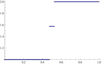
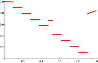
Figure 4: Density $p(x)$ plot (to the left) and weight function $\alpha_{1}(x)$ plot (to the right), here $n=10$

For all $\beta,\gamma\geq 0$ chosen in the proof of Theorem 2,

$$\mu([0,1])=\left\{\begin{array}[]{ll}\left(1+n^{2}-n\sqrt{n^{2}+1}\right)(\beta+\gamma),&n\hbox{ is even;}\\ \left(1-n^{2}+n\sqrt{n^{2}-1}\right)(\beta+\gamma),&n\hbox{ is odd.}\end{array}\right.$$

In particular we can chose $\beta+\gamma$ such that $\mu([0,1])=1$.

      Proof. .

If $n=2m$, then $ma=(n+1-\sqrt{n^{2}+1})/2$ (see formula (13)) and

$$\!\!\!\mu([0,1])=\int_{0}^{1}\!\left(\beta\chi_{[0,ma)}(x)+(\beta+\gamma)(1-ma)\chi_{[ma,1-ma)}(x)+\gamma\chi_{[1-ma,1]}(x)\right)d\lambda=\\ =\left(ma+(1-ma)(1-2ma)\right)(\beta+\gamma)=\left(1+n^{2}-n\sqrt{n^{2}+1}\right)(\beta+\gamma).$$

If $n=2m-1$, then $ma=(n+1-\sqrt{n^{2}-1})/2$ (see formula (15)) and

$$\!\!\!\mu([0,1])=\int_{0}^{1}\!\left(\beta\chi_{[0,1-ma)}(x)+(\beta+\gamma)(1-ma)\chi_{[1-ma,ma)}(x)+\gamma\chi_{[ma,1]}(x)\right)d\lambda=\\ =\left(2ma(1-ma)\right)(\beta+\gamma)=\left(1-n^{2}+n\sqrt{n^{2}-1}\right)(\beta+\gamma).$$

∎

As a conclusion let us consider the following. Let $n=2$. By Theorem 2 for the number $a=\frac{3-\sqrt{5}}{2}\in\left(\frac{1}{3},\frac{1}{2}\right]$ and density $p(x)=\beta\chi_{[0,a)}(x)+\beta(1-a)\chi_{[a,1-a)}(x)$ (we use $\gamma=0$) $\mu_{S}=\mu$. Condition (5) turns to the following:

$$\alpha_{1}(x)p(x)=p(x-a)+p(x)-\frac{1}{1-a}\;p\!\left(\frac{x-a}{1-a}\right),\quad x\in[a,1-a).$$

Then $x-a\in[0,1-2a)\subset[0,a)$, $\frac{x-a}{1-a}\in\left[0,\frac{1-2a}{1-a}\right)=[0,a)$ and we obtain

$$\alpha_{1}(x)\beta=\frac{1}{1-a}\left(\beta+\beta(1-a)-\frac{1}{1-a}\beta\right)=0$$

(this result also follows from formula (16) given in the proof of Theorem 2).

Let us take $\alpha_{1}(x)\equiv 0$, $\alpha_{2}(x)\equiv 1$. This case corresponds to single-valued dynamical system $([0,1],\mathfrak{B},\mu,S_{2})$ consisting of one function $S_{2}$. The support of a measure of such system lays inside $[0,1-a]$. Being restricted to $[0,1-a]$, transformation $S_{2}$ coincides with the mapping

$$Tx=\frac{1}{1-a}x\quad(\!\!\!\!\!\mod 1-a),$$

acting by the rule $Tx=(1-a)\left\{\frac{1}{(1-a)^{2}}x\right\}$. Note that $\frac{1}{1-a}=\frac{\sqrt{5}+1}{2}$ is a <<golden ratio>> (being also a <<simple $\beta$-number>>, see [2]). On the fig. 5 we depict the plot of transformation $S_{2}$ in the square $[0,1]\times[0,1]$ and the plot of mapping $T$ in the smaller square $[0,1-a]\times[0,1-a]$.

Figure 5: Scheme of transformations $S_{2}$ and $Tx=\frac{1}{1-a}x(\!\!\!\mod 1-a)$                           (in the small square region)

Let us normalize the density $p(x)$ such that $\mu([0,1-a])=1-a$:

$$\mu([0,1-a])=\int_{0}^{1-a}p(x)\,d\lambda=\beta a+\beta(1-a)(1-2a)=1-a,$$

whence $\beta=\frac{5+3\sqrt{5}}{10}$, $\beta(1-a)=\frac{5+\sqrt{5}}{10}$. For the sake of simplicity we let also $p(1-a)=\frac{5+\sqrt{5}}{10}$ (since p$(x)$ is defined $\lambda$-almost everywhere).

Thus we get invariant measure for the dynamical system $([0,1-a],\mathfrak{B}^{\prime},\mu^{\prime},T)$ (here $\mathfrak{B}^{\prime}$ is a $\sigma$-field obtained by intersecting sets from $\mathfrak{B}$ with the segment $[0,1-a]$, $\mu^{\prime}=\mu_{|_{\mathfrak{B}^{\prime}}}$).

Transformation $S_{2}|_{[0,1-a]}(x)=Tx\colon[0,1-a]\to[0,1-a]$ preserves measure $\mu^{\prime}(\tilde{p})$ with density

$$\tilde{p}(x)=\left\{\begin{array}[]{ll}\frac{5+3\sqrt{5}}{10},&0\leq x<\frac{3-\sqrt{5}}{2};\\ \frac{5+\sqrt{5}}{10},&\frac{3-\sqrt{5}}{2}\leq x\leq\frac{\sqrt{5}-1}{2}\hbox{.}\end{array}\right.$$

This agrees with classical result (adapted for the segment $[0,1-a]$) obtained by A. Rényi in [1] (see also [2]): transformation $T$ is ergodic and has a unique invariant measure (with density $\tilde{p}(x)$) equivalent to the Lebesgue measure.

References

[1]A. Rényi, ‘‘Representations for real numbers and their
ergodic properties,’’
Acta Math. Acad. Sci. Hung., vol. 8, pp. 477–493, 1957.
[2]W. Parry, ‘‘On the -expansions of real numbers,’’ Acta Math. Acad.
Sci. Hung., vol. 11, pp. 401–416, 1960.
[3]N. Sidorov, ‘‘Arithmetic dynamics,’’ in Topics in
dynamics and ergodic
theory (S. Bezuglyi and S. F. Kolyada, eds.), vol. 310 of London
Mathematical Society lecture note series, pp. 145–189, Cambridge University
Press, 2003.
[4]P. Erdős, I. Joó, and V. Komornik, ‘‘Characterization of
the unique
expansions and related problems,’’ Bull.
Soc. Math. France, vol. 118, pp. 377–390, 1990.
[5]N. Sidorov, ‘‘Almost every number has a continuum of
-expansions,’’ Amer. Math. Monthly, vol. 110, pp. 838–842, 2003.
[6]N. Sidorov, ‘‘Expansions in non-integer bases: Lower, middle
and top orders,’’
J. Number Theory, vol. 129, no. 4, pp. 741–754, 2009.
[7]К. Б. Игудесман, ‘‘Верхние адреса для одного семейства систем
итерированных
функций на отрезке,’’ Известия вузов. Математика, vol. 9, pp. 75–81,
2009. (in Russian, but also available in English in Russian Mathematics (Iz. VUZ), vol. 53, no. 9, pp. 67–72, 2009.)
[8]А. О. Гельфонд, ‘‘Об одном общем свойстве систем счисления,’’
Известия
академии наук СССР. Серия математическая, vol. 23, pp. 809–814, 1959.
[9]M. F. Barnsley, ‘‘Theory and application of fractal tops,’’ in
Fractals in
engineering: new trends in theory and applications (J. Lévy-Véhel and
E. Lutton, eds.), pp. 3–20, Springer-Verlag, London Limited, 2005.
[10]P. Erdős, ‘‘On a family of symmetric Bernoulli
convolutions,’’ Amer.
J. Math., vol. 61, pp. 974–975, 1939.
[11]Y. Peres, W. Schlag, and B. Solomyak, ‘‘Sixty years of
Bernoulli
convolutions,’’ in Fractal Geometry and Stochastics II (C. Bandt,
S. Graf, and M. Zaehle, eds.), vol. 46 of Progress in probability,
pp. 39–65, Birkhauser, 2000.
[12]P. I. Troshin, ‘‘Multivalued dynamic systems with weights,’’
Izvestiya Vysshikh Uchebnykh Zavedenii. Matematika, vol. 7,
pp. 35–50, 2009. (in Russian, but also available in English in Russian Mathematics (Iz. VUZ), vol. 53, no. 7, pp. 28–42, 2009.)Paul I. Troshin – chair of Geometry of Kazan State
University, Kazan, Russia
E-mail: Paul.Troshin@gmail.com