On the efficient computation of high-order derivatives for implicitly defined functions

Abstract

Scientific studies often require the precise calculation of derivatives. In many cases an analytical calculation is not feasible and one resorts to evaluating derivatives numerically. These are error-prone, especially for higher-order derivatives. A technique based on algorithmic differentiation is presented which allows for a precise calculation of higher-order derivatives. The method can be widely applied even for the case of only numerically solvable, implicit dependencies which totally hamper a semi-analytical calculation of the derivatives. As a demonstration the method is applied to a quantum field theoretical physical model. The results are compared with standard numerical derivative methods.

1 Physical motivation

In many scientific studies the knowledge of derivatives of a given quantity is of particular importance. For example in theoretical physics, especially in thermodynamics, many quantities of interest require the calculation of derivatives of an underlying thermodynamic potential with respect to some external parameters such as temperature, volume, or chemical potentials. In many cases the thermodynamic potentials can only be evaluated numerically and one is forced to employ numerical differentiation techniques which are error-prone as any numerical methods. Furthermore, the thermodynamic potential has to be evaluated at the physical point defined by minimizing the thermodynamic potential with respect to some condensates yielding the equations of motion (EoM). Generally, these equations can be solved only numerically and thus introduce additional implicit dependencies which makes the derivative calculations even more complicated.

Even in cases where the thermodynamic potential and the implicit dependencies on the external parameters are known analytically, the evaluation of higher-order derivatives becomes very complex and tedious and in the end impedes their explicit calculation.

In this work we present a novel numerical technique, based on algorithmic differentiation (AD) to evaluate derivatives of arbitrary order of a given quantity at machine precision. Compared to other differentiation techniques such as the standard divided differentiation (DD) method or symbolic differentiation, the AD produces truncation-error-free derivatives of a function which is coded in a computer program. Additionally, AD is fast and reduces the work required for analytical calculations and coding, especially for higher-order derivatives. Furthermore, the AD technique is applicable even if the implicit dependencies on the external parameters are known only numerically. In Ref. [1] a comprehensive introduction to AD can be found. First remarks about the computation of derivative of implicitly defined functions were already contained in [2]. However, a detailed description and analysis is not available yet. Additional information about tools and literature on AD are available on the web-page of the AD-community [3].

This work is organized in the following way: For illustrations we will introduce an effective model, the so-called linear sigma model with quark degrees of freedom in Sec. 2. This model is widely used for the description of the low-energy sector of strongly interacting matter. As a starting point the basic thermodynamic grand potential and the EoM of this model are calculated in a simple mean-field approximation in order to elucidate the technical problems common in such types of calculations. Before we demonstrate the power of the AD method by calculating certain Taylor expansion coefficients up to very high orders for the first time in Sec. 6, the AD method itself and some mathematical details are introduced in Sec. 3. Details for the calculation of higher-order derivatives of implicit functions are given in the following Sec. 4. In Sec. 5 the results of the AD method are confronted with the ones of the standard divided differences (DD) method in order to estimate the truncation and round off errors. Finally, we end with a summary and conclusion in Sec. 7.

2 A model example

In order to illustrate the key points of the AD method we employ a quantum field theoretical model [4]. This model can be used to investigate the phase structure of strongly interacting matter described by the underlying theory of Quantum Chromodynamics (QCD). Details concerning this effective linear sigma model (L$\sigma$M) in the QCD context can be found in reviews, see e.g. [5, 6].

The quantity of interest for the exploration of the phase structure is the grand potential of the L$\sigma$M. This thermodynamic potential depends on the temperature $T$ and quark chemical potential $\mu$ because the particle number can also vary. It is calculated in mean-field approximation whose derivation for three quark flavors is shown explicitly in [7]. For the L$\sigma$M the total grand potential $\Omega$ consists of two contributions

$$\Omega(T,\mu;\sigma_{q},\sigma_{s})=U\left(\sigma_{q},\sigma_{s}\right)+\Omega_{\bar{q}q}(T,\mu;\sigma_{q},\sigma_{s})\ ,$$ (1)

where the first part, $U$, stands for the purely mesonic potential contribution and is a function of two condensates, $\sigma_{q}$ and $\sigma_{s}$. The second part, $\Omega_{\bar{q}q}$, is the quark contribution and depends on the two condensates as well as on the external parameters temperature $T$ and, for simplicity, only one quark chemical potential $\mu$. Since the quark contribution arises from a momentum-loop integration over the quark fields, it is given by an integral which cannot be evaluated in closed form analytically. Readers who are unfamiliar with the physical details, may simply regard Eq. (1) as an only numerically known function and continue with the reading above Eq. (6), which introduces an implicit dependency on the parameters $T$ and $\mu$ whose treatment with the AD technique is the major focus of this work.

Explicitly, in mean-field approximation the quark contribution reads

$$\Omega_{\bar{q}q}=6T\sum_{f=u,d,s}\int\limits_{0}^{\infty}\!\frac{d^{3}k}{(2\pi)^{3}}\left\{\ln\left(1-n_{q,f}(T,\mu)\right)\right.\\ +\left.\ln(1-{\bar{n}}_{\bar{q},f}(T,\mu))\right\}\ ,$$ (2)

where a summation over three quark flavors $f$ is included. The usual fermionic occupation numbers for the quarks are denoted by

$$n_{q,f}(T,\mu)=\frac{1}{1+\exp\left((E_{q,f}-\mu)/T\right)}$$ (3)

and for antiquarks by ${\bar{n}}_{\bar{q},f}(T,\mu)\equiv n_{q,f}(T,-\mu)$ respectively. In this example only two different single-particle energies, $E_{q,i},\ i=q,s$, emerge

$$E_{q,q}=\sqrt{k^{2}+(g\sigma_{q}/2)^{2}}\quad\text{and}\quad E_{q,s}=\sqrt{k^{2}+(g\sigma_{s}/\sqrt{2})^{2}}\ .$$ (4)

The first index $i=q$ denotes the combination of two mass-degenerate light-quark flavors ($u,d$) and the other index $s$ labels the heavier strange quark flavor. The expressions in parentheses in $E_{q,i}$ are the corresponding quark masses. In this way, the dependency of the grand potential on the condensates, $\sigma_{i}$, $i=q,s$ enter through the quark masses, which has not been indicated explicitly in Eq. (2).

The mesonic potential does not depend on the quark chemical potential nor on the temperature explicitly. It is just a function of the two condensates and reads

$$U(\sigma_{q},\sigma_{s})=\frac{m^{2}}{2}\left(\sigma_{q}^{2}+\sigma_{s}^{2}\right)-h_{q}\sigma_{q}-h_{s}\sigma_{s}-\frac{c}{2\sqrt{2}}\sigma_{q}^{2}\sigma_{s}\\ +\frac{\lambda_{1}}{2}\sigma_{q}^{2}\sigma_{s}^{2}+\frac{1}{8}\left(2\lambda_{1}+\lambda_{2}\right)\sigma_{q}^{4}+\frac{1}{8}\left(2\lambda_{1}+2\lambda_{2}\right)\sigma_{s}^{4}\ ,$$ (5)

wherein all remaining quantities, e.g. $m,h_{q},\ldots$ are constant parameters.

Since the physical condensates, $\bar{\sigma}_{q}$ and $\bar{\sigma}_{s}$, are determined by the extrema (minima) of the total grand potential with respect to the corresponding fields, they fulfill the equations of motion

$$\left.\frac{\partial\Omega(T,\mu;\sigma_{q},\sigma_{s}))}{\partial\sigma_{i}}\right|_{\scriptsize\begin{array}[]{l}\sigma_{q}=\bar{\sigma}_{q},\\ \sigma_{s}=\bar{\sigma}_{s}\end{array}}=0\ ;\qquad i=q,s\ .$$ (6)

This in turn introduces an implicit $T$- and $\mu$-dependence of both condensates,

$$\bar{\sigma}_{i}=\bar{\sigma}_{i}(T,\mu)\ ;\qquad i=q,s\ .$$ (7)

These quantities represent the physical order parameters which, together with the grand potential, are the basis of the exploration of the phase structure of the model. We denote the grand potential evaluated at $\sigma_{i}=\bar{\sigma}_{i},$ $i=q,s$, as

$$\bar{\Omega}(T,\mu)=\Omega\left(T,\mu;\bar{\sigma}_{q}(T,\mu),\bar{\sigma}_{s}(T,\mu)\right)$$ (8)

In order to find the temperature and chemical potential behavior of the order parameters the integral in Eq. (2) and simultaneously the EoM have to be solved numerically. This already is an example suitable for an AD application, because a derivative of a only numerically solvable, implicit function is needed as input. Later we will be interested in higher-order derivatives of the grand potential with respect to, e.g., the chemical potential. For example, the quark number density at the physical point is defined by

$$\rho_{q}(T,\mu)=-\frac{\partial\bar{\Omega}(T,\mu)}{\partial\mu}\ .$$ (9)

In cases without an implicit $T$- or $\mu$-dependence in the thermodynamic potential some progress can be made by calculating the corresponding derivatives explicitly and solving the corresponding equations numerically. This might be feasible for lower-order derivatives, in particular, if parts of the derivative calculations can be performed by some computer algebra packages like Mathematica or Maple. But for higher-order derivatives this procedure is error-prone and time-consuming and not applicable anymore.

In the following sections the algorithmic differentiation technique for implicitly defined functions is introduced on a general mathematical level.

3 Algorithmic Differentiation

Suppose the function ${\bf F}:{\mathbb{R}}^{n}\mapsto{\mathbb{R}}^{m}$, ${\bf y}={\bf F}({\bf x})$ describing an arbitrary algebraic mapping from ${\mathbb{R}}^{n}$ to ${\mathbb{R}}^{m}$ is defined by an evaluation procedure in a high-level computer language like Fortran or C. The technique of algorithmic differentiation provides derivative information of arbitrary order for the code segment in the computer that evaluates ${\bf F}({\bf x})$ within working accuracy. For this purpose, the basic differentiation rules such as, e.g., the product rule are applied to each statement of the given code segment. This local derivative information is then combined by the chain rule to calculate the overall derivatives. Hence the code is decomposed into a long sequence of simple evaluations, e.g., additions, multiplications, and calls to elementary functions such as $\sin(x)$ or $\exp(x)$, the derivatives of which can be easily calculated. Exploiting the chain rule yields the derivatives of the whole sequence of statements with respect to the input variables.

As an example, consider the function ${\bf F}:{\mathbb{R}}^{3}\rightarrow{\mathbb{R}}^{2}$ with

$$y_{1} =\sin(x_{1}*x_{2})$$

$$y_{2} =x_{3}+\cos(x_{1}*x_{2})$$

that can be evaluated by the pseudo-code given on the left column of Tab. 1. On the right-hand side, the resulting statements for the derivative calculation $\dot{\bf y}={\bf F}^{\prime}({\bf x})\dot{\bf x}$ are given.

$$\begin{array}[]{ll}v_{1}=x_{1}*x_{2}\phantom{XXXX}&\dot{v}_{1}=\dot{x}_{1}*x_{2}+x_{1}*\dot{x}_{2}\\ v_{2}=\sin(v_{1})&\dot{v}_{2}=\cos(v_{1})*\dot{v}_{1}\\ v_{3}=\cos(v_{1})&\dot{v}_{3}=-\sin(v_{1})*\dot{v}_{1}\\ v_{4}=x_{3}+v_{3}&\dot{v}_{4}=\dot{x}_{3}+\dot{v}_{3}\\ y_{1}=v_{2}&\dot{y}_{1}=\dot{v}_{2}\\ y_{2}=v_{4}&\dot{y}_{2}=\dot{v}_{4}\end{array}$$

Table 1: Function and derivative calculation.

For the vector $\dot{\bf x}=(1,0,0)^{T}$ one obtains the first column of the Jacobian $\nabla{\bf F}({\bf x})$ the vector $\dot{\bf y}=(\cos(x_{1}*x_{2})*x_{2}$, $-\sin(x_{1}*x_{2})*x_{2})^{T}$. Correspondingly, the other unit vectors in ${\mathbb{R}}^{3}$ yield the other two remaining columns of the Jacobian ${\bf F}^{\prime}({\bf x})$.

Table 1 illustrates the so-called forward mode of AD, where the derivatives are propagated together with the function evaluation. Alternatively, one may propagate the derivative information from the dependents ${\bf y}$ to the independents ${\bf x}$ yielding the so-called reverse mode of AD.

Over the past decades, extensive research activities led to a thorough understanding and analysis of these two basic modes of AD, where the complexity results with respect to the required runtime are based on the operation count $O_{\bf F}$, i.e., the number of floating point operations required to evaluate ${\bf F}({\bf x})$, and the degree $d$ of the computed derivatives. Using the forward mode, one computes the required derivatives together with the function evaluation in one sweep as illustrated above. The forward mode yields one column of the Jacobian $\nabla{\bf F}$ at no more than three times $O_{\bf F}$  [1]. One row of $\nabla{\bf F}$, e.g., the gradient of a scalar-valued component function of ${\bf F}$, is obtained using the reverse mode in its basic form also at no more than four times $O_{\bf F}$ [1]. It is important to note that this bound for the reverse mode is completely independent of the number $n$ of input variables. This observation is called cheap gradient result.

For the application discussed in the present work, the forward mode has been chosen for the efficient computation of higher-order derivatives which is illustrated in the following paragraphs. To this end, we consider Taylor polynomials of the form

$${\bf x}(t)\equiv \sum_{j=0}^{d}{\bf x}_{j}\,t^{j}\;:\;{\mathbb{R}}\;\mapsto\;{\mathbb{R}}^{n}$$

where (10)

$$\qquad{\bf x}_{j} =\frac{1}{j!}\left.\frac{\partial^{j}}{\partial t^{j}}{\bf x}(t)\;\right|_{t=0}$$

are scaled derivatives at $t=0$. The expansion is truncated at the highest derivative degree $d$ which is chosen by the user. The vector polynomial ${\bf x}(t)$ describes a path in ${\mathbb{R}}^{n}$ which is parameterized by $t$. Thus, the first two vectors $\bf x_{1}$ and $\bf x_{2}$ represent the tangent and the curvature at the base point ${\bf x}_{0}={\bf x}(0)$. Assuming that the function ${\bf y}={\bf F}({\bf x})$ is sufficiently smooth, i.e., $d$ times continuously differentiable, one obtains a corresponding value path

$${\bf y}(t) \equiv\sum_{j=0}^{d}{\bf y}_{j}\,t^{j}={\bf F}({\bf x}(t))+O(t^{d+1})\in{\mathbb{R}}^{m}.$$ (11)

The coefficient functions ${\bf y}_{j}$ are uniquely and smoothly determined by the coefficient vectors ${\bf x}_{i}$ with $i\leq j$. To compute this higher-order information, first we will examine for a given Taylor polynomial

$${\bf x}(t) ={\bf x}_{0}+{\bf x}_{1}\,t+{\bf x}_{2}\,t^{2}+\dots+{\bf x}_{d}\,t^{d}\in{\mathbb{R}}^{n}$$

the derivative computation based on “symbolic” differentiation.

Let us generalize the previous relation ${\bf y}(t)={\bf F}({\bf x}(t))$ given in Eq. (11), and consider now a general smooth function ${\bf v}(t)={\boldsymbol{\varphi}}({\bf x}(t))$ as for example the evaluation of a $\sin(.)$-function. This function ${\bf v}(t)$ represents one of the intermediate values computed during the function evaluation as illustrated in Table 1. One obtains for the Taylor coefficients

$${\bf v}_{j}=\frac{1}{j!}\left.\frac{\partial^{j}}{\partial t^{j}}{\bf v}(t)\;\right|_{t=0}\qquad\mbox{ and }\qquad{\bf{\boldsymbol{\varphi}}}_{j}(.)=\frac{1}{j!}{\boldsymbol{\varphi}}^{(j)}(.)$$

the derivative expressions

$${\bf v}_{0} ={\boldsymbol{\varphi}}({\bf x}_{0})$$

$${\bf v}_{1} ={\boldsymbol{\varphi}}{{}_{1}}({\bf x}_{0})\,{\bf x}_{1}$$

$${\bf v}_{2} ={\boldsymbol{\varphi}}{{}_{2}}({\bf x}_{0})\,{\bf x}_{1}\,{\bf x}_{1}+{\boldsymbol{\varphi}}{{}_{1}}({\bf x}_{0})\,{\bf x}_{2}$$

$${\bf v}_{3} ={\boldsymbol{\varphi}}{{}_{3}}({\bf x}_{0})\,{\bf x}_{1}\,{\bf x}_{1}\,{\bf x}_{1}+2\,{\boldsymbol{\varphi}}{{}_{2}}({\bf x}_{0})\,{\bf x}_{1}\,{\bf x}_{2}+{\boldsymbol{\varphi}}{{}_{1}}({\bf x}_{0})\,{\bf x}_{3}$$

$${\bf v}_{4} ={\boldsymbol{\varphi}}{{}_{4}}({\bf x}_{0})\,{\bf x}_{1}\,{\bf x}_{1}\,{\bf x}_{1}\,{\bf x}_{1}+3{\boldsymbol{\varphi}}{{}_{3}}({\bf x}_{0})\,{\bf x}_{1}\,{\bf x}_{1}\,{\bf x}_{2}$$

$$\phantom{=}+{\boldsymbol{\varphi}}{{}_{2}}({\bf x}_{0})\,({\bf x}_{2}\,{\bf x}_{2}+2\,{\bf x}_{1}\,{\bf x}_{3})+\,{\boldsymbol{\varphi}}{{}_{1}}({\bf x}_{0})\,{\bf x}_{4}$$

$$\phantom{=}\vdots$$

Hence, the overall complexity grows rapidly with the degree $d$ of the Taylor polynomial. To avoid these prohibitively expensive calculations the standard higher-order forward sweep of algorithmic differentiation is based on Taylor arithmetic [8] yielding an effort that grows like $d^{2}$ times the cost of evaluating ${\boldsymbol{\varphi}}({\bf x})$. This is quite obvious for arithmetic operations such as multiplications or additions, where one obtains the recursion shown in Table 2,

$v(t)=$	Formula $(1\leq k\leq d)$	OPS	MOVES
$x(t)+y(t)\;$	$\quad v_{k}=x_{k}+y_{k}$	$\sim 2d$	$3d$
$x(t)*y(t)\;$	$\quad v_{k}=\sum\limits_{j=0}^{k}x_{j}*y_{k-j}$	$\sim d^{2}$	$3d$

Table 2: Taylor coefficient propagation for arithmetic operations

where OPS denotes the total number of floating point operations and MOVES the total number of memory accesses required to compute all Taylor coefficients $v_{0},\ldots,v_{d}$. For a general elemental function $\varphi$, one finds also a recursion with quadratic complexity by interpreting $\varphi$ as solution of a linear ordinary differential equation as described in [1]. Table 3 illustrates the resulting computation of the Taylor coefficients for the exponential function

$v(t)=$	Formula $(1\leq k\leq d)$	OPS	MOVES
$\exp(x(t))$	$\quad kv_{k}=\sum\limits_{j=1}^{k}jv_{k-j}x_{j}$	$\sim d^{2}$	$2d$

Table 3: Taylor coefficient propagation for exponential

Similar formulas can be found for all intrinsic functions. This fact permits the computation of higher-order derivatives for the vector function ${\bf F}({\bf x})$ as composition of elementary components.

The AD-tool ADOL-C [9] uses the Taylor arithmetic as described above to provide an efficient calculation of higher-order derivatives.

4 Higher-order Derivatives of Implicit Functions

4.1 Basic Algorithm

For the application considered here, higher-order derivatives of a variable ${\bf y}\in{\mathbb{R}}^{m}$ are required, where ${\bf y}$ is implicitly defined as a function of some variable ${\bf x}\in{\mathbb{R}}^{n-m}$ by an algebraic system of equations

$${\bf G}({\bf z})\;=\;0\in{\mathbb{R}}^{m}\quad{\rm with}\quad{\bf z}=({\bf y},{\bf x})\in{\mathbb{R}}^{n}.$$

Naturally, the $n$ arguments of ${\bf G}$ need not be partitioned in this regular fashion. To provide flexibility for a convenient selection of the $p\equiv n-m$ truly independent variables $\bf x$, let ${\bf P}\in{\mathbb{R}}^{p\times n}$ be a projection matrix with only $0$ or $1$ entries that picks out these independent variables. Hence, ${\bf P}$ is a column permutation of the matrix $[0,{\bf I}_{p}]\in{\mathbb{R}}^{p\times n}$. Then the nonlinear system

$${\bf G}({\bf z})\;=\;0,\quad{\bf Pz}={\bf x},$$

has a regular Jacobian, wherever the implicit function theorem yields ${\bf y}$ as a function of ${\bf x}$. Therefore, we may also write with ${\bf H}:{\mathbb{R}}^{n}\mapsto{\mathbb{R}}^{n}$

$${\bf H}({\bf z})\equiv\left(\begin{array}[]{c}{\bf G}({\bf z})\\ {\bf P}{\bf z}\end{array}\right)\;=\;\left(\begin{array}[]{c}0\\ {\bf Pz}\end{array}\right)\;=\;{\bf S\,x},$$ (16)

for the seed matrix ${\bf S}=[0,{\bf I}_{p}]^{\top}\in{\mathbb{R}}^{n\times p}$. Now, we have rewritten the original implicit functional relation between ${\bf x}$ and ${\bf z}$ as an inverse relation ${\bf H}({\bf z})={\bf Sx}$. Assuming an ${\bf H}:{\mathbb{R}}^{n}\mapsto{\mathbb{R}}^{n}$ that is locally invertible we can evaluate the required derivatives of the implicitly defined ${\bf z}\in{\mathbb{R}}^{n}$ with respect to ${\bf x}\in{\mathbb{R}}^{p}$ using the computation of higher-order derivatives described above in the following way.

Starting with a Taylor expansion Eq. (3) of ${\bf x}$ and a corresponding solution ${\bf z}({\bf x}(t))$ of Eq. (16), one obtains for a sufficiently smooth ${\bf H}$ the representation

$${\bf Sx}={\bf H}({\bf z}({\bf x}(t)))=\sum^{d}_{j=0}{\bf H}_{j}t^{j}+O(t^{d+1}).$$

Substituting the Taylor expansion of ${\bf x}$ into the previous equation yields

$${\bf S}\sum^{d}_{j=0}{\bf x}_{j}t^{j}=\sum^{d}_{j=0}{\bf H}_{j}t^{j}+O(t^{d+1}).$$

From the comparison of coefficients, it follows that

$${\bf Sx}_{j}t^{j}={\bf H}_{j}t^{j}\;\Leftrightarrow\;{\bf Sx}_{j}={\bf H}_{j}=\frac{1}{j!}\left(\frac{\partial^{j}}{\partial t^{j}}{\bf H}({\bf z}({\bf x}(t)))\right)\bigg{|}_{t=0}.$$ (17)

As a next step, the structure of the Taylor coefficients ${\bf H}_{j}$ is analyzed. For the first three coefficients, one has

$${\bf H}_{0} ={\bf H}({\bf z}({\bf x}(0)))={\bf H}({\bf z}_{0})$$

$${\bf H}_{1} =\left(\frac{\partial}{\partial t}{\bf H}({\bf z}({\bf x}(t)))\right)\bigg{|}_{t=0}={\bf H_{z}}({\bf z}_{0}){\bf z}_{1}$$

$${\bf H}_{2} =\frac{1}{2}\left(\frac{\partial^{2}}{\partial t^{2}}{\bf H}({\bf z}({\bf x}(t)))\right)\bigg{|}_{t=0}$$

$$=\frac{1}{2}\left(\frac{\partial}{\partial t}{\bf H_{z}}({\bf z}({\bf x}(t)))\frac{\partial}{\partial t}{\bf z}({\bf x}(t))\right)\bigg{|}_{t=0}$$

$$={\bf H_{z}}({\bf z}_{0}){\bf z}_{2}+\frac{1}{2}{\bf H_{zz}}({\bf z}_{0}){\bf z}_{1}{\bf z}_{1}$$

due to the definition of ${\bf z}_{j}$, where ${\bf H_{z}}(.)$ denotes the derivative of ${\bf H}(.)$ with respect to its argument. For the higher-order coefficients, it is now shown that they have the structure

$${\bf H}_{j}=\frac{1}{j!}\left({\bf H_{z}}({\bf z}({\bf x}(t)))\frac{\partial^{j}}{\partial t^{j}}{\bf z}(t)\right)\bigg{|}_{t=0}+{\bf\tilde{H}}_{j}({\bf z}({\bf x}(t)))|_{t=0}$$ (18)

where ${\bf\tilde{H}}_{j}({\bf z}({\bf x}(t)))$ involves only derivatives of order $j-1$ with respect to $t$ and hence

$${\bf\tilde{H}}_{j}({\bf z}({\bf x}(t)))|_{t=0}={\bf\hat{H}}_{j}({\bf z}_{0},\ldots,{\bf z}_{j-1}).$$

For ${\bf H}_{2}$, one obtains

$${\bf\tilde{H}}_{2}({\bf z}({\bf x}(t)))=\frac{1}{2}\left(\frac{\partial}{\partial t}{\bf H_{z}}({\bf z}({\bf x}(t)))\right)\left(\frac{\partial}{\partial t}{\bf z}({\bf x}(t))\right).$$

Now, let the assumption hold for $j-1$. Then, one obtains for $j$ the equation

$${\bf H}_{j} =\frac{1}{j!}\left(\frac{\partial^{j}}{\partial t^{j}}{\bf H}({\bf z}({\bf x}(t)))\right)\bigg{|}_{t=0}$$

$$=\frac{1}{j!}\left(\frac{\partial}{\partial t}\frac{\partial^{j-1}}{\partial t^{j-1}}{\bf H}({\bf z}({\bf x}(t)))\right)\bigg{|}_{t=0}$$

$$=\frac{(j-1)!}{j!}\left[\frac{\partial}{\partial t}\left({\bf H_{z}}({\bf z}({\bf x}(t)))\frac{\partial^{j-1}}{\partial t^{j-1}}{\bf z}({\bf x}(t))\right.\right.$$

$$\phantom{=.}+\left.\left.{\bf\tilde{H}}_{j-1}({\bf z}({\bf x}(t)))\right)\right]\bigg{|}_{t=0}$$

$$=\frac{1}{j}\left({\bf H_{z}}({\bf z}({\bf x}(t)))\frac{\partial^{j}}{\partial t^{j}}{\bf z}({\bf x}(t))\right)\bigg{|}_{t=0}$$

$$\phantom{=.}+\frac{1}{j}\left[\left(\frac{\partial}{\partial t}{\bf H_{z}}({\bf z}({\bf x}(t)))\right)\left(\frac{\partial^{j-1}}{\partial t^{j-1}}{\bf z}({\bf x}(t))\right)\right]\bigg{|}_{t=0}$$

$$\phantom{=.}+\frac{1}{j}\left(\frac{\partial}{\partial t}{\bf\tilde{H}}_{j-1}({\bf z}({\bf x}(t)))\right)\bigg{|}_{t=0}.$$

Due to the assumptions, the function

$${\bf\tilde{H}}_{j}({\bf z}({\bf x}(t))) =\frac{1}{j}\left(\frac{\partial}{\partial t}{\bf H_{z}}({\bf z}({\bf x}(t)))\right)\left(\frac{\partial^{j-1}}{\partial t^{j-1}}{\bf z}({\bf x}(t))\right)$$

$$\phantom{=.}+\frac{1}{j!}\frac{\partial}{\partial t}{\bf\tilde{H}}_{j-1}({\bf z}({\bf x}(t)))$$

involves only derivatives of order $j-1$ with respect to $t$ since ${\bf\tilde{H}}_{j-1}({\bf z}({\bf x}(t)))$ does only contain derivatives of order $j-2$ with respect to $t$. Therefore, (18) is proven and it follows that

$${\bf H}_{j}={\bf H_{z}}({\bf z}_{0}){\bf z}_{j}+{\bf\hat{H}}_{j}({\bf z}_{0},\ldots,{\bf z}_{j-1})$$ (19)

due to the definition of ${\bf z}_{j}$. Combining (19) with (17), one obtains the equations

$${\bf Sx}_{j}={\bf H_{z}}({\bf z}_{0}){\bf z}_{j}+{\bf\hat{H}}_{j}({\bf z}_{0},\ldots,{\bf z}_{j-1})\quad 1\leq j\leq d$$

and therefore

$${\bf z}_{j}=({\bf H_{z}}({\bf z}_{0}))^{-1}({\bf Sx}_{j}-{\bf\hat{H}}_{j}({\bf z}_{0},\ldots,{\bf z}_{j-1}))\quad 1\leq j\leq d$$

where the Jacobian ${\bf H}_{\bf z}({\bf z}({\bf x}(t)))$ and its factorization can be reused as long as the argument ${\bf z}({\bf x}(t))$ is the same. For this purpose, the Jacobian ${\bf H}_{\bf z}({\bf z}({\bf x}(t)))$ can be evaluated exactly by using the forward mode of AD.

Therefore, it remains to provide the missing contributions ${\bf\hat{H}}_{j}({\bf z}_{0},\ldots,{\bf z}_{j-1})$ to compute the desired Taylor coefficients ${\bf z}_{j}$. One starts with the Taylor expansion

$${\bf z}_{0}={\bf z}({\bf x}(0)),\quad{\bf z}_{1}=({\bf H_{z}}({\bf z}_{0}))^{-1}{\bf x}_{1},\quad{\bf z}_{j}=0\quad 1\leq j\leq d.$$

For $j=2,\ldots,d$, one performs the following steps

1. A forward mode evaluation of degree $j$. Since ${\bf z}_{j}=0$ this yields only the contribution ${\bf\hat{H}}_{j}({\bf z}_{0},\ldots,{\bf z}_{j-1})$.

2. One system solve

   $${\bf z}_{j}=({\bf H_{z}}({\bf z}_{0}))^{-1}({\bf Sx}_{j}-{\bf\hat{H}}_{j}({\bf z}_{0},\ldots,{\bf z}_{j-1}))$$

   to compute ${\bf z}_{j}$.

This approach provides the complete set of Taylor coefficients of the Taylor polynomial ${\bf z}={\bf z}({\bf x})$ that is defined by a given Taylor polynomial (3) for ${\bf x}$. These Taylor coefficients of ${\bf z}={\bf z}({\bf x})$ are computed for a considerably small number of Taylor polynomials ${\bf x}(t)$ to construct the desired full derivative tensor for the implicitly defined function ${\bf z}$ according to the algorithm proposed in [10].

4.2 A Simple Example

Consider the following two nonlinear expressions

$$G_{1}(z_{1},z_{2},z_{3},z_{4}) =z^{2}_{1}+z^{2}_{2}-z^{2}_{3}$$

$$G_{2}(z_{1},z_{2},z_{3},z_{4}) =\cos\,(z_{4})-z_{1}/z_{3}$$

describing the relation between the Cartesian coordinates $(z_{1},z_{2})$ and the polar coordinates $(z_{3},z_{4})$ in the plane. Assume, one is interested in the derivatives of the second Cartesian and the second polar coordinate with respect to the first Cartesian and the first polar coordinate. Then one has $n=4$, $m=2$, $p=2$, ${\bf x}=(z_{1},z_{3})$, and ${\bf y}=(z_{2},z_{4})$. The corresponding projection and seed matrix are

$$P=\left(\begin{array}[]{cccc}1&0&0&0\\ 0&0&1&0\end{array}\right)\quad\mbox{ and }\quad S^{T}=\left(\begin{array}[]{cccc}0&0&1&0\\ 0&0&0&1\end{array}\right).$$

Provided the argument ${\bf z}$ is consistent in that its Cartesian and polar components describe the same point in the plane, one has ${\bf G}({\bf z})=0$. In this simple case, one can derive for the implicitly defined functions $y_{1}=z_{2}(z_{1},z_{3})$ and $y_{2}=z_{4}(z_{1},z_{3})$ the desired derivatives explicitly by symbolic manipulation:

$$y_{1}=\sqrt{z^{2}_{3}-z^{2}_{1}}\quad\mbox{ and }\quad y_{2}=\arccos\,(z_{1}/z_{3}).$$

The derivatives up to order 3 of $y_{1}$ will be used to verify the results from the differentiation of the implicitly defined functions. These derivatives have the following representation:

$$\frac{\partial y_{1}}{\partial z_{1}} =\frac{-z_{1}}{\sqrt{z^{2}_{3}-z^{2}_{1}}}$$

$$\frac{\partial y_{1}}{\partial z_{3}} =\frac{z_{3}}{\sqrt{z^{2}_{3}-z^{2}_{1}}}$$

$$\frac{\partial^{2}y_{1}}{\partial z^{2}_{1}} =\frac{-z^{2}_{1}}{(z^{2}_{3}-z^{2}_{1})^{\frac{3}{2}}}-\frac{1}{\sqrt{z^{2}_{3}-z^{2}_{1}}}$$

$$\frac{\partial^{2}y_{1}}{\partial z_{1}\partial z_{3}} =\frac{z_{1}z_{3}}{(z^{2}_{3}-z^{2}_{1})^{\frac{3}{2}}}$$

$$\frac{\partial^{2}y_{1}}{\partial z^{2}_{3}} =\frac{-z^{2}_{3}}{(z^{2}_{3}-z^{2}_{1})^{\frac{3}{2}}}+\frac{1}{\sqrt{z^{2}_{3}-z^{2}_{1}}}$$ (20)

$$\frac{\partial^{3}y_{1}}{\partial z^{3}_{1}} =\frac{-3z^{3}_{1}}{(z^{2}_{3}-z^{2}_{1})^{\frac{5}{2}}}-\frac{3z_{1}}{(z^{2}_{3}-z^{2}_{1})^{\frac{3}{2}}}$$

$$\frac{\partial^{3}y_{1}}{\partial z^{2}_{1}\partial z_{3}} =\frac{3z^{2}_{1}z_{3}}{(z^{2}_{3}-z^{2}_{1})^{\frac{5}{2}}}+\frac{z_{3}}{(z^{2}_{3}-z^{2}_{1})^{\frac{3}{2}}}$$

$$\frac{\partial^{3}y_{1}}{\partial z_{1}\partial z^{2}_{3}} =\frac{z_{1}}{(z^{2}_{3}-z^{2}_{1})^{\frac{3}{2}}}-\frac{3z_{1}z^{2}_{3}}{(z^{2}_{3}-z^{2}_{1})^{\frac{5}{2}}}$$

$$\frac{\partial^{3}y_{1}}{\partial z^{3}_{3}} =\frac{-3z_{3}}{(z^{2}_{3}-z^{2}_{1})^{\frac{3}{2}}}+\frac{3z^{3}_{3}}{(z^{2}_{3}-z^{2}_{1})^{\frac{5}{2}}}$$

As shown in [10], these derivatives can be computed efficiently and exactly from a considerable small number of univariate Taylor expansions like the one in Eq. (11). Furthermore, this article also proposes a specific choice of the employed Taylor polynomials. For the example considered here, i.e., $m=2$ and $d=3$, one obtains the Taylor expansions

$$\begin{array}[]{l}{\bf x}^{1}=\left(\begin{array}[]{c}4\\ 5\end{array}\right)+\left(\begin{array}[]{c}3\\ 0\end{array}\right)t,\quad{\bf x}^{2}=\left(\begin{array}[]{c}4\\ 5\end{array}\right)+\left(\begin{array}[]{c}2\\ 1\end{array}\right)t,\\ {\bf x}^{3}=\left(\begin{array}[]{c}4\\ 5\end{array}\right)+\left(\begin{array}[]{c}1\\ 2\end{array}\right)t,\quad{\bf x}^{4}=\left(\begin{array}[]{c}4\\ 5\end{array}\right)+\left(\begin{array}[]{c}0\\ 3\end{array}\right)t\end{array}.$$

Then, the procedure described in the previous section yields the following Taylor expansions of ${\bf z}({\bf x})$ with the base point ${\bf z}_{0}=(4,3,5,0.6435)^{T}$

$$\begin{array}[]{l}{\bf z}^{1}={\bf z}_{0}+\left(\begin{array}[]{r}3\\ -4\\ 0\\ -1\end{array}\right)t+\left(\begin{array}[]{c}\;\;0\\ \!-\frac{25}{6}\\ \;\;0\\ \!-\frac{2}{3}\end{array}\right)t^{2}+\left(\begin{array}[]{c}\;\;0\\ \!-\frac{50}{9}\\ \;\;0\\ \;\frac{19}{18}\end{array}\right)t^{3}\\[28.45274pt] {\bf z}^{2}={\bf z}_{0}+\left(\begin{array}[]{r}\;2\\ -1\\ \;1\\ \!-\frac{2}{5}\end{array}\right)t+\left(\begin{array}[]{c}\;\;0\\ \!-\frac{2}{3}\\ \;\;0\\ \!-\frac{2}{75}\end{array}\right)t^{2}+\left(\begin{array}[]{c}\;\;0\\ \!-\frac{2}{9}\\ \;\;0\\ \!-\frac{46}{1125}\end{array}\right)t^{3}\end{array}$$

$$\begin{array}[]{l}{\bf z}^{3}={\bf z}_{0}+\left(\begin{array}[]{l}1\\ 2\\ 2\\ \frac{1}{5}\end{array}\right)t+\left(\begin{array}[]{c}\;\;0\\ \!-\frac{1}{6}\\ \;\;0\\ \!-\frac{8}{75}\end{array}\right)t^{2}+\left(\begin{array}[]{c}\>0\\ \,\frac{1}{9}\\ \>0\\ \frac{139}{2250}\end{array}\right)t^{3}\\[28.45274pt] {\bf z}^{4}={\bf z}_{0}+\left(\begin{array}[]{r}0\\ 5\\ 3\\ \frac{4}{5}\end{array}\right)t+\left(\begin{array}[]{c}\;\;0\\ \!-\frac{8}{3}\\ \;\;0\\ \!-\frac{68}{73}\end{array}\right)t^{2}+\left(\begin{array}[]{c}0\\ \frac{40}{9}\\ 0\\ \frac{1508}{1125}\end{array}\right)t^{3}.\end{array}$$

From these numerical values, one can derive the desired derivatives in Eq. (4.2) as given below

$$\displaystyle\frac{\partial y_{1}}{\partial z_{1}} =-\displaystyle\frac{4}{3}=\frac{1}{3}{\bf z}^{1}_{12}=\frac{1}{3}*(-4)$$

$$\displaystyle\frac{\partial y_{1}}{\partial z_{3}} =\frac{5}{3}=\frac{1}{3}{\bf z}^{4}_{12}=\frac{1}{3}*5$$

$$\displaystyle\frac{\partial^{2}y_{1}}{\partial z^{2}_{1}} =-\displaystyle\frac{25}{27}=\frac{2}{9}{\bf z}^{1}_{22}=\displaystyle\frac{2}{9}*\left(-\frac{25}{6}\right)$$

$$\displaystyle\frac{\partial^{2}y_{1}}{\partial z_{1}\partial z_{3}} =\displaystyle\frac{20}{27}=-\frac{5}{36}{\bf z}^{1}_{22}+\frac{1}{4}{\bf z}^{2}_{22}+\frac{1}{4}{\bf z}^{3}_{22}-\frac{5}{36}{\bf z}^{4}_{22}$$

$$\displaystyle\frac{\partial^{2}y_{1}}{\partial z^{2}_{3}} =-\frac{16}{27}=\frac{2}{9}{\bf z}^{4}_{22}=\frac{2}{9}*\left(-\frac{8}{3}\right)$$

$$\displaystyle\frac{\partial^{3}y_{1}}{\partial z^{3}_{1}} =-\displaystyle\frac{100}{81}=\frac{2}{9}{\bf z}^{1}_{32}=\frac{2}{9}*-\frac{50}{9}$$

$$\displaystyle\frac{\partial^{3}y_{1}}{\partial z^{2}_{1}\partial z_{3}} =\displaystyle\frac{95}{81}=-\frac{5}{27}{\bf z}^{1}_{32}+\frac{2}{3}{\bf z}^{2}_{32}-\frac{1}{3}{\bf z}^{3}_{32}+\frac{2}{27}{\bf z}^{4}_{32}$$

$$\displaystyle\frac{\partial^{3}y_{1}}{\partial z_{1}\partial z^{2}_{3}} =-\displaystyle\frac{88}{81}=\frac{2}{27}{\bf z}^{1}_{32}-\frac{1}{3}{\bf z}^{2}_{32}+\frac{2}{3}{\bf z}^{3}_{32}-\frac{5}{27}{\bf z}^{4}_{32}$$

$$\displaystyle\frac{\partial^{3}y_{1}}{\partial z^{3}_{3}} =\frac{80}{81}=\frac{2}{9}{\bf z}^{4}_{32}=\frac{2}{9}*\frac{40}{9}$$

where ${\bf z}^{j}_{k,l}$ denotes the $l$th component of the $k$th Taylor coefficient of the Taylor expansion $j$. As can be seen, the required 24 entries of the first three derivative tensors can be obtained from four univariate Taylor expansions. This computation of tensor entries from the Taylor expansions, i.e. the exact coefficients for the Taylor coefficients, is derived and analyzed in detail in [10].

4.3 Remarks on Efficiency

In the procedure described above, the higher-order forward mode of AD is applied for each value of $j$ for $j=2,\ldots,d$. Employing in addition to the higher-order forward mode the higher-order reverse mode, the number of forward and reverse sweeps can be reduced to $\log_{2}(d)$. In this case, the values of the required ${\bf\hat{H}}_{j}({\bf z}_{0},\ldots,{\bf z}_{j-1})$ is reconstructed from the information available due to the reverse mode differentiation. The AD-tool ADOL-C provides a corresponding efficient implementation of this algorithm and will be used in the numerical tests below, where the $\log_{2}$- behavior of the higher-order derivative calculation can be observed in the measured runtimes.

5 Applications

In the following the previous general mathematical description of the AD technique is applied to the model example introduced in the beginning. Furthermore, the AD results are then compared to those obtained with the standard divided differentiation (DD) method.

5.1 Algorithmic Differentiation applied to the model

The first step for the calculation of the $k$-th order derivatives of the grand potential with respect to $\mu$,

$$\frac{d^{k}}{d\mu^{k}}\bar{\Omega}\left(T,\mu\right)=\frac{d^{k}}{d\mu^{k}}\Omega\left(T,\mu,\bar{\sigma}_{q}(T,\mu),\bar{\sigma}_{s}(T,\mu)\right)\ ,$$ (21)

by means of the AD technique requires a suitable formulation of $\bar{\Omega}(T,\mu)$. This can be accomplished by a Taylor expansion of the condensates $\bar{\sigma}_{q,s}(T,\mu)$. The required coefficients, i.e., the derivatives

$$\frac{d^{k}}{d\mu^{k}}\bar{\sigma}_{i}(T,\mu)\quad;\quad i=q,s$$ (22)

can be calculated by applying the technique described in the previous section for implicit functions. The next step consists in the calculation of the derivatives of $\bar{\Omega}(T,\mu)$ w.r.t. $\mu$ by using the Taylor expansions of the condensates. In the following the procedure will be exemplified in detail.

In this example only one, i.e. $p=1$, truly independent variable $x=\mu$ is considered and the temperature $T$ plays the role of a constant parameter. The generalization to mixed derivatives with respect to $T$ and $\mu$ can also be realized but is omitted for simplicity.

Firstly, the Taylor coefficients for the condensates $\bar{\sigma}_{i}$ are needed. This is done via the inverse Taylor expansion capabilities of ADOL-C. For that purpose the following function

$${\bf G}({\bf z})=\begin{pmatrix}\left.\frac{\partial\Omega(T,\mu;\sigma_{q},\sigma_{s})}{\partial\sigma_{q}}\right|_{\scriptsize\begin{array}[]{l}\sigma_{q}=\bar{\sigma}_{q},\\ \sigma_{s}=\bar{\sigma}_{s}\end{array}}\\ \left.\frac{\partial\Omega(T,\mu;\sigma_{q},\sigma_{s})}{\partial\sigma_{s}}\right|_{\scriptsize\begin{array}[]{l}\sigma_{q}=\bar{\sigma}_{q},\\ \sigma_{s}=\bar{\sigma}_{s}\end{array}}\end{pmatrix}$$ (23)

is introduced. The $n=3$ dimensional argument ${\bf z}=({\bf y}(x),x)$ splits into $m=2$ implicitly defined functions ${\bf y}=(\bar{\sigma}_{q},\bar{\sigma}_{s})$ and $p=n-m=1$ truly independent variable $x=\mu$, cf. Eq. (16). Furthermore, the projection matrix reads $P=(0,0,1)\in{\mathbb{R}}^{p\times n}$.

In order to obtain the $\mu$-derivatives of the functions $\bar{\sigma}_{i}$ for fixed values of $(T,\mu)=(T_{0},\mu_{0})$ the following steps are required:

1. The numerical solution of the EoM, see Eq. (6), yields the values of the condensates $\bar{\sigma}_{i}(T_{0},\mu_{0})$ at the potential minimum. For these values the condition ${\bf G}({\bf z}_{0})=0$ with ${\bf z}_{0}\left(\bar{\sigma}_{q}(T_{0},\mu_{0}),\bar{\sigma}_{s}(T_{0},\mu_{0}),T_{0},\mu_{0}\right)$ is obviously valid.

2. Prepare the derivative calculation for ${\bf H}({\bf z}_{0})$ usingADOL-C.

3. Evaluate the Taylor coefficients of $\bar{\sigma}_{i}(T,\mu)$ at $(T_{0},\mu_{0})$ up to the highest derivative degree $d$ desired by the user.

From now on, the Taylor expansions of $\bar{\sigma}_{i}(T,\mu)$ around $(T_{0},\mu_{0})$ are labeled as $\tilde{\sigma}_{i}^{(T_{0},\mu_{0},d)}(T,\mu)$. These Taylor expansions are inserted in the grand potential which leads to the definition

$$\tilde{\Omega}^{(T_{0},\mu_{0},d)}(T,\mu)=\Omega\left(T,\mu;\tilde{\sigma}_{q}^{(T_{0},\mu_{0},d)}(T,\mu),\tilde{\sigma}_{s}^{(T_{0},\mu_{0},d)}(T,\mu)\right)\,.$$ (24)

The function $\tilde{\Omega}$ is exact in the explicit $\mu$-dependence but only exact up to order $d$ in the implicit dependence. Thus, the $k$-order derivatives of $\tilde{\Omega}$ correspond to the derivatives of the original $\bar{\Omega}$ if the derivatives are evaluated at the expansion point $(T_{0},\mu_{0})$ and $k\leq d$, i.e., we have

$$\frac{d^{k}}{d\mu^{k}}\tilde{\Omega}^{(T_{0},\mu_{0},d)}(T_{0},\mu_{0})=\frac{d^{k}}{d\mu^{k}}\bar{\Omega}(T_{0},\mu_{0})\quad\text{for }k\leq d\ .$$ (25)

This equation is valid only at the point $(T_{0},\mu_{0})$. In order to obtain the desired $\bar{\Omega}$ derivatives at another $(T,\mu)$ point, the expansion coefficients of $\tilde{\sigma}_{q,s}$ have to be recalculated for each $(T,\mu)$ point.

However, this reduces the problem of calculating the derivatives of $\bar{\Omega}$ with only implicitly known functions $\bar{\sigma}_{i}$ to the calculation of the $\tilde{\Omega}$ derivatives with explicitly known $\tilde{\sigma}_{i}$.

Finally, the calculation of the derivatives of $\tilde{\Omega}$ then requires two steps:

1. Prepare the derivative calculation for $\tilde{\Omega}$ with ADOL-C at $(T_{0},\mu_{0})$ which were chosen for the evaluation of the coefficients of $\tilde{\sigma}_{i}$.

2. Evaluate the Taylor coefficients of $\tilde{\Omega}$.

5.2 Divided Differences

Another method to approximate derivatives of a function is based on divided differences which is explained in the following.

Based on the definition of the derivative of a function $f$ at a point $x$

$$f^{\prime}(x)=\lim_{h\rightarrow 0}\frac{f(x+h)-f(x)}{h}$$ (26)

the simplest linear approximation for $f^{\prime}(x)$ is obtained by calculating the right-hand side of Eq. (26) for a small but finite value of $h$

$$f^{\prime}(x)\approx\frac{f(x+h)-f(x)}{h}\ .$$ (27)

The problem with this approximation is that it involves two types of errors (cf. e.g. [11]). If $h$ is too large, the so-called truncation error induced by the used approximation or algorithm to calculate the derivative becomes significant. On the other side, when $h$ becomes too small another error, the rounding error yields cancellations in the enumerator of (27) and spoils the quality of the approximation.

Since the two error sources compete with each other, one has to find an optimal value of $h$ for which the numerical error of the derivative evaluation is smallest. In general, this optimal $h$ varies with $x$, the point at which the derivative is calculated.

The truncation error is relatively easy to control. By comparing Eq. (27) with a Taylor expansion for $f(x+h)$ around $x$ one sees that the truncation error of the linear approximation is of ${\cal O}(h)$, i.e., the error is a linear function of $h$. Thus, decreasing $h$ will also decrease the truncation error. In addition, by increasing the degree of the expansion the truncation error can also be further improved. One such improved extrapolation, the Richardson expansion, is based on the $n$-th order Taylor expansion for $f(x+h)$ and $f(x-h)$ around $x$ for which a truncation error of the order ${\cal O}(h^{2n})$ can be derived. By repeating the algorithm for the determination of the truncation error, a better approximation for the first derivative $f^{\prime}(x)$ can be obtained. Similar improvements of the truncation error for higher-order derivatives are also known.

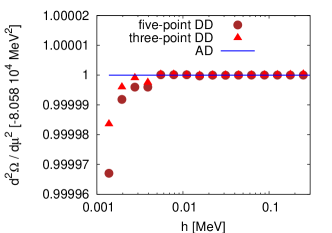
(a) Second-order derivative

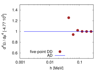
(b) Fourth-order derivative

Figure 1: Comparison of the second- (left) and fourth-order (right) derivatives of the grand potential $\bar{\Omega}$, evaluated at $(T,\mu)=(183,0)$ MeV, with respect to $\mu$ using three points and five points DD with the AD technique. All DD results are normalized to the AD results.

(a) Second-order derivative

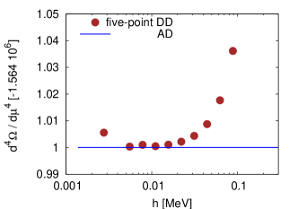
(b) Fourth-order derivative

Figure 2: Similar to Fig. 2 but $\bar{\Omega}$ evaluated at another point in the phase diagram, $(T,\mu)=(63,327)$ MeV.

As an example the corresponding approximations for the second derivative $f^{\prime\prime}(x)$ with three grid points $x_{i}$

$$f^{\prime\prime}(x)=\frac{1}{h^{2}}\left[f(x_{1})-2f(x_{2})+f(x_{3})\right]+\mathcal{O}(h^{2})$$ (28)

and with five grid points

$$f^{\prime\prime}(x)=\frac{1}{12h^{2}}\left[-f(x_{0})+16f(x_{1})\right.\\ \left.-30f(x_{2})+16f(x_{3})-f(x_{4})\right]+\mathcal{O}(h^{4})$$ (29)

are itemized. The grid points are given by

$$x_{0}=x-2h,\qquad x_{1}=x-h,\quad x_{2}=x$$

$$x_{3}=x+h,\quad x_{4}=x+2h\ .$$

For completeness the fourth-order derivative is quoted

$$f^{\prime\prime\prime\prime}(x)=\frac{1}{h^{4}}\left[f(x_{0})-4f(x_{1})+6f(x_{2})\right.\\ \left.-4f(x_{3})+f(x_{4})\right]+\mathcal{O}(h^{4})\ .$$ (30)

where at least five grid points are needed for its calculation.

The disadvantage of such type of improvements is that the function has to be evaluated at several different grid points $x_{i}$ which are located in the vicinity of $x$.

The other error source, the rounding error, depends on the used format of the floating point number representation in the computer. A single precision IEEE floating point number is stored in a 32-bit word, where 8 bits are used for the biased exponent and the fractional part of the normalized mantissa is a 23-bits binary number. One bit in the IEEE format is always reserved for the sign of the number. A double precision number occupies 64 bits, with the biased exponent stored in 11 bits and the fractional part is stored on the remaining 52 bits. Thus, besides the fact that one can represent only a finite subset of all real numbers, all floating point calculations are furthermore rounded resulting in incorrect values. The smallest positive number $\epsilon$, where the floating point approximation for $1+\epsilon$ is indeed larger than one is called the machine precision. When one rounds to the nearest representable number the machine precision is roughly $\epsilon\sim 2^{-m}$ where $m$ is the number of bits used to store the mantissa’s fraction. For a single precision representation one finds $\epsilon\sim 2^{-23}\sim 10^{-7}$ and for a double precision number calculation $\epsilon\sim 2^{-52}\sim 10^{-16}$. This means that single precision numbers have at most about 7 accurate digits while double precision numbers have about 16 accurate digits. But in general, due to the error propagation during the application of approximate algorithms the number of accurate digits for a numerical solution decreases. Therefore, the rounding error will be several orders of magnitude larger for a more complicated calculation such as the one for the thermodynamic potential. To minimize this source of error in the derivative calculation of the thermodynamic potential, a larger value of $h$ is reasonable.

In order to estimate these numerical errors and verify the quality of the ADOL-C evaluations the results of the derivative calculation obtained with AD are confronted with the DD method.

In Figs. 2 and 2 the results of a DD evaluation as a function of $h$ in comparison with the AD calculation for the second-order and fourth-order derivative of the thermodynamic potential are shown. Fig. 2 shows the $\mu$-derivatives of the potential evaluated at $(T,\mu)=(183,0)$ MeV which is close to the crossover phase transition in the $(T,\mu)$ phase diagram. One can clearly see the competition of the truncation and rounding errors. For the second-order derivative the optimal value is around $h\sim 0.05\,\text{MeV}$ while for the fourth-order derivative a slightly larger value $h\sim 0.1\,\text{MeV}$ leads to more stable results. In Fig. 2 the same derivatives are calculated at the point $(T,\mu)=(63,327)$ MeV which is near the critical end point in the phase diagram. While in the previous Fig. 2 the rounding error dominates, the truncation error is now more important. For the second-order derivative almost no rounding error is visible in the resolution shown. Since the truncation error for the five-point expression, Eq. (29), is of the order $\mathcal{O}\left(h^{4}\right)$ and of the order $\mathcal{O}\left(h^{2}\right)$ for the corresponding three-point equation, Eq. (28), the results of the five-point derivative is indistinguishable already for $h\sim 0.1\,\text{MeV}$ while for the three-point formula a smaller value of $h\sim 0.02\,\text{MeV}$ is required. For the fourth-order derivative the interval where the derivative does not vary with $h$ is very small. Only for $h\sim 0.01\,\text{MeV}$ the DD result is close to the AD result.

In summary, one realizes that the DD derivatives require a very careful fine-tuning of the $h$ value. The DD result coincides always with the DD results where the $h$ variation vanishes. One finds that the AD technique is more efficient than the DD method. The DD calculation always requires the evaluation of the function at several points, e.g., for the fourth derivative five function evaluations are necessary. In our case this involves the solution of the EoM at these five nodes. This is a time-consuming disadvantage of the DD method. With the AD the EoM need to be solved only once. Despite the fact that it is required to generate an internal function representation of the evaluation of the EoM solution and of the thermodynamic potential inside of ADOL-C, the AD implementation is much faster. Corresponding runtime measurements are illustrated in Fig. 3.

Figure 3: Runtime comparison for the DD and AD approaches.

The runtime of the DD approach can be described by the linear function $f(d)=m*d+a$ where as the AD runtime performs like $g(d)=c*\log_{2}(d)+b$. This result fits perfectly to the computational complexity of the AD approach described in Sec. 4.3.

6 Taylor coefficients

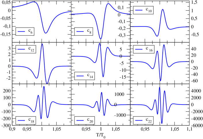
Figure 4: Taylor expansion coefficients $c_{6}(T)$ to $c_{22}(T)$ as a function of the temperature (see text for details).

As previously illustrated, both error sources for a derivative calculation with the DD method are in general difficult to keep under control, in particular, if higher-order derivatives are involved. However, with the AD method it is possible to obtain higher-order derivatives with very high precision. In the following an explicit example is given within the already introduced linear sigma model.

Higher derivatives are required if one is interested, e.g., in the extrapolation of Monte Carlo lattice simulations of strongly interacting matter (lattice gauge theory) to finite quark chemical potential. At finite quark chemical potential such types of Monte Carlo simulations cannot be directly performed [12]. One possible extrapolation to finite quark chemical potential is based on a Taylor expansion around zero chemical potential [13, 14].

For this purpose, we consider the same kind of expansion in the quark-meson system described by the L$\sigma$M. An example is given by the coefficients in the expansion of the pressure $p$ which is related to the thermodynamic potential via $p(T,\mu)=-\bar{\Omega}\left(T,\mu\right).$ At fixed temperature and small values of the quark chemical potential the pressure may be expanded in a Taylor series around $\mu=0$,

$$\frac{p(T,\mu)}{T^{4}}=\sum_{n=0}^{\infty}c_{n}(T)\left(\frac{\mu}{T}\right)^{n}\ ,$$ (31)

where the expansion coefficients are given in terms of derivatives of the pressure

$$c_{n}(T)=\left.\frac{1}{n!}\frac{\partial^{n}\left(p(T,\mu)/T^{4}\right)}{\partial\left(\mu/T\right)^{n}}\right|_{\mu=0}\ .$$ (32)

The series is even in $(\mu/T)$ which reflects the invariance of the partition function under the exchange of particles and antiparticles.

In Fig. 4 the expansion coefficients $c_{6}(T)$ to $c_{22}(T)$ are shown as function of the scaled temperature $T/T_{0}$. Here, $T_{0}$ is the pseudocritical temperature at which the crossover transition occurs for vanishing chemical potential. Since the first three expansion coefficients $c_{0},c_{2}$ and $c_{4}$ are already known and well-understood we do not show them again [12]. In lattice gauge theory one can currently calculate the first five coefficients, $c_{0},\ldots,c_{8}$ [15].

The higher coefficients $c_{n}$ with $n>4$ vanish for temperatures basically outside of a five percent window around $T_{0}$. Thus, all coefficients are only shown in the range $0.9<T/T_{0}<1.1$. All curves are smooth oscillating functions around zero even up to the $22^{\text{nd}}$ derivative order. The amplitude of the oscillation and the number of roots around $T_{0}$ increases with the order $n$. Thus, this oscillating behavior of the coefficients obviously requires a smaller $h$ in order to decrease the truncation error but then the rounding error increases. Already in this example the error sources are dramatic for such a high degree of derivatives. Therefore it is not reasonable and actually not possible to obtain the higher coefficients with standard techniques such as the DD method.

7 Summary

A novel numerical technique, which is based on algorithmic differentiation, for the calculation of arbitrarily high-order and high-precision derivatives has been presented. The new feature of the technique is the additional treatment of implicitly defined functions. In addition, the basic concepts of the algorithmic differentiation for explicit dependencies is discussed.

As a demonstration of the successful extension to implicitly defined functions the AD technique is applied to a quantum-field theoretical model for strongly-interacting matter. In this model the implicitly defined functions are represented by the underlying equations of motion where the implicitly defined order parameter is known only numerically.

Two important error sources namely, the rounding and truncation error, for a derivative calculation in general are discussed in detail. Furthermore, the results with the improved AD method are confronted to those obtained by standard divided difference (DD) methods. In the comparison the rounding and truncation errors can clearly be identified. While for a second-order derivative calculation the error sources are still controllable, they become intractable for higher orders.

In the model example higher-order derivative coefficients of a Taylor expansion for the pressure are calculated up to $22^{\text{nd}}$ order. Since these coefficients are calculated for the first time, no comparison with other results can be performed. The obtained curves are very stable and smooth functions which demonstrates the power of the novel AD technique. In a forthcoming publication [16] this method will be applied to the more realistic Polyakov-Quark-Meson model for three quark flavors [17, 18].

The presented AD technique augmented by implicitly defined dependencies can be applied to a wide class of problems, where high-order derivatives are involved. Standard alternative methods for the derivative calculation such as the DD method fail due to uncontrollably increasing errors. Especially, in the case of only numerically known implicit dependencies, an analytic solution is actually not possible. Here, the AD method is still applicable and displays its exceptional impact.

Acknowledgment

The work of MW was supported by the Alliance Program of the Helmholtz Association (HA216/ EMMI) and BMBF grants 06DA123 and 06DA9047I. We thank J. Albersmeyer, F. Karsch, A. Krassnigg, R. Roth and J. Wambach for useful discussions and comments.

References

- [1] Griewank, A. and Walther, A., Evaluating Derivatives: Principles and Techniques of Algorithmic Differentiation, 2nd ed., SIAM, Philadelphia, 2008.
- [2] Kedem, G., ACM Trans. Math. Softw. 6 (1980) 150.
- [3] www.Autodiff.org.
- [4] Gell-Mann, M. and Levy, M., Nuovo Cim. 16 (1960) 705.
- [5] Meyer-Ortmanns, H., Rev. Mod. Phys. 68 (1996) 473.
- [6] Schaefer, B.-J. and Wambach, J., Phys. Part. Nucl. 39 (2008) 1025.
- [7] Schaefer, B.-J. and Wagner, M., Phys. Rev. D79 (2009) 014018.
- [8] Brent, R. and Kung, H., J. Ass. Comp. Mach. 25 (1978) 581.
- [9] Griewank, A., Juedes, D., and Utke, J., ACM Trans. Math. Softw. 22 (1996) 131.
- [10] Griewank, A., Utke, J., and Walther, A., Math. of Comp. 69 (2000) 1117.
- [11] Press, W. H., Teukolsky, S. A., Vetterling, W. T., and Flannery, B. P., Numerical Recipes in C (2nd ed.): The art of scientific computing, Cambridge University Press, New York, NY, USA, 1992.
- [12] Philipsen, O., Eur. Phys. J. Spec. Top. 152 (2007) 29.
- [13] Allton, C. R. et al., Phys. Rev. D66 (2002) 074507.
- [14] Allton, C. R. et al., Phys. Rev. D71 (2005) 054508.
- [15] Miao, C. and Schmidt, C., PoS LAT2008 (2008) 172.
- [16] Karsch, F., Schaefer, B.-J., Wagner, M., and Wambach, J., in preparation, 2009.
- [17] Schaefer, B.-J. and Wagner, M., Prog. Part. Nucl. Phys. 62 (2009) 381.
- [18] Schaefer, B.-J., Wagner, M., and Wambach, J., arXiv:0910.5628 [hep-ph].