Superconductivity in a Two-Orbital Hubbard Model with Electron and Hole Fermi Pockets: Application in Iron Oxypnictide Superconductors

Abstract

We investigate the electronic states of a one-dimensional two-orbital Hubbard model with band splitting by the exact diagonalization method. The Luttinger liquid parameter $K_{\rho}$ is calculated to obtain superconducting (SC) phase diagram as a function of on-site interactions: the intra- and inter-orbital Coulomb $U$ and $U^{\prime}$, the Hund coupling $J$, and the pair transfer $J^{\prime}$. In this model, electron and hole Fermi pockets are produced when the Fermi level crosses both the upper and lower orbital bands. We find that the system shows two types of SC phases, the SC I for $U>U^{\prime}$ and the SC II for $U<U^{\prime}$, in the wide parameter region including both weak and strong correlation regimes. Pairing correlation functions indicate that the most dominant pairing for the SC I (SC II) is the intersite (on-site) intraorbital spin-singlet with (without) sign reversal of the order parameters between two Fermi pockets. The result of the SC I is consistent with the sign-reversing $s$-wave pairing that has recently been proposed for iron oxypnictide superconductors.

1 Introduction

The recent discovery of iron oxypnictide superconductors[1, 2, 3, 4, 5] with transition temperatures of up to $T_{c}\sim 55K$ has stimulated much interest in the relationship between the mechanism of the superconductivity and the orbital degrees of freedom. First-principles calculations have predicted the band structure with hole Fermi pockets around the $\Gamma$ point and electron Fermi pockets around the $M$ point[6, 7, 8]. By using the weak-coupling approaches based on multiorbital models, the spin-singlet $s$-wave pairing is predicted, where the order parameter of this pairing changes its sign between hole and electron Fermi pockets (sign-reversing $s$-wave pairing)[9, 10, 11, 12, 13]. This unconventional $s$-wave pairing is expected to emerge owing to the effect of antiferromagnetic spin fluctuations. Since the strong correlation between electrons is considered to play an important role in the superconductivity of iron oxypnictides as well as in that of high-$T_{c}$ cuprates, nonperturbative and reliable approaches are required.

As a nonperturbative approach, the exact diagonalization (ED) method has been extensively applied in the Hubbard, $d$-$p$, and $t$-$J$ models[14, 15]. Although these models are much simplified and mostly limited to one dimension, it has elucidated some important effects of a strong correlation on superconductivity. Using the ED method, we have studied the one-dimensional (1D) two-orbital Hubbard model in the presence of the band splitting $\Delta$. It is found that the superconducting (SC) phase appears in the vicinity of the partially polarized ferromagnetism when the exchange (Hund’s rule) coupling $J$ is larger than its critical value on the order of $\Delta$[16]. The result suggests that spin triplet pairing emerges owing to the effect of ferromagnetic spin fluctuation. In the case of $\Delta=0$, spin triplet superconductivity has also been discussed on the basis of bosonization[17, 18, 19] and numerical[20, 21, 22] approaches. Previous works, however, were restricted to the case of a single Fermi surface, and the effects of electron and hole Fermi pockets on superconductivity have not been discussed therein.

In this study, we investigate the 1D two-orbital Hubbard model with electron and hole Fermi pockets, where the Fermi level crosses both the upper and lower bands in the presence of a finite band splitting $\Delta$. Using the ED method, the Luttinger liquid parameter $K_{\rho}$ is calculated to obtain the SC phase diagram as a function of on-site Coulomb interactions in a wide parameter region including both weak- and strong-correlation regimes. It would clarify the effects of a strong correlation on superconductivity in iron oxypnictides. We also calculate various pairing correlation functions and discuss a possible pairing symmetry. Although our model is much simplified and limited to one dimension, we expect that the essence of the superconducting mechanism of iron oxypnictides can be discussed.

2 Model and Formulation

We consider the one-dimensional two-orbital Hubbard model given by the following Hamiltonian:

$$H = t\sum_{i,m,\sigma}(c_{i,m,\sigma}^{\dagger}c_{i+1,m,\sigma}+h.c.)$$ (1)

$$+ \frac{\Delta}{2}\sum_{i,\sigma}(n_{i,u,\sigma}-n_{i,l,\sigma})+U\sum_{i,m}n_{i,m,\uparrow}n_{i,m,\downarrow}$$

$$+ U^{\prime}\sum_{i,\sigma}n_{i,u,\sigma}n_{i,l,-\sigma}+(U^{\prime}-J)\sum_{i,\sigma}n_{i,u,\sigma}n_{i,l,\sigma}$$

$$- J\sum_{i}(c_{i,u,\uparrow}^{\dagger}c_{i,u,\downarrow}c_{i,l,\downarrow}^{\dagger}c_{i,l,\uparrow}+h.c.)$$

$$- J^{\prime}\sum_{i}(c_{i,u,\uparrow}^{\dagger}c_{i,u,\downarrow}^{\dagger}c_{i,l,\uparrow}c_{i,l,\downarrow}+h.c.),$$

where $c^{\dagger}_{i,m,\sigma}$ stands for the creation operator of an electron with a spin $\sigma\ (=\uparrow,\downarrow)$ and an orbital $m\ (=u,l)$ at site $i$ and $n_{i,m,\sigma}=c_{i,m,\sigma}^{\dagger}c_{i,m,\sigma}$. Here, $t$ represents the hopping integral between the same orbitals and we set $t=1$ in this study. The interaction parameters $U$, $U^{\prime}$, $J$, and $J^{\prime}$ stand for the intra- and inter-orbital direct Coulomb interactions, exchange (Hund’s rule) coupling, and pair-transfer, respectively. $\Delta$ denotes the energy difference between the two atomic orbitals. For simplicity, we impose the relation $J=J^{\prime}$.

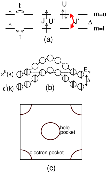
Figure 1: Schematic diagrams of (a) the model Hamiltonian, (b) the band structure in the noninteracting case, and (c) a corresponding two-dimensional Fermi surface related to our 1D model.

The model in eq. (1) is schematically shown in Fig. 1(a). In a noninteracting case ($U=U^{\prime}=J=0$), the Hamiltonian eq. (1) yields dispersion relations representing the upper and lower band energies: $\epsilon^{u}(k)=2t\cos(k)+\frac{\Delta}{2}$ and $\epsilon^{l}(k)=2t\cos(k)-\frac{\Delta}{2}$, where $k$ is the wave vector. This band structure is schematically shown in Fig. 1(b). When the Fermi level $E_{k_{\rm F}}$ crosses both the upper and lower bands, the system is metallic with electron and hole Fermi pockets corresponding to a characteristic band structure of the FeAs plane in iron oxypnictides, as shown in Fig. 1(c).

We numerically diagonalize the model Hamiltonian up to 6 sites (12 orbitals) and estimate the Luttinger liquid parameter $K_{\rho}$ from the ground-state energy of finite-size systems using the standard Lanczos algorithm.[14] To reduce the finite size effect, we impose the boundary condition (periodic or antiperiodic) on upper and lower orbitals independently and chose both boundary conditions to minimize $|K_{\rho}^{0}-1|$, where $K_{\rho}^{0}$ represents the $K_{\rho}$ of the finite-size system in a noninteracting case. The typical deviation of $K_{\rho}$ from unity becomes about $\sim 0.1$ for a six-site system. For simplicity, we will redefine $K_{\rho}$ as a renormalize value calculated using $K_{\rho}/K_{\rho}^{0}$, hereafter.

On the basis of the Tomonaga-Luttinger liquid theory [23, 24, 25, 26, 27], various types of correlation functions are determined by the single parameter $K_{\rho}$ in the model which is isotropic in spin space. For a single-band model with two Fermi points, $\pm k_{F}$, the SC correlation function decays as $\sim r^{-(1+\frac{1}{K_{\rho}})}$, while the CDW and SDW correlation functions decay as $\sim\cos({2k_{F}r})r^{-(1+K_{\rho})}$. Thus, the SC correlation is dominant for $K_{\rho}>1$, while the CDW or SDW correlation is dominant for $K_{\rho}<1$. On the other hand, for a two-band model with four Fermi points, i.e., $\pm k_{F_{1}}$ and $\pm k_{F_{2}}$, low-energy excitations are given by a single gapless charge mode with a gapped spin mode[26, 27, 28]. In this case, the SC and CDW correlations decay as $\sim r^{-\frac{1}{2K_{\rho}}}$ and $\sim\cos[{2(k_{F_{2}}-k_{F_{1}})r}]r^{-2K_{\rho}}$, respectively, while the SDW correlation decays exponentially. Hence, the SC correlation is dominant for $K_{\rho}>0.5$, while the CDW correlation is dominant for $K_{\rho}<0.5$. In either case, the SC correlation increases with the exponent $K_{\rho}$, and then $K_{\rho}$ is regarded as a good indicator of superconductivity.[29] As the noninteracting $K_{\rho}$ is always unity, we assume that the condition of $K_{\rho}>1$ for our model corresponds to the superconducting state realized in oxypnictide superconductors.

3 Phase Diagram

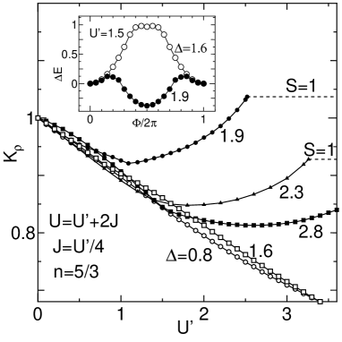
Figure 2: $K_{\rho}$ as a function of $U^{\prime}(=4J)$ for $n=5/3$ (10 electrons/6 sites) at $\Delta=0.8,1.6,1.9,2.3$, and 2.8. The singlet ground state changes into a partially polarized ferromagnetic ($S$=1) state at $U^{\prime}\simeq$ 2.5, 3.2, and 4.1 for $\Delta=$ 1.9, 2.3, and 2.8, respectively. The inset shows the energy difference $E_{0}(\phi)-E_{0}(0)$ as a function of the external flux $\phi$ for $n=2/3$ (6 electrons/9 sites) at $\Delta=1.2$.

Figure 2 shows $K_{\rho}$ as a function of $U^{\prime}$ for several values of $\Delta$ at an electron density $n=5/3$ (10 electrons/6 sites), where we set $J=U^{\prime}/4$ with $U=U^{\prime}+2J$. When $U^{\prime}$ increases, $K_{\rho}$ decreases for a small $U^{\prime}$, while it increases for a large $U^{\prime}$ in the case of $\Delta\geq 1.9$, and then becomes larger than unity for $U^{\prime}>2.3$ in the case of $\Delta=1.9$. When $J(=U^{\prime}/4)$ is larger than a certain critical value, the ground state changes into the partially polarized ferromagnetic state with a total spin $S=1$ from the singlet state with $S=0$. We find that superconductivity is most enhanced in the vicinity of the partially polarized ferromagnetic state. To confirm superconductivity, we calculate the energy difference of the ground state, $E_{0}(\phi)-E_{0}(0)$, as a function of the external flux $\phi$. As shown in the inset of Fig. 2, anomalous flux quantization is clearly observed for $\Delta=1.9$ while not for $\Delta=0.8$.

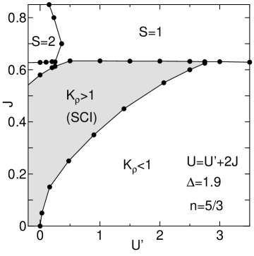
Figure 3: Phase diagram of the ground state with $K_{\rho}$ on the $U^{\prime}-J$ parameter plane with $U=U^{\prime}+2J$ for $n=5/3$ (10 electrons/6 sites) at $\Delta=1.9$.

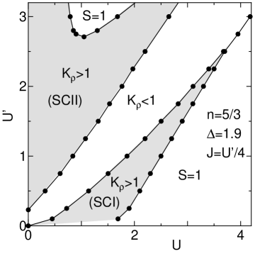
Figure 4: Phase diagram of the ground state with $K_{\rho}$ on the $U-U^{\prime}$ parameter plane with $J=U^{\prime}/4$ for $n=5/3$ (10 electrons/6 sites) at $\Delta=1.9$.

In Fig. 3, we show the phase diagram of the ground state on the $U^{\prime}-J$ parameter plane under the condition of $U=U^{\prime}+2J$ for $n=5/3$ (10 electrons/6 sites) at $\Delta=1.9$. It contains the singlet state with $S=0$ together with partially polarized ferromagnetic states with $S=1$ and $S=2$. The singlet state with $K_{\rho}>1$, where we call it the $SC$ phase, appears near the partially polarized ferromagnetic region at $J\stackrel{{\scriptstyle>}}{{{}_{\sim}}}U^{\prime}$. It extends from the attractive region ($U^{\prime}<0$) to the realistic parameter region with $J\sim U^{\prime}/4>0$, which is expected to correspond to that in the case of iron oxypnictides[8]. We have confirmed that similar phase diagrams are also obtained for $\Delta=2.3$ and 2.6.

Figure 4 shows the phase diagram of the ground state on the $U-U^{\prime}$ plane under the condition of $J=U^{\prime}/4$ for $n=5/3$ (10 electrons/6 sites) at $\Delta=1.9$. We observe two types of SC phases with $K_{\rho}>1$, the SC I for $U>U^{\prime}$ and the SC II for $U<U^{\prime}$, in the wide parameter region including both weak- and strong-correlation regimes. Note that the SC I corresponds to the SC phase shown in Fig. 3 and belongs to the realistic parameter region mentioned before.

4 Pairing Correlation

Figure 5: Schematic diagrams of various types of superconducting pairing symmetries, $S^{\rm l}_{\rm on}$, $S^{\rm u}_{\rm on}$, $S^{\rm l}_{\rm nn}$, $S^{\rm u}_{\rm nn}$, and $S^{\rm lu}_{\rm on}$ with spin singlet pairings and $T^{\rm l}_{\rm nn}$, $T^{\rm u}_{\rm nn}$, and $T^{\rm lu}_{\rm on}$ with spin triplet pairings.

To examine the nature of these SC phases, we calculate SC pairing correlation functions for the various types of pairing symmetries schematically shown in Fig. 5. Explicit forms of the SC pairing correlation functions $C(r)$ are given by

$$S^{\rm l}_{\rm on}(r) = \frac{1}{N}\sum_{i}\langle c^{\dagger}_{i,l,\uparrow}c^{\dagger}_{i,l,\downarrow}c_{i+r,l,\downarrow}c_{i+r,l,\uparrow}\rangle,$$

$$S^{\rm u}_{\rm on}(r) = \frac{1}{N}\sum_{i}\langle c^{\dagger}_{i,u,\uparrow}c^{\dagger}_{i,u,\downarrow}c_{i+r,u,\downarrow}c_{i+r,u,\uparrow}\rangle,$$

$$S^{\rm l}_{\rm nn}(r) = \frac{1}{2N}\sum_{i}\langle(c^{\dagger}_{i,l,\uparrow}c^{\dagger}_{i+1,l,\downarrow}-c^{\dagger}_{i,l,\downarrow}c^{\dagger}_{i+1,l,\uparrow})$$

$$\times (c_{i+r+1\downarrow}c_{i+r,l,\uparrow}-c_{i+r+1,l,\uparrow}c_{i+r,l,\downarrow})\rangle,$$

$$S^{\rm u}_{\rm nn}(r) = \frac{1}{2N}\sum_{i}\langle(c^{\dagger}_{i,u,\uparrow}c^{\dagger}_{i+1,u,\downarrow}-c^{\dagger}_{i,u,\downarrow}c^{\dagger}_{i+1,u,\uparrow})$$

$$\times (c_{i+r+1,u,\downarrow}c_{i+r,u,\uparrow}-c_{i+r+1,u,\uparrow}c_{i+r,u,\downarrow})\rangle,$$

$$S^{\rm lu}_{\rm on}(r) = \frac{1}{2N_{u}}\sum_{i}\langle(c^{\dagger}_{i,l,\uparrow}c^{\dagger}_{i,u,\downarrow}-c^{\dagger}_{i,l,\downarrow}c^{\dagger}_{i,u,\uparrow})$$

$$\times (c_{i+r,u,\downarrow}c_{i+r,l,\uparrow}-c_{i+r,u,\uparrow}c_{i+r,l,\downarrow})\rangle,$$

$$T^{\rm l}_{\rm nn}(r) = \frac{1}{2N_{u}}\sum_{i}\langle(c^{\dagger}_{i,l,\uparrow}c^{\dagger}_{i+1,l,\downarrow}+c^{\dagger}_{i,l,\downarrow}c^{\dagger}_{i+1,l,\uparrow})$$

$$\times (c_{i+r+1\downarrow}c_{i+r,l,\uparrow}+c_{i+r+1,l,\uparrow}c_{i+r,l,\downarrow})\rangle,$$

$$T^{\rm u}_{\rm nn}(r) = \frac{1}{2N_{u}}\sum_{i}\langle(c^{\dagger}_{i,u,\uparrow}c^{\dagger}_{i+1,u,\downarrow}+c^{\dagger}_{i,u,\downarrow}c^{\dagger}_{i+1,u,\uparrow})$$

$$\times (c_{i+r+1,u,\downarrow}c_{i+r,u,\uparrow}+c_{i+r+1,u,\uparrow}c_{i+r,u,\downarrow})\rangle,$$

$$T^{\rm lu}_{\rm on}(r) = \frac{1}{2N_{u}}\sum_{i}\langle(c^{\dagger}_{i,l,\uparrow}c^{\dagger}_{i,u,\downarrow}+c^{\dagger}_{i,l,\downarrow}c^{\dagger}_{i,u,\uparrow})$$

$$\times (c_{i+r,u,\downarrow}c_{i+r,l,\uparrow}+c_{i+r,u,\uparrow}c_{i+r,l,\downarrow})\rangle,$$

where $S^{\rm l}_{\rm on}(r)$, $S^{\rm u}_{\rm on}(r)$, $S^{\rm l}_{\rm nn}(r)$, $S^{\rm u}_{\rm nn}(r)$, and $S^{\rm lu}_{\rm on}(r)$ denote the singlet pairing correlation functions on the same site in the lower orbital, on the same site in the upper orbital, between nearest-neighbor sites in the lower orbital, between nearest-neighbor sites in the upper orbital, and between the lower and upper orbitals on the same site, respectively. Furthermore, $T^{\rm l}_{\rm nn}(r)$, $T^{\rm u}_{\rm nn}(r)$, and $T^{\rm lu}_{\rm on}(r)$ are the triplet pairing correlation functions between nearest-neighbor sites in the lower orbital, between nearest-neighbor sites in the upper orbital, and between the lower and upper orbitals on the same site, respectively.

In Fig. 6, we show the absolute values of various types of SC pairing correlation functions $|C(r)|$ for $n=5/3$ (10 electrons/6 sites) at $\Delta=1.9$, $U^{\prime}=4J=1.0$, and $U=-0.4$. Here, the electronic state of the system belongs to the SC II phase, although the phase diagram for $U<0$ is not explicitly shown in Fig. 4. Note that $|T^{\rm u}_{\rm nn}(r)|<10^{-4}$ and $S^{\rm lu}_{\rm on}(r=3)=T^{\rm lu}_{\rm on}(r=3)=0$, which are not shown in Fig. 6. We find that $S^{\rm u}_{\rm on}(r)$ and $S^{\rm u}_{\rm nn}(r)$ decay very slowly as functions of $r$, and $|S^{\rm u}_{\rm on}(r=3)|$ is the largest among the various $|C(r=3)|$ values. Therefore, a relevant pairing symmetry for the SC II phase seems to be the spin singlet pairing in the upper orbital band, mainly consist of ’on-site’ pairing. It is considered that such a pairing in attractive region with $U<0$ is due to the intra-orbital attraction $U$. On the other hand, in repulsive region with $U^{\prime}>U>0$, the pairing may be due to charge fluctuation, which is enhanced by a large inter-orbital repulsion $U^{\prime}$ similarly to that in the case of the $d$-$p$ model in the presence of the inter-orbital repulsion $U_{pd}$[30].

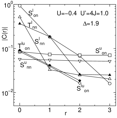
Figure 6: Absolute values of various types of SC pairing correlation functions $|C(r)|$ as functions of $r$ for $n$=5/3 (10 electrons/6 sites) at $\Delta=1.9$, $U^{\prime}(=4J)=1.0$, and $U=-0.4$, corresponding to the SC II phase.

Next, we discuss the superconductivity in the SC I phase including the realistic parameter region mentioned before. Figure. 7 shows the absolute values of various types of SC pairing correlation functions $|C(r)|$ for $n=5/3$ (10 electrons/6 sites) at $\Delta=1.9$, $U^{\prime}=4J=1.0$, and $U=2.4$, where the system belongs to the SC I phase, as shown in Fig. 4. Here, $|T^{\rm u}_{\rm nn}(r)|$, $|S^{\rm lu}_{\rm on}(r=3)|$, and $|T^{\rm lu}_{\rm on}(r=3)|$ are not shown, because these correlation functions are very small or zero. We find that $|S^{\rm u}_{\rm on}(r)|$ is considerably suppressed compared with $|S^{\rm u}_{\rm nn}(r)|$ in contrast to that in the case of the SC II phase. Furthermore, $|S^{\rm l}_{\rm nn}(r)|$ increases with increasing $r$ except at $r=2$. Therefore, the relevant pairing symmetry for the SC I phase seems to be an extended spin singlet pairing, and mainly consist of nearest-neighbor site pairing.

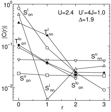
Figure 7: Absolute values of various types of SC pairing correlation functions $|C(r)|$ as functions of $r$ for $n$=5/3 (10 electrons/6 sites) at $\Delta=1.9$, $U^{\prime}(=4J)=1.0$, and $U=2.4$, corresponding to the SC I phase.

Recently, weak-coupling approaches such as RPA and perturbation expansions have shown that the sign-reversing $s$-wave ($s_{\pm}$-wave) pairing is realized in iron oxypnictide superconductors[9, 10, 11, 12, 13]. The order parameter of such a pairing is considered to change its sign between hole and the electron Fermi pockets. To compare our result with the result obtained by weak-coupling approaches, we examine the SC pairing correlation function between the $lower$ and $upper$ orbitals, such as

$$S^{\rm l-u}_{\rm nn}(r)=\frac{1}{2N}\sum_{i}<{\Delta^{l}_{\rm nn}(i)}^{\dagger}\Delta^{u}_{\rm nn}(i+r)>$$

with

$${\Delta^{m}_{\rm nn}(i)}^{\dagger}=c^{\dagger}_{i,m,\uparrow}c^{\dagger}_{i+1,m,\downarrow}-c^{\dagger}_{i,m,\downarrow}c^{\dagger}_{i+1,m,\uparrow}\ \ (m=l,u).$$

We also define $T^{\rm l-u}_{\rm nn}(r)$ as well as $S^{\rm l-u}_{\rm nn}(r)$ in the above equation.

When the $s_{\pm}$-wave pairing is dominant, the values of the interorbital SC pairing correlation function are expected to be negative, since the Fermi surface of the lower (upper) orbital band in our model corresponds to a hole (electron) Fermi pocket, as shown in Fig. 1(b). In Fig. 8, we show the interorbital pairing correlation functions $S^{\rm l-u}_{\rm nn}(r)$ and $T^{\rm l-u}_{\rm nn}(r)$(see also inset) for the same parameters in Fig. 4 corresponding to the SC I phase. We see that the values of $T^{\rm l-u}_{\rm nn}(r)$ are positive and very small, while those of $S^{\rm l-u}_{\rm nn}(r)$ are negative except at $r=3$ and not so small. This result suggests that the relevant pairing symmetry of the SC I phase is the spin-singlet $s_{\pm}$-wave pairing, which agrees with the result of the weak coupling approaches. Therefore, we expect that the $s_{\pm}$-wave pairing proposed on the basis of the result of weak-coupling approaches is realized in the wide parameter region including both weak- and strong-correlation regimes.

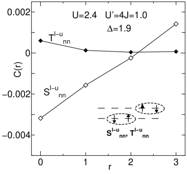
Figure 8: Pairing correlation functions $S^{\rm l-u}_{\rm nn}(r)$ and $T^{\rm l-u}_{\rm nn}(r)$. Here, we show the absolute value of the correlation functions at $U=2.4$, $\Delta=1.9$, and $U^{\prime}(=4J)=1.0$ for $n$=5/3 (10 electrons/6 sites). The inset shows a schematic diagram of the pairing symmetries, $S^{\rm l-u}_{\rm nn}(r)$ and $T^{\rm l-u}_{\rm nn}(r)$.

Finally, we discuss the mechanism of superconductivity in the SC I phase. The $s_{\pm}$-wave pairing is considered to be mediated by the antiferromagnetic fluctuation due to the nesting effect between electron and hole pockets [9, 10, 11, 12, 13]. At first glance, the SC I phase is located adjacent to the partial ferromagnetic phase (S=1), and then, the ferromagnetic fluctuation seems to be related to superconductivity. To examine the relationship between spin fluctuation and superconductivity, we also calculate the spin correlation function for finite-size systems, where a short-range spin correlation is considered to be crucial for the superconductivity. We obtain the ferromagnetic and antiferromagnetic components of the spin correlation as a function of $U^{\prime}(=4J)$ for a fixed $U=1.5$ (see also Fig. 4) and find that antiferromagnetic (ferromagnetic) correlation increases (decreases) with decreasing $U^{\prime}$ together with increasing $K_{\rho}$ (not shown). Therefore, we conclude that the antiferromagnetic spin fluctuation is responsible for the $s_{\pm}$-wave pairing in the SC I phase.

5 Summary and Discussion

We have investigated the superconductivity of the one-dimensional two-orbital Hubbard model in the case of electron and hole Fermi pockets corresponding to a characteristic band structure of iron oxypnictide superconductors. To obtain reliable results including those in the strong-correlation regime, we used the exact diagonalization method and calculated the critical exponent $K_{\rho}$ on the basis of the Luttinger liquid theory. It has been found that the system shows two types of SC phases, the SC I for $U>U^{\prime}$ and the SC II for $U<U^{\prime}$, in the wide parameter region including both weak- and strong-correlation regimes.

We have also calculated various types of SC pairing correlation functions in the realistic parameter region of the iron oxypnictides. The result indicates that the most dominant pairing for the SC I phase is the intersite intraorbital spin-singlet with sign reversal of the order parameters between two Fermi pockets. The result is consistent with the sign-reversing $s_{\pm}$-wave pairing that has recently been proposed on the basis of the result obtained by weak-coupling approaches for iron oxypnictide superconductors. This indicates that the $s_{\pm}$-wave pairing is realized not only in a weak-correlation regime but also in a strong-correlation regime. We have also calculated the spin correlation function and found that antiferromagnetic spin fluctuation is responsible for the $s_{\pm}$-wave pairing in the SC I phase.

As for the SC II phase, the most dominant pairing is found to be the on-site intraorbital spin-singlet pairing, which is consistent with the ordinary $s$-wave pairing of BCS superconductors. However, the superconducting mechanism of this phase is due to the charge fluctuation enhanced by the interorbital Coulomb interaction and is different from the conventional BCS superconductivity due to the electron-phonon interaction. Although the SC II phase seems to be realized only for the unrealistic parameter region in our model, it might be realized for a realistic parameter region in the $d$-$p$ model, which is closer to iron oxypnictides[13, 30]. We will address such a problem by applying the present method in the $d$-$p$ model in the future.

References

- [1] Y. Kamihara, T. Watanabe, M. Hirano, and H. Hosono: J. Am. Chem. Soc. 130 (2008) 3296.
- [2] Z.-A. Ren, W. Lu, J. Yang, W. Yi, X.-L. Shen, Z.-C. Li, G.-C. Che, X.-L. Dong, L.-L. Sun, F. Zhou, and X.-X. Zhao: Chin. Phys. Lett. 25 (2008) 2215.
- [3] X. H. Chen, T. Wu, G. Wu, R. H. Liu, H. Chen, and D. F. Fang: Nature 453 (2008) 761.
- [4] G. F. Chen, Z. Li, D. Wu, G. Li, W. Z. Hu, J. Dong, P. Zheng, J. L. Luo, and N. L. Wang: Phys. Rev. Lett. 100 (2008) 247002.
- [5] H. Kito, H. Eisaki, and A. Iyo: J. Phys. Soc. Jpn. 77 (2008) 063707.
- [6] D. J. Singh, and M. H. Du: Phys. Rev. Lett. 100 (2008) 237003.
- [7] S. Ishibashi, K. Terakura, and H. Hosono: J. Phys. Soc. Jpn. 77 (2008) 053709.
- [8] K. Nakamura, R. Arita, and M. Imada: J. Phys. Soc. Jpn. 77 (2008) 093711.
- [9] K. Kuroki, S. Onari, R. Arita, H. Usui, Y. Tanaka, H. Kontani, and H. Aoki: Phys. Rev. Lett. 101 (2008) 087004.
- [10] I. I. Mazin, D. J. Singh, M. D. Johannes, and M. H. Du: Phys. Rev. Lett. 101 (2008) 057003.
- [11] F. Wang, H. Zhai, Y. Ran, A. Vishwanath, and D.-H. Lee: Phys. Rev. Lett. 102 (2009) 047005.
- [12] T. Nomura: J. Phys. Soc. Jpn. 78 (2009) 034716; J. Phys. Soc. Jpn. 77 (2008) Suppl. C, 123.
- [13] Y. Yanagi, Y. Yamakawa, and Y. Ōno: J. Phys. Soc. Jpn. 77 (2008) 123701; J. Phys. Soc. Jpn. 77 (2008) Suppl. C, 149.
- [14] H. J. Schulz: Phys. Rev. Lett. 64 (1990) 2831; A. Sudbø, C.M. Varma, T. Giamarchi, E.B. Stechel and T. Scalettar: Phys. Rev. Lett. 70 (1993) 978; M. Ogata, M. U. Luchini, S. Sorella and F. F. Assaad: Phys. Rev. Lett. 66 (1991) 2388.
- [15] C. A. Hayward, D. Poilblanc, R. M. Noack, D. J. Scalapino, and W. Hanke: Phys. Rev. Lett. 75 (1995) 926; D. Poilblanc, D. J. Scalapino, and W. Hanke: Phys. Rev. B 52 (1995) 6796; K. Sano: J. Phys. Soc. Jpn. 65 (1996) 1146.
- [16] K. Sano and Y. Ōno: J. Phys. Soc. Jpn. 72 (2003) 1847; J. Phys. Condens. Matter 19 (2007) 14528.
- [17] D. G. Shelton and A. M. Tsvelik: Phys. Rev. B53 (1996) 14036.
- [18] S. Q. Shen; Phys. Rev. B57 (1998) 6474.
- [19] H. C. Lee, P. Azaria, and E. Boulat: Phys. Rev. B 69 (2004) 155109.
- [20] H. Sakamoto, T. Momoi, and K. Kubo: Phys. Rev. B 65 (2002) 224403.
- [21] T. Shirakawa, Y. Ohta, and S. Nishimoto: J. Mag. Mag. Mater. 310 (2) (2007) 663.
- [22] K. Sano and Y. Ōno: J. Mag. Mag. Mater. 310 (2) (2007) e319.
- [23] J. Solyom: Adv. Phys. 28 (1979) 201.
- [24] J. Voit: Rep. Prog. Phys. 58 (1995) 977.
- [25] V. J. Emery: in Highly Conducting One-Dimensional Solids, ed. J. T. Devreese, R. Evrand, and V. van Doren (Plenum, New York, 1979) p. 327.
- [26] L. Balentz and M. P. A. Fisher: Phys. Rev. B53 (1996) 12133.
- [27] M. Fabrizio: Phys. Rev. B 54 (1996) 10054.
- [28] V. J. Emery, S. A. Kivelson, and O. Zachar: Phys. Rev. B59 (1999) 15641.
- [29] The noninteracting band structure for the present model is almost equivalent to that for the ladder model, which has electron and hole Fermi pockets during moderate band splitting and filling. Results obtained using numerical methods such as the ED and DMRG indicate that the electronic state of the ladder model can be analyzed well using the weak-coupling theory except in a strong-coupling limit[15].
- [30] K. Sano and Y. Ōno: Physica C205 (1993) 170; Phys. Rev. B51 (1995) 1175; Physica C242 (1995) 113.