Relativistic particle acceleration in developing Alfvén turbulence

Abstract

A new particle acceleration process in a developing Alfvén turbulence in the course of successive parametric instabilities of a relativistic pair plasma is investigated by utilyzing one-dimensional electromagnetic full particle code. Coherent wave-particle interactions result in efficient particle acceleration leading to a power-law like energy distribution function. In the simulation high energy particles having large relativistic masses are preferentially accelerated as the turbulence spectrum evolves in time. Main acceleration mechanism is simultaneous relativistic resonance between a particle and two different waves. An analytical expression of maximum attainable energy in such wave-particle interactions is derived.

1 Introduction

Large amplitude Alfvén waves are ubiquitous in space and astrophysical environments. Such waves are believed to play key roles in the so-called DSA (diffusive shock acceleration) process in which charged particles are diffusively accelerated in the course of multiple scattering through turbulent Alfvén waves upstream and downstream of collisionless shocks. The DSA is widely accepted as one of the most efficient acceleration mechanisms of galactic cosmic rays of energy up to $\sim 10^{15.5}eV$ (Krymsky, 1977; Axford et al., 1977; Bell, 1978; Blandford & Ostriker, 1978; Drury, 1983; Lagage & Cesarsky, 1983; Blandford & Eichler, 1987; Jones & Ellison, 1991; Malkov & Drury, 2001; Duffy & Blundell, 2005). In the process it is implicitly assumed that the Alfvén turbulence is phase randomized and its spectrum is time stationary. On the other hand, turbulent Alfvén waves commonly observed in the solar-terrestrial environments are often intermittent, and coherent MHD structures are frequently superposed. Namely, the phase random approximation cannot be assumed (de Wit et al., 1999; Hada et al., 2003; Narita et al., 2006) and a spectrum of turbulence may evolve both in space and time (Bruno & Carbone, 2005). This is probably due to the fact that nonlinear wave-wave interactions tend to generate coherence among wave phases, and that spatial and temporal scales of relaxation processes in space plasmas are much larger than typical scales of our solar-terrestrial system. This may hold true with some high energy astrophysical environments. That is, spatial and temporal scales of a relaxation process are not negligibly small in comparison with scales of a whole acceleration site. Generally speaking, particle acceleration rate through coherent wave-particle interactions is much higher than that through incoherent, or fully turbulent, wave-particle interactions (Kuramitsu & Hada, 2000, 2008). Therefore, acceleration processes through coherent wave-particle interactions in a ’developing’ turbulence, where a turbulence has not been fully developed, should be paid more serious attention.

It is well-known that in various space plasma environments a nonequilibrium ion distribution function generates large amplitude Alfvén waves through some instabilities and that those waves nonlinearly evolve to produce coherent magnetic wave forms. One of the common interpretations of generation mechanisms of such wave forms accompanying density fluctuations which are frequently observed in the solar wind (Spangler et al., 1997; Spangler & Fuselier, 1988) is a parametric instability where nonlinear wave-wave interactions convert energy of a parent wave into several daughter waves with different frequencies and wavelengths (Galeev & Oraevskii, 1963; Sagdeev & Galeev, 1969). Although in the context of cosmic ray acceleration in turbulent media the above process was taken into account to estimate steady state distributions of wave intensities (Chin & Wentzel, 1972; Wentzel, 1974; Skilling, 1975a, b, c), its developing processes and associated coherent wave-particle interactions have never been considered. Recent numerical studies revealed that successive parametric instabilities result in turbulent wave forms which have not been fully developed (Matsukiyo & Hada, 2003; Nariyuki & Hada, 2005, 2006). However, only a few past studies paid much attention to particle acceleration processes in such a developing turbulence. Furthermore, only limited spatial and temporal evolutions of wave forms or spectra were discussed, since a computational resource was limited.

In this paper long time evolution of parametric instabilities of a large amplitude Alfvén wave in a rather large spatial domain is reproduced by utilizing one-dimensional relativistic full particle-in-cell (PIC) code. A plasma is assumed to be composed of electrons and positrons, since electron-positron pairs can be the dominant constituent of some high energy astrophysical plasmas like in the vicinity of a pulsar, active galactic nuclei (AGN), gamma ray burst (GRB), and so on. In the simulation we observe a particle acceleration process which is quite efficient and is due to interactions between coherent Alfvén waves and relativistic particles. The process is quite different from some other coherent acceleration processes being discussed recently, in which high frequency electrostatic waves play essential roles, like electron surfing acceleration induced by a cross field Buneman instability (Shimada & Hoshino, 2000; McClements et al., 2001; Hoshino & Shimada, 2002; Dieckmann et al., 2004, 2005; Amano & Hoshino, 2007) and wakefield acceleration (Tajima & Dawson, 1979; Katsouleas & Dawson, 1983; Lyubarsky, 2006; Hoshino, 2008).

Simulation settings and results are represented in section 2. The acceleration process is discussed in detail by using an analytical model and test particle simulation in section 3. Summary and discussions are given in section 4.

2 1D PIC Simulation

Long time evolution of parametric instabilities of a large amplitude monochromatic Alfvén wave in a relativistic pair plasma is reproduced by performing a one-dimensional PIC simulation. A parent wave is given only at the beginning of the run as a monochromatic and right-handed circularly polarized Alfvén wave with amplitude $B_{p}/B_{0}=1$ and wavenumber $k_{0}c/\Omega_{0}=6.21$ (number of wave mode is 512) which gives a frequency $\omega_{0}/\Omega_{0}=0.627$, where ${\bf B_{0}}$ is the ambient magnetic field which is along the $x-$axis, $c$ denotes speed of light, and $\Omega_{0}=eB_{0}/m_{0}c$ is nonrelativistic gyrofrequency, respectively. Corresponding velocity perturbations of the pair plasma are given by the relativistic Walen relation (Hada et al., 2004). Boundary conditions are periodic for particles and all field components. System size is $L=518.1c/\Omega_{0}$. Squared ratio of nonrelativistic gyro and plasma frequencies is $\Omega^{2}_{0}/\omega^{2}_{p}=0.1$, and normalized scalar temperature for both electrons and positrons is $T/m_{0}c^{2}=1.6\times 10^{-3}$.

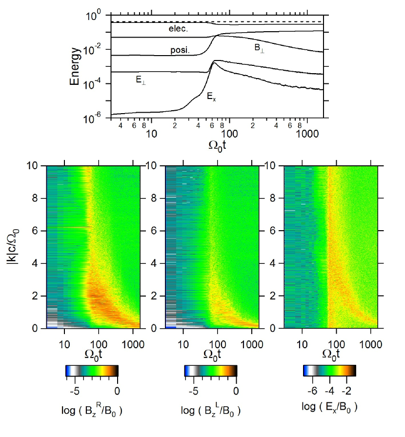
Figure 1: Time evolution of wave power spectra. The right and left hand helicity modes of $B_{z}$ component are Fourier decomposed in left and middle panels, respectively. The right panel shows $E_{x}$ component. See the electronic edition of the Journal for a color version of this figure.

Fig.1 shows time evolutions of energy densities (upper panel) and Fourier spectra of wave amplitudes for $B_{z}$ and $E_{x}$ field components (lower panels). In the upper panel the solid lines denote electron and positron kinetic energies (labeled by ‘elec.’ and ‘posi.’), transverse magnetic field energy (‘$B_{\perp}$’), and transverse and longitudinal electric field energies (‘$E_{\perp}$’ and ‘$E_{x}$’), respectively. The dashed line indicates the total energy, which is well conserved during the run. Although rather long system evolution (up to $\Omega_{0}t=1616$) is calculated, the system is still far from the so-called equilibrium state. In the lower panels wave amplitude spectra for positive and negative helicity (corresponding to positive and negative wavenumbers respectively) modes of the $B_{z}$ component are shown in the left ($B^{R}_{z}$) and middle ($B^{L}_{z}$) panels by using a technique of Fourier decomposition (Terasawa et al., 1986). Note that in the middle panel the actual sign of the wavenumber is negative. Since most of the daughter waves are right-hand polarized, the left (middle) panel shows wave intensity mainly of positively (negatively) propagating waves. At the beginning only the parent wave has significant intensity at $kc/\Omega_{0}=6.21$ in the left panel, although it is not particularly outstanding in the figure because of the narrow spectrum. In the early stage, $50<\Omega_{0}t<100$, the parent wave energy is transfered to a variety of daughter waves through large number of channels of wave-wave interactions. In this stage two parametric instabilities are dominant. A modulational instability generates daughter magnetic fluctuations with the same signs of wavenumber as that of the parent wave. They are observed in the $B^{R}_{z}$ spectrum. Couplings among the daughter and the parent waves result in compressional electrostatic fluctuations with wavenumber smaller than that of the parent wave as seen in the right panel. In a decay instability, on the other hand, daughter magnetic fluctuations have negative wavenumbers which appear in the $B^{L}_{Z}$ spectrum, while daughter electrostatic fluctuations have wavenumbers larger than that of the parent wave in the right panel. Most of the parent wave energy is wasted in this stage. However, the intensities of the daughter waves are still large so that successive parametric instabilities occur thereafter. These successive processes are sustained mainly by decay instabilities which can be confirmed because peak wavenumbers of the $E_{x}$ spectrum is always larger than those of the $B^{R}_{z}$ and $B^{L}_{z}$ spectra. The previous simulation study by Matsukiyo & Hada (2003) confirmed occurence of up to the second decay instability for the case of $B_{p}/B_{0}=0.1$.

Fig.2a demonstrates electron energy distribution functions at various times. Fourier amplitude spectra of $B_{z}$ component at the corresponding times are plotted in Fig.2b. Rapid heating occurs after the first instabilities developed ($\Omega_{0}t=95$: black dashed line). Up to this stage, most of the electrons show semi-stochastic motions in a noizy system with a primary wave. Here we refer the primary wave and the noize to the parent wave and superposition of the daughter waves, respectively. This results in rapid scattering in pitch angle as shown in Fig.2c, where an average pitch angle of electrons with respect to ${\bf B_{0}}$ and its standard deviation are plotted as a function of time. The standard deviation just after its rapid growth at $\Omega_{0}t\sim 70$ is $\sim 0.5$, which roughly coincides with an analytical estimate of the maximum pitch angle width of an electron resonating with the monochromatic parent wave (see Appendix). After the parent wave disappears, most of the electrons are detrapped by the parent wave and start to wander in the phase space. As time passes, a high energy tail appears in the electron distribution function (Fig.2a), which gradually approaches a power-law spectrum with index $\alpha\sim-2.5$ ($\Omega_{0}t=316$: gray solid line, $1616$: black solid line). At the same time the wave amplitude spectrum develops the power-law type spectrum also, with the index $\alpha\sim-2.0$, while the wave spectral peak shifts toward lower wavenumbers.

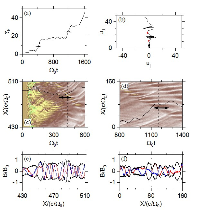
Figure 3: Behaviours of an accelerated electron. (a) Time history of the electron energy. (b) Trajectories of the electron in $u_{\perp}-u_{\parallel}$ space and (c)(d) in $X-t$ space. The arrows in (c) and (d) indicate time domains where strong acceleration occur as shown by the arrows in (a). Background color scale in (c) and (d) denotes amplitude of magnetic fluctuations. (e)(f) Spatial profiles of magnetic fluctuations in two acceleration phases represented by dashed lines in (c) and (d). The red, blue, and black solid lines show $B_{y}$, $B_{z}$ components and envelope, respectively. The dotted lines show positions of the particle at correspponding times. See the electronic edition of the Journal for a color version of this figure.

A behaviour of the most efficiently accelerated electron is shown in Fig.3. Fig.3a indicates energy time history of the electron. Spatial trajectory of the electron during $0<\Omega_{0}t<600$ ($800<\Omega_{0}t<1400$) is plotted in Fig.3c(d). A background color scale denotes strength of magnetic fluctuations $B_{\perp}\equiv\sqrt{B^{2}_{y}+B^{2}_{z}}$. Horizontal arrows in Fig.3c(d) and Fig.3a correspond to each other denoting time intervals where strong accelerations occur. Fig.3e(f) shows a snapshot of the wave profile at the time denoted as the dashed line in Fig.3c(d). The red, blue, and black lines represent $B_{y}$, $B_{z}$, and an envelope, respectively. The dotted line indicates the position of the electron. It is seen that strong acceleration occurs when the electron is trapped in a trough of the magnetic envelope. Such sharp envelope troughs are temporarily observed in various regions of the system throughout the run. Hence, the electron experiences similar acceleration processes several times. In this example one may recognize four such acceleration periods. Only the second and the third periods are marked (the first (fourth) one is $160<\Omega_{0}t<190$ ($\Omega_{0}t>1450$)). The acceleration occurs always perpendicular to ${\bf B_{0}}$ as seen in Fig.3b which shows a trajectory of the electron in the $u_{\perp}-u_{\parallel}$ space, where $u_{\perp}$ and $u_{\parallel}$ denote the four-velocities perpendicular and parallel to ${\bf B_{0}}$. The red markers indicate positions of the electron in the phase space at the same time as Fig.3e (lower marker) and Fig.3f (upper marker). We checked a hundred most efficiently accelerated electrons’ trajectories and confirmed that all of them show essentially the same features as mentioned above, i.e., trapping within the envelope troughs and successive perpendicular acceleration. In the next section the acceleration process is modeled and analyzed in detail.

3 Acceleration of High Energy Electrons

3.1 Coherent waves observed in the simulation: modeling

In the PIC simulation shown above sharp magnetic envelope troughs are locally formed throughout the period of strong electron accelerations. In a successive decay process a number of daughter Alfvén waves propagating both parallel and antiparallel to ${\bf B_{0}}$ are excited. Depending on their phases, amplitudes of some wave modes are sometimes locally canceled out each other, or they are simply less dominant in amplitude. Then, there appear some regions where two oppositely propagating waves dominate. Here, the envelope structures observed in the PIC simulation are modeled by a superposition of such two oppositely propagating waves as follows.

$$\left(\begin{array}[]{c}B^{y}_{w}\\ B^{z}_{w}\\ \end{array}\right)=B_{w}\cos kx\left(\begin{array}[]{c}{\cos\omega t}\\ {\sin\omega t}\\ \end{array}\right)\hskip 19.91692pt$$ (1)

$$\left(\begin{array}[]{c}E^{y}_{w}\\ E^{z}_{w}\\ \end{array}\right)=-{\omega\over kc}B_{w}\sin kx\left(\begin{array}[]{c}{\cos\omega t}\\ {\sin\omega t}\\ \end{array}\right)$$ (2)

Eq.(1) is equivallent to

$${\bf B_{w}}={B_{w}\over 2}\left(\begin{array}[]{c}{\cos(kx-\omega t)}\\ -{\sin(kx-\omega t)}\\ \end{array}\right)+{B_{w}\over 2}\left(\begin{array}[]{c}{\cos(-kx-\omega t)}\\ -{\sin(-kx-\omega t)}\\ \end{array}\right).$$

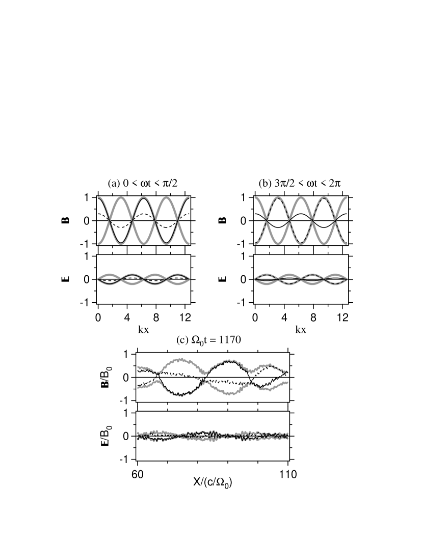
Figure 4: (a), (b) Modeled wave forms at different time domains ($B_{w}=1,\omega/kc=0.2$), and (c) an example of a waveform seen in the PIC simulation at $\Omega_{0}t=1170$.

Hereafter, we assume $\omega$ and $k$ are both positive without losing generality. Typical waveforms at two different time domains are shown in Fig.4a and b. The black solid and dashed lines denote $y$ and $z$ components of rotating carrier waves, and the gray lines represent envelopes which is independent of time. In the neighborhood of a trough, it is confirmed that eqs.(1) and (2) give a reasonable model of a waveform observed in the PIC simulation shown in Fig.4c. In the following motion of a test particle in this system is analyzed.

3.2 Motion of a particle in given EM fields

In this section we consider motion of an electron in the electromagnetic waves given by eqs.(1) and (2). The equation of motion is

$${d{\bf u}\over dt}=-{e\over m_{0}c}\left({\bf E}+{{\bf u}\over\gamma}\times{\bf B}\right),$$ (3)

$${dx\over dt}={u_{x}\over\gamma}c,$$ (4)

where ${\bf u}\equiv\gamma{\bf v}/c$, $\gamma=\sqrt{1+u^{2}}$, $e$ and $m_{0}$ indicate charge and rest mass of the electron, ${\bf B}=B_{0}{\bf x}+{\bf B_{w}}$, and ${\bf E}={\bf E_{w}}$, respectively. When we write ${\bf u}=(u_{\parallel}(t),u_{\perp}(t)\cos\phi(t),u_{\perp}(t)\sin\phi(t))$ and introduce normalized variables as $\xi=x\Omega_{0}/c$, $\tau=\Omega_{0}t$, $\kappa=kc/\Omega_{0}$, $\nu=\omega/\Omega_{0}$, $b_{w}=B_{w}/B_{0}$, and $v_{ph}=\nu/\kappa$, eqs.(3) and (4) are written as follows.

$$\dot{u}_{\parallel}=b_{w}{u_{\perp}\over\gamma}\cos\kappa\xi\sin\psi$$ (5)

$$\dot{u}_{\perp}=b_{w}\left(v_{ph}\sin\kappa\xi\cos\psi-{u_{\parallel}\over\ \gamma}\cos\kappa\xi\sin\psi\right),$$ (6)

$$\dot{\psi}=-{b_{w}\over u_{\perp}}\left(v_{ph}\sin\kappa\xi\sin\psi+{u_{\parallel}\over\ \gamma}\cos\kappa\xi\cos\psi\right)-\left(\nu-{1\over\gamma}\right).$$ (7)

$$\dot{\xi}={u_{\parallel}\over\gamma}.$$ (8)

Here, $\psi=\phi-\nu\tau$, and the dot denotes time derivative in terms of $\tau$, respectively. Note that a variation of normalized particle energy, or the Lorentz factor, is given as

$$\dot{\gamma}=b_{w}v_{ph}{u_{\perp}\over\gamma}\sin\kappa\xi\cos\psi.$$ (9)

In the following behaviours of the electron is discussed by using eqs.(5)-(9).

3.3 Fixed point analysis

The above set of equations clearly has several fixed points as listed in Table 1. Here, $u_{0}$ denotes a value of $u_{\perp}$ at a corresponding fixed point and $\gamma_{0}=\sqrt{1+u^{2}_{0}}$. Apparently, the fixed points I - III (IV - VI) correspond to troughs (crests) of the magnetic envelope. As far as the acceleration is concerned, it is easily inferred that the fixed points IV - VI are not important since the electric field strength is very weak around there. Actually, efficient acceleration observed in the PIC simulation always occurs around the troughs of the magnetic envelope. Therefore, only the fixed points I - III are focused here. Stability of these fixed points is discussed in the following.

3.3.1 Stability of the fixed points I - III

Expanding eqs.(5)-(9) around the fixed point I and retaining only the first order terms, we obtain

$$\delta\dot{u}_{\parallel}=-b_{w}{u_{0}\over\gamma_{0}}\kappa\delta\xi,$$ (10)

$$\delta\dot{u}_{\perp}=-b_{w}v_{ph}\delta\psi,$$ (11)

$$\delta\dot{\psi}={b_{w}\over u^{2}_{0}}v_{ph}\delta u_{\perp}-{1\over\gamma^{2}_{0}}\delta\gamma,$$ (12)

$$\delta\dot{\xi}={\delta u_{\parallel}\over\gamma_{0}}$$ (13)

$$\delta\dot{\gamma}=-b_{w}{u_{0}\over\gamma_{0}}v_{ph}\delta\psi={u_{0}\over\gamma_{0}}\delta\dot{u}_{\perp},$$ (14)

where $\delta$ denotes small first order quantities.

From eqs.(10) and (13), we have

$$\delta\ddot{u}_{\parallel}=-b_{w}{u_{0}\over\gamma^{2}_{0}}\kappa\delta u_{\parallel}.$$ (15)

The above expression represents a trapping oscillation with trapping frequency $\omega_{trap}=(b_{w}u_{0}\kappa/\gamma^{2}_{0})^{1/2}$, which is rewritten with the original parameters as $\omega_{trap}=(B_{w}kcu_{0}/B_{0}\Omega_{0}\gamma^{2}_{0})^{1/2}$.

From eqs.(11), (12), and (14), on the other hand, we obtain

$$\delta\ddot{u}_{\perp}={b_{w}u_{0}v_{ph}\over\gamma^{3}_{0}}\left(1-b_{w}v_{ph}{\gamma^{3}_{0}\over u^{3}_{0}}\right)\delta u_{\perp}.$$ (16)

Here, the first term in the parenthesis (or the second term in the right hand side of eq.(12)) arises from the variation of the Lorentz factor, i.e., due to the relativistic effect. In the non-relativistic limit, therefore, eq.(16) represents a trapping motion in the perpendicular momentum space with frequency $\omega_{trap}=b_{w}v_{ph}/u_{0}=(B_{w}/B_{0})(\omega/kc)(1/u_{0})$. However, in the relativistic case with $b_{w}v_{ph}\gamma^{3}_{0}/u^{3}_{0}<1$, $\delta u_{\perp}$ (and $\delta\psi$) diverges in time. When $u_{0}$ is small enough so that $\gamma_{0}\approx 1$, the above inequality is hardly satisfied. In such a case, the fixed point is stable. But if $u_{0}$ becomes large and the inequality is satisfied, such an electron gains transverse energy while it keeps being trapped in the $x-$direction. We consider this solution later more in detail.

For the fixed point II, equations corresponding to eqs.(15) and (16) are obtained by formally changing the sign of $b_{w}$. Therefore, the system is unstable for parallel fluctuations while it is stable for perpendicular fluctuations. This fixed point is actually conjugate to the relativistic fixed point discussed above. Another fixed point (III), conjugate to the nonrelativistic one, which should be a saddle point in $u_{\perp}-\psi$ phase space, appears at $(u_{\perp},\psi)=(0,n\pi)$ as singular points of $du_{\perp}/d\psi$, where $n=0,\pm 1,\pm 2,\cdots$.

3.3.2 Features in $u_{\perp}-\psi$ phase space

In order to study perpendicular dynamics let us first consider a reduced system in which parallel quantities are fixed at the fixed point, i.e., $u_{\parallel}=0$ and $\kappa\xi=\pi/2$. Then we only have to consider the following two equations.

$$\dot{p}=2\sqrt{p}b_{w}v_{ph}\cos\psi$$ (17)

$$\dot{\psi}=-{b_{w}\over\sqrt{p}}v_{ph}\sin\psi-\left(\nu-{1\over\sqrt{1+p}}\right)$$ (18)

Here, $p=u^{2}_{\perp}$ has been introduced. This system has a Hamiltonian defined as

$$H(p,\psi)=2\sqrt{p}b_{w}v_{ph}\sin\psi+\nu p-2\sqrt{1+p},$$ (19)

where $\dot{p}=\partial H/\partial\psi$ and $\dot{\psi}=-\partial H/\partial p$ are satisfied. Contours of the Hamiltonian for $b_{w}=1.0$, $v_{ph}=0.17$, and $\nu=0.11$ are represented as gray lines of the upper (linear scale) and lower panels (logarithmic scale) in Fig.5a. The above parameters are chosen so that the waves interacting with the accelerated electron in the second acceleration stage observed in the PIC simulation (Fig.3e) is appropriately reproduced. It is easily confirmed that a center at $\psi=\pi/2$, which is clearly recognized in the lower panel, corresponds to the nonrelativistic stable fixed point of the fixed point I and another center at $\psi=3\pi/2$, which can be seen both in the upper and lower panels, to the relativistic fixed point II discussed above.

The nonrelativistic center should satisfy the following condition from Table 1.

$$-{b_{w}v_{ph}\over u_{0}}=\nu-{1\over\gamma_{0}}$$ (20)

Although $\nu-1/\gamma_{0}=0$ in the small amplitude limit, it is never satisfied in the nonrelativistic case since $\nu<1$. Therefore, the nonrelativistic center appears only when wave amplitude becomes finite. The closed trajectories around this center essentially coincides with the nonresonant trapping discussed by Kuramitsu & Krasnoselskikh (2005).

At the relativistic center, the resonance condition $\nu-1/\gamma_{0}=0$ should be satisfied in the ultrarelativistic limit, since $b_{w}v_{ph}/u_{0}$ is negligible. In such a case relativistic decrease of the gyro frequency allows another resonance with low frequency waves. This resonance can also be present in small amplitude limit. Relativistic linear resonance conditions between an electron and two oppositely propagating waves ($\gamma\nu\mp\kappa u_{\parallel}-1=0$) are shown in Fig.5c. The two resonance lines intersect at $u_{\parallel}=0$ where $\nu-1/\gamma=0$ and $\gamma=\sqrt{1+u^{2}_{\perp}}$ are satisfied, while there never appears such an intersection in nonrelativistic limit. This indicates that an electron can resonate simultaneously with two waves in the relativistic case. By using eq.(19), the maximum width of the separatrix in $u_{\perp}$ is estimated as

$$\Delta u_{\perp}=4\sqrt{{b_{w}\over\kappa\nu}}.$$ (21)

Furthermore, the maximum $u_{\perp}$ on the separatrix is given by

$$u_{\perp,max}=\left(\sqrt{{b_{w}\over\kappa}}+\sqrt{{1\over\nu}}\right)^{2}=\left(\sqrt{{B_{w}\over B_{0}}{\Omega_{0}\over kc}}+\sqrt{\Omega_{0}\over\omega}\right)^{2}.$$ (22)

For instance, $u_{\perp,max}\approx 18.4$ for the parameters used in Fig.5. This gives a good agreement with the electron energy achieved in the end of the second acceleration stage observed in the PIC simulation.

So far we have only looked at a subset of the system in which $\delta u_{\parallel}=0$. If we allow $\delta u_{\parallel}$ to slightly deviated from zero, it should satisfy

$$\delta\ddot{u}_{\parallel}=-b_{w}{u_{0}\over\gamma^{2}_{0}}\kappa\sin\psi\delta u_{\parallel}$$ (23)

around the fixed point in the original system eqs.(5)-(8). Hence, the system is stable for $0<\psi<\pi$ and is unstable for $\pi<\psi<2\pi$ in terms of parallel fluctuations. The black solid line in Fig.5a and 5b shows a numerical solution of eqs.(5)-(8). A trajectory of the electron initially positioned near the separatrix at $\psi=0$ (indecated by a small arrow in Fig.5a) is represented. The electron moves alomost along the separatrix when it is in $0<\psi(<\pi)$. But when the electron enters in $\pi<\psi<2\pi$, its trajectory starts deviating from the separatrix. And finally it is clearly detrapped when it approaches $\psi=3\pi/2$. The trajectory in the momentum space shown in Fig. 5b is very similar to what is observed in the PIC simulation which is again plotted as a gray line.

3.4 Statistics of high energy particles

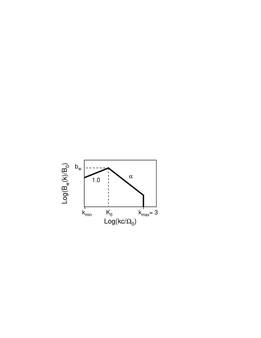
Figure 6: Wave power spectrum used in the test particle simulation.

Let us briefly discuss the power-law like distribution of electorns in the current acceleration process. It is shown in Fig.2a that a high energy tail with power-law index $\sim-2.5$ evolves in the late stage of the simulation. This power-law nature may be related with power-law spectrum of wave amplitude of magnetic fluctuations. In the stage of successive decay instabilities ($\Omega_{0}t>100$) a spectral cascade of the magnetic fluctuations occurs with keeping a power-law index of the wave amplitudes almost constant with $\sim-2.0$ (Fig.2b). The enhancement of the wave amplitude at higher wavenumber regime, $kc/\Omega_{0}>3$, is the remnant of initial parent wave and side band waves generated by the modulational instabilities in the early stage of the run. In order to confirm correlations between the wave and electron energy spectra, the following test particle simulation with periodic boundary conditions is performed. Waves are given by superposition of a number of right hand polarized Alfvén waves with power-law spectrum shown in Fig.6 (power-law index $\alpha$ is an external parameter), which models the lower wavenumber part of Fig.2b. Both positive and negative wavenumber modes are evenly distributed. The wave form is given by

$$\left(\begin{array}[]{c}B_{y}\\ B_{z}\\ \end{array}\right)=\sum^{3}_{kc/\Omega_{0}=-3}b_{w}B_{0}\left|{k\over K_{0}}\right|^{\alpha}\left(\begin{array}[]{c}\sin(k(x-v_{ph}t)+\Phi_{k})\\ \cos(k(x-v_{ph}t)+\Phi_{k})\\ \end{array}\right),$$ (24)

where $v_{ph}/c=0.17$ and $\{\Phi_{k}\}$ are initial wave phases which are randomly distributed at $t=0$, and corresponding transverse electric fields are given by ${\bf k}\times{\bf E}=(|k|v_{ph}/c){\bf B}$. The power-law index $\alpha$ is fixed to 1.0 for $k_{min}\leq k\leq K_{0}$, where $k_{min}\equiv 2\pi/L$ and $K_{0}$ is the coherence wavenumber. The system size $L=80\pi c/\Omega_{0}$ is common for all the following runs, and $b_{w}=0.75$ and $K_{0}c/\Omega_{0}=0.1$ if not specified.

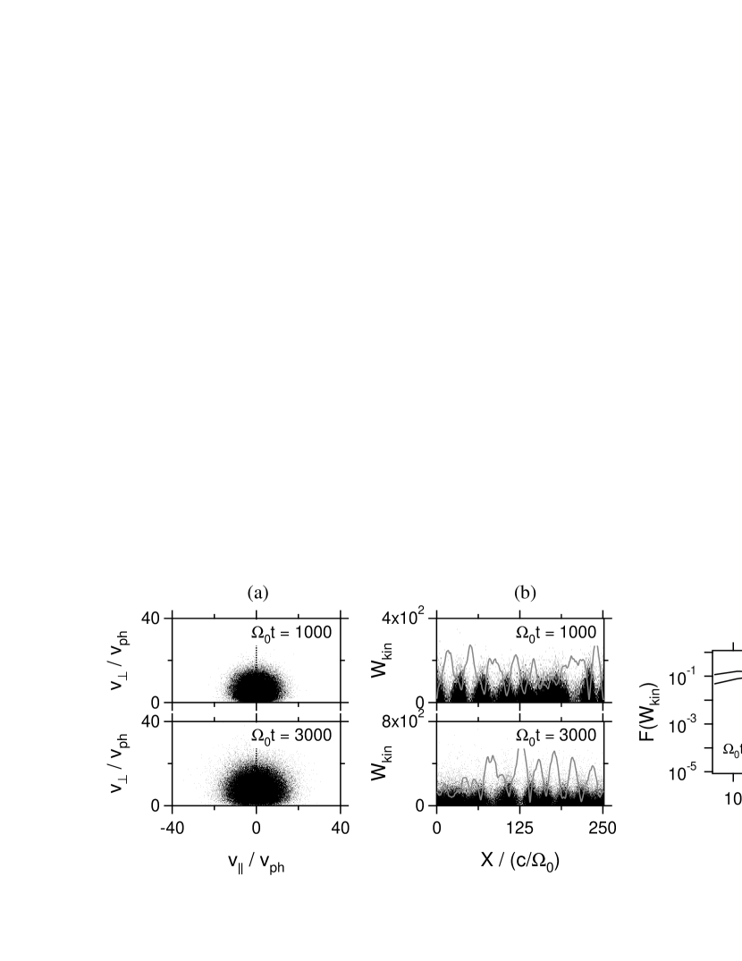
Figure 7: Results of nonrelativistic test particle simulation. Electron distributions in (a) $v_{\perp}-v_{\parallel}$ and (b) $X-W_{kin}$ phase spaces, and (c) energy distribution functions at $\Omega_{0}t=1000$ and $3000$, respectively. The solid gray lines in (b) denote profiles of magnetic field envelopes at the corresponding times.

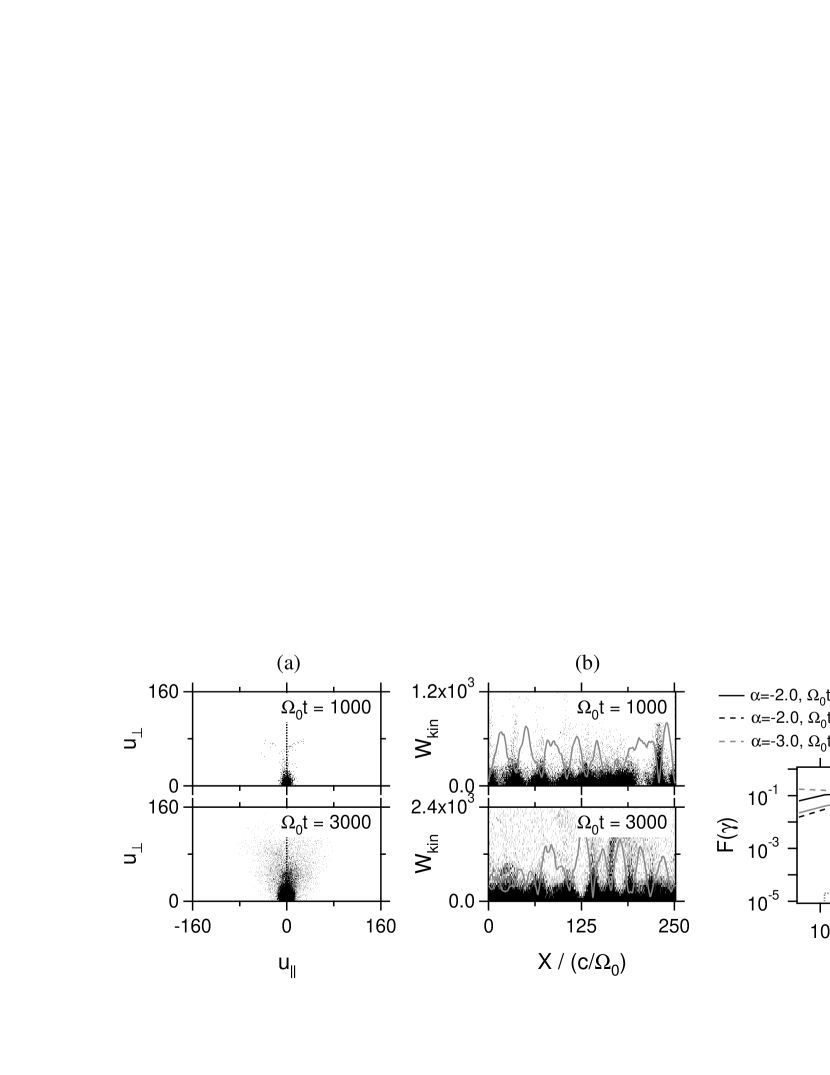
Figure 8: Results of relativistic test particle simulation in the same format as Fig.7. A number of energy distribution functions are plotted in (c). See datails in the text.

In such a system where a number of waves propagate in two opposite directions, particles are expected to be stochastically accelerated via second order Fermi like process. First, this is confirmed by solving nonrelativistic equations of motion of $10^{5}$ electrons. An initial distribution function is given as a spatially homogeneous gyrotropic ring distribution with $v_{\perp}/v_{ph}=0.1$. Fig.7 shows distributions in (a) $v_{\perp}-v_{\parallel}$ and (b) $X-W_{kin}$ phase spaces, and (c) energy distribution functions at two different times, $\Omega_{0}t=1000$ and $3000$, respectively, where ${\bf v}=(v_{\parallel},v_{\perp})$ denotes particle velocity and $W_{kin}=v^{2}/2v^{2}_{ph}$ is normalized kinetic energy. The solid gray lines in Fig.7b denote envelope profiles of given magnetic fluctuations. The particles are spatially bunched around the troughs of the magnetic envelopes because of mirror effect. In the velocity space the particles rapidly pitch angle diffuse (Fig.7a) while the averaged particle energy slowly increases in time (Fig.7c). These are the features of a stochastic or a second order Fermi acceleration. In comparison, drastic changes occur if relativistic effects are taken into account. The simulation results with the same initial conditions as in the nonrelativistic case are plotted in Fig.8 with the same format as Fig.7. Here, the normalized kinetic energy is defined as $W_{kin}=(\gamma-1)c^{2}/v^{2}_{ph}$. Compared with the nonlerativistic case, the maximum particle energies at each corresponding time are extremely higher, and they are at the same order as that obtained from eq.(22) with $k=K_{0}$ and $b_{w}=0.75$ (the black solid and black dashed lines in Fig.8c). Spatial bunching of particles similar to the nonrelativistic case is found in Fig.8b, while a fraction of the bunched particles are accelerated to extremely high energies. Such high energy particles have rather large pitch angles, denoting perpendicular acceleration (Fig.8a). Interestingly, a power-law like energy distribution appears only at $\Omega_{0}t=1000$ in Fig.8c, although the corresponding energy range in the distribution function is small (the black solid line). The power-law index does not change even in the case with a different initial ring velocity, $v_{\perp}/v_{ph}=5.1$ (not shown). However, the spectrum becomes softer when $\alpha=-3.0$ is assumed (the gray dashed line in Fig.8c). When the coherence wavenumber is large as $K_{0}c/\Omega_{0}=0.4$, the bulk electrons are accelerated and the energy distribution is no longer power-law at $\Omega_{0}t=1000$ (the gray dotted line in Fig.8c). It is noted from eqs.(21) and (22) that the minimum $u_{\perp}$ of the separatrix of the relativistic resonance of the dominant wave mode at $k=K_{0}$ decreases with increasing $K_{0}$. Hence, most of electrons which initially distribute below the separatrix can enter inside the separatrix through stochastic motions at rather early stage, and they can be perpendicularly accelerated within a short time in the similar way seen in the previous section (cf. Fig.5). The peak energy is roughly consistent with the $u_{\perp,max}(\sim 940)$ estimated by using $b_{w}=0.75$ and $\kappa=0.4$ from eq.(22). In contrast, for small wave amplitude, $b_{w}=0.1$, the maximum energy at $\Omega_{0}t=1000$ is much smaller than the value obtained from eq.(22) (not shown). The reason may be that in this run the minimum $u_{\perp}$ of the separatrix is rather high because of its narrow width so that particles which initially distribute far below the separatrix have not entered in it until this time.

In Fig.8c the power-law like nature appears as a transient state in the system at $\Omega_{0}t=1000$ for $\alpha=-2.0$. In this run, at later time ($\Omega_{0}t=3000$), high energy end of the particle distribution is so enhanced that the energy distribution does not fit the power-law spectrum(black dashed line). It is confirmed that the hump of the high energy part grows at least till $\Omega_{0}t=6000$. After sufficiently long time, it probably results in bulk acceleration as seen in the case of small $K_{0}$. In the PIC simulation the wave spectrum is not time stationary but cascading through the successive decay instabilities as already mentioned. In other words, a wave with a certain wavenumber has finite life time. This may be why the high energy tail evolves without extra accumulation at high energy end of the distribution function in the late stage, $\Omega_{0}t>316$, of the PIC simulation (Fig.2a). To confirm this, an additional test particle simulation is performed by assuming that wavenumber of the magnetic field with maximum intensity varies in time as $K_{0}c/\Omega_{0}\sim(\Omega_{0}t)^{-0.9}$ which gives a reasonable fit in the late stage of the PIC simulation. The particle distribution and waves at $\Omega_{0}t=1000$ in the run corresponding to the black solid line in Fig.8c are chosen as initial conditions. Then, in the later time $\Omega_{0}t=3000$ high energy tail extends roughly obeying the power-law and some low energy particles remain unaccelerated, as shown in Fig.8c as the gray solid line.

4 Summary and Discussions

In the present paper an efficient particle acceleration process in the course of successive parametric instabilities of large amplitude Alfvén waves was investigated. The acceleration takes place as a result of interactions between coherent waves in the developing Alfvén turbulence and relativistic particles. An important point is that relativistic wave-particle interactions allow simultaneous resonance between a particle and two different waves. The maximum attainable energy through this acceleration process was analytically estimated.

In this acceleration process a high energy particle is preferentially accelerated. During the successive decay instabilities, a peak of the wave Fourier spectrum shifts in time toward a lower frequency (longer wavelength) regime. Because of relativistic decrease of particle’s gyro frequency, low frequency waves preferentially resonate with and accelerate particles with large energy. Therefore, if once a particle is accelerated and its effective mass is increased, in later time such a particle easilt satisfies the resonance condition with lower frequency waves generated by successive decay processes. Fig.3a shows an example of such an electron’s energy time history in which one can recognize four acceleration phases around $\Omega_{0}t\sim 170,430,1200$, and $1550$.

By utilizing test particle simulations in section 4, it is shown that relativistic effetcs are essential in producing nonthermal particles. Note that the system discussed in section 3 is exactly the same as that discussed by Wykes et al. (2001a, b), although they mainly focused on stochastic off-resonance diffusion in the phase space with an application to planetary magnetospheres in mind. Actually, the regular trajectories in Fig.3(d) in Wykes et al. (2001a) correspond to the relativistic resonance focused in this paper. Enhancement of Lyapunov exponent at $\omega\sim\Omega_{0}/n\gamma$, where $n$ is an integer, shown in their Fig.8 might be related with the relativistic resonance. In our test particle simulation the power-law like energy distribution function similar to what was observed in the PIC simulation is reproduced by assuming the time evolving Fourier spectrum of Alfvén turbulence. Finite life time of a wave mode in developing turbulence may contribute to creation of such a distribution function. However, details of the acceleration process including analytical estimate of the power-law index are still unclear and will be investigated in the near future.

The acceleration process discussed in this paper is essentially different from some of the recently studied coherent acceleration processes, i.e., electron surfing acceleration and wakefield acceleration. In these processes electrostatic field plays essential roles. Furthermore, the processes mainly affect electrons since generated electrostatic waves have rather high frequencies, while ion acceleration may also occur in a very late stage of nonlinear evolution of a system (Hoshino, 2008). In the acceleration process discussed here roles of electrostatic fields are subdominant, although they are necessary for the decay instabilities. It should be noted further that the process may be able to act on ions too when a left hand polarized wave is introduced as an initial parent wave. The Alfvén waves are essentially incompressible so that they may survive for rather long period compared with electrostatic Langmuir or ion acoustic waves. Hence, the process may last for long time, and may also follow the above mentioned electrostatic acceleration processes in some occasions.

In the present study all the multidimensional effects have been excluded. In higher dimensional cases daughter waves propagating in oblique to the ambient magnetic field can also have finite growth rates (Viñas & Goldstein, 1991). It is confirmed by MHD simulation that these waves destroy the planar structure assured in a one dimensioal simulation (Ghosh et al., 1993, 1994; Del Zanna et al., 2001). However, in low frequency regime the decay instability of parallel progagation is dominant (Viñas & Goldstein, 1991). Therefore, at least in such a regime the acceleration process observed here are expected to work, while acceleration rate may decrease to some degree because of appearance of nonplanar structures. This is similar to what is discussed for electron surfing acceleration in which the acceleration takes place even in two dimensional cases despite decrease of acceleration rate (Amano & Hoshino, 2008). At all events, further investigations are necessary for estimate efficiency of this acceleration process in a more realistic situation.

We finally give a comment on applications of this acceleration process. Since the situation simulated in section 2 is rather general, there may be several fields of application like a pulsar wind nebula, a pulsar magnetosphere, an outflow of GRB, and an AGN jet, and so on. Vicinity of a relativistic shock is probably one of the candidates. Similary to the earth’s foreshock, large amplitude Alfvén waves may be generated by beam-plasma interactions between backstreaming ions and an upstream plasma, and the waves nonlineary evolve via parametric instabilities. Since the acceleration is efficient and locally takes place, it may contribute to the so-called injection process into the DSA. As another possible case, cosmic ray-plasma interactions upstream of a supernova remnant shock are now extensively studied after the pioneering works by Lucek & Bell (2000), Bell & Lucek (2001), and Bell (2004, 2005). Most of such studies pay attention to amplification of upstream magnetic fluctuations that can be scatterers of cosmic rays. And that is expected to result in increase of maximum attainable energy in the DSA process. On the other hand, amplified magnetic fluctuations may lead to the local and the coherent acceleration process discussed here. In other words, some particles may be accelerated through this process without crossing a shock. In this sense the process is similar to the so-called second order Fermi acceleration, although an efficiency of the acceleration process discussed here is much higher than that of the second order Fermi process as shown by the test particle simulation.

Appendix A Motion of a relativistic particle in a monochromatic wave

According to Kuramitsu & Krasnoselskikh (2005), an equation of motion of an electron in a monochromatic circularly polarized wave in a wave frame is reduced as

$$\dot{\mu}=-{\partial H\over\partial\psi},\hskip 5.69054pt\dot{\psi}={\partial H\over\partial\mu},$$ (A1)

where $\mu$ is the pitch angle cosine, $\psi$ the particle gyrophase with respect to the wave phase, and

$$H={K\over 2}\left(\mu+{1\over K}\right)^{2}+b_{w}\sqrt{1-\mu^{2}}\cos\psi$$ (A2)

is Hamiltonian. The above expressions are held even when relativistic effects are taken into account by putting $K=ukc/\Omega_{0}$ and $b_{w}=(B_{w}/B_{0})\sqrt{1-v^{2}_{ph}/c^{2}}$. Electron trajectries interacting with the parent wave ($B_{w}/B_{0}=1$ and $kc/\Omega_{0}=6.21$) for different values of $H$ are plotted in Fig.9. Here, $u=0.64$ is assumed since the value is derived as average one at $\Omega_{0}t=70$ in the PIC simulation. The factor of $v^{2}_{ph}/c^{2}$ is neglected because of its smallness. Fig.9 is essentially the same as Fig.5 in Kuramitsu & Krasnoselskikh (2005). The maximum value of half the width of the separatrix is $\sim 0.5$ (at $\psi=\pi$), which roughly coincides with the standard deviation of pitch angle observed in the PIC simulation at $\Omega_{0}t=70$ (Fig.2c).

Table 1: Fixed points

	$\kappa\xi$	$\psi$	$u_{\parallel}$	$u_{\perp}$	constraint
I	$\pm{\pi\over 2}$	$\pm{\pi\over 2}$	0	$-{b_{w}v_{ph}\over u_{0}}=(\nu-{1\over\gamma_{0}})$
II	$\pm{\pi\over 2}$	$\mp{\pi\over 2}$	0	${b_{w}v_{ph}\over u_{0}}=(\nu-{1\over\gamma_{0}})$
III	$\pm{\pi\over 2}$	$0(\pi)$	0	0	${\sin\psi\over u_{0}}\rightarrow\mp(\nu-{1\over\gamma_{0}})/b_{w}v_{ph}$
IV	$0(\pi)$	$0(\pi)$	0	$\nu-{1\over\gamma_{0}}=0$
V	$0(\pi)$	$\pi(0)$	0	$\nu-{1\over\gamma_{0}}=0$
VI	$0(\pi)$	$\pm{\pi\over 2}$	0	0	${\sin\kappa\xi\over u_{0}}\rightarrow\mp(\nu-{1\over\gamma_{0}})/b_{w}v_{ph}$

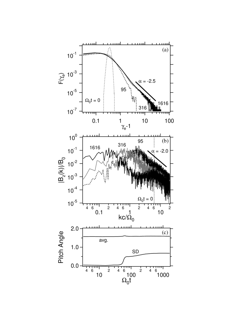
Figure 2: Electron energy distribution functions at various times.

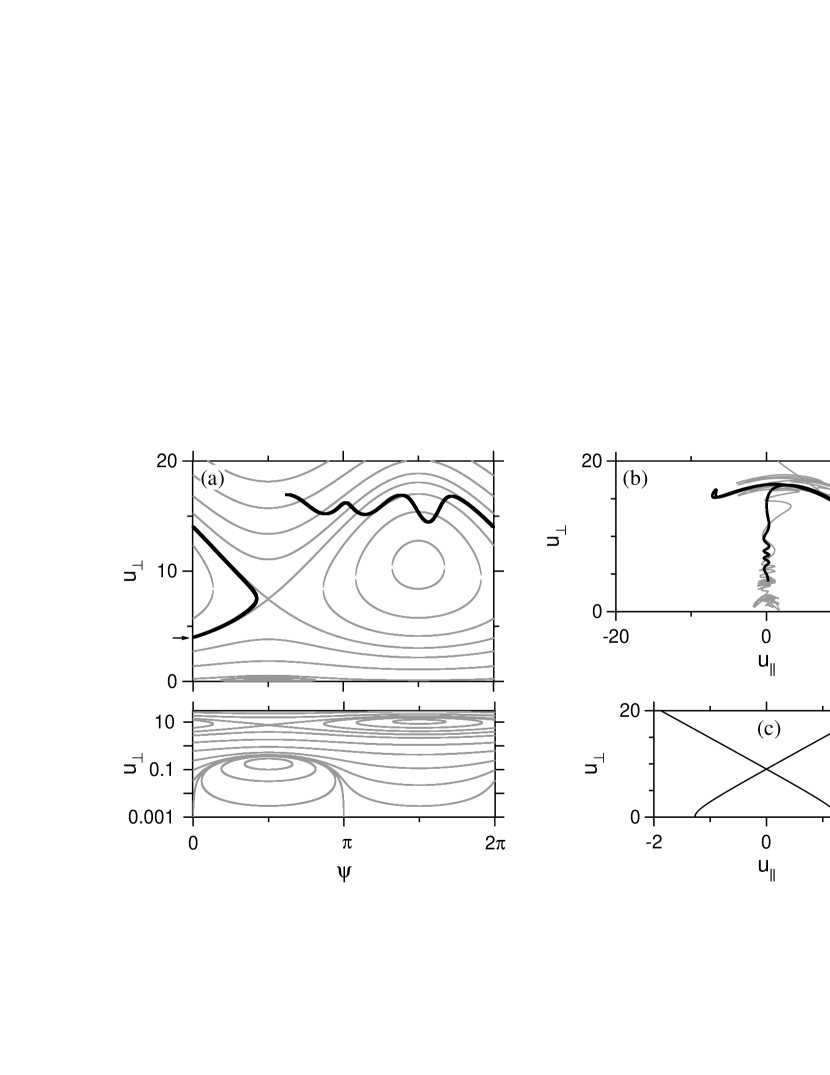
Figure 5: Electron trajectories in (a) $u_{\perp}-\psi$, (b) $u_{\perp}-u_{\parallel}$ phase space, and (c) linear resonance conditions of wave-particle interactions in relativistic (solid line) and nonrelativistic (dashed line) plamsas. Solutions of eq.(19) are plotted as gray lines in (a). In (b) a gray line denotes a trajectory of the electron shown in Fig.3. A numerical solution of eqs.(5) - (8) for $\Omega_{w}/\Omega_{0}=1,kc/|\Omega_{0}|=0.65$, and $\omega/|\Omega_{0}|=0.11$ is indicated as black lines in (a) and (b).

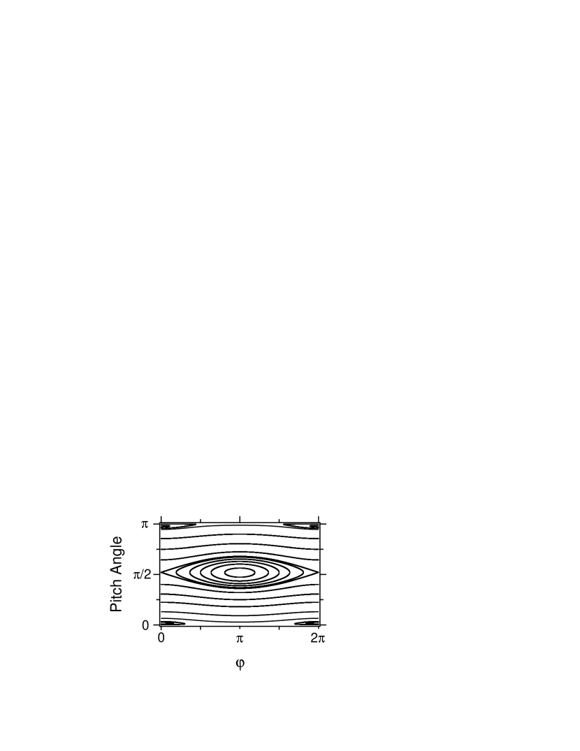
Figure 9: Trajectories of relativistic electrons interacting with the monochromatic circularly polarized parent wave. $B_{w}/B_{0}=1$, $kc/\Omega_{0}=6.21$, and $u=0.64$ are assumed.

References

- Krymsky (1977) Krymsky, G. F. 1977, Sov. Phys.-Dokl., 23, 327
- Axford et al. (1977) Axford, W., Leer, I. E., & Skadron, G. 1977, Proc. 15th Int. Cosmic Ray Conf. Plovdiv, 11, 132
- Bell (1978) Bell, A. R. 1978, MNRAS, 182, 147
- Blandford & Ostriker (1978) Blandford, R. D., & Ostriker, J. P. 1978, ApJ, 221, L29
- Drury (1983) Drury, L. O’C. 1983, Rep. Prog. Phys., 46, 973
- Lagage & Cesarsky (1983) Lagage, P. O., & Cesarsky, C. J. 1983, A&A, 125, 249
- Blandford & Eichler (1987) Blandford, R. D., & Eichler, D. 1987, Phys. Rep., 154, 1
- Jones & Ellison (1991) Jones, F. C., & Ellison, D. C. 1991, Space Sci. Rev., 58, 259
- Malkov & Drury (2001) Malkov, E., & Drury, L. O’C. 2001, Rep. Prog. Phys., 64, 429
- Duffy & Blundell (2005) Duffy, P., & Blundell, K. M. 2005, Plasma Phys. Control. Fusion, 47, B667
- de Wit et al. (1999) de Wit, T. D., Krasnosel’skikh, V. V., Dunlop, M., & Lühr, H. 1999, J. Geophys. Res., 104, 17,079, DOI:10.1029/1999JA900134
- Hada et al. (2003) Hada, T., Koga, D., & Yamamoto, E. 2003, Space Sci. Rev., 107, 463, DOI:10.1023/A:1025506124402
- Narita et al. (2006) Narita, Y., Glassmeier, K.-H., & Treumann, R. A. 2006, Phys. Rev. Lett., 97, id.191101, DOI:10.1103/PhysRevLett.97.191101
- Bruno & Carbone (2005) Bruno, R., & Carbone, V. 2005, Living Rev. Solar Phys., 24, http://www.livingreviews.org/lrsp-2005-4
- Kuramitsu & Hada (2008) Kuramitsu, Y., & Hada, T. 2008, Nonlin. Processes Geophys., 15, 265
- Kuramitsu & Hada (2000) Kuramitsu, Y., & Hada, T. 2000, Geophys. Res. Lett., 27, 629
- Spangler et al. (1997) Spangler, S. R., Leckband, J. A., & Cairns, I. 1997, Phys. Plasmas, 4, 846
- Spangler & Fuselier (1988) Spangler, S. R., & Fuselier, S. 1988, J. Geophys. Res., 93, 845
- Galeev & Oraevskii (1963) Galeev, A. A., & Oraevskii, V. N. 1963, Sov. Phys. Dokl., 7, 988
- Sagdeev & Galeev (1969) Sagdeev, R. Z., & Galeev, A. A. 1969, Nonlinear Plasma Theory, New York: Benjamin
- Kuramitsu & Krasnoselskikh (2005) Kuramitsu, Y., & Krasnoselskikh, V. 2005, A&A, 438, 391
- Chin & Wentzel (1972) Chin, Y. C., & Wentzel, D. G. 1972, Astrophys. Space Sci., 16, 465
- Wentzel (1974) Wentzel, D. G. 1974, A. Rev. Astr. Astrophys., 12, 71
- Skilling (1975a) Skilling, J. 1975a, MNRAS, 172, 557
- Skilling (1975b) Skilling, J. 1975b, MNRAS, 173, 245
- Skilling (1975c) Skilling, J. 1975c, MNRAS, 173, 255
- Matsukiyo & Hada (2003) Matsukiyo, S., & Hada, T. 2003, Phys. Rev. E, 67, id. 046406, DOI:10.1103/PhysRevE.67.046406
- Terasawa et al. (1986) Terasawa, T., Hoshino, M., Sakai, J-I., & Hada, T. 1986, J. Geophys. Res., 91, 4171
- Nariyuki & Hada (2005) Nariyuki, Y., & Hada, T. 2005, Earth, Planets, Space, 57, e9
- Nariyuki & Hada (2006) Nariyuki, Y., & Hada, T. 2006, Nonlin. Proc. Geophys., 13, 425
- Hada et al. (2004) Hada, T., Matsukiyo, S., & Muñoz, V. 2004, 12th Int’l Cong. Plasma Phys., 25-29 October 2004, Nice
- Shimada & Hoshino (2000) Shimada, N., & Hoshino, M. 2000, ApJ, 543, L67
- McClements et al. (2001) McClements, K. G., Dieckmann, M. E., Ynnerman, A., Chapman, S. C., Dendy, R. O. 2001, Phys. Rev. Lett., 87, 255002
- Hoshino & Shimada (2002) Hoshino, M., Shimada, N. 2002, ApJ, 572,880
- Dieckmann et al. (2004) Dieckmann, M. E., Eliasson, B., Shukla, P. K. 2004, ApJ, 617, 1361
- Dieckmann et al. (2005) Dieckmann, M. E., Eliasson, B., Parviainen, M., Shukla, P. K., Ynnerman, A. 2005, MNRAS, 367, 865
- Amano & Hoshino (2007) Amano, T, Hoshino, M. 2007, ApJ, 661, 190
- Tajima & Dawson (1979) Tajima, T., Dawson, J. M. 1979, Phys. Rev. Lett., 43, 267
- Katsouleas & Dawson (1983) Katsouleas, T, Dawson, J. M. 1983, IEEE Trans. Nucl. Sci., 30, 3241
- Lyubarsky (2006) Lyubarsky, Y 2006, ApJ, 652, 1297L
- Wykes et al. (2001a) Wykes, W. J., Chapman, S. C., Rowlands, G. 2001a, Planet. Space Sci., 49, 395
- Wykes et al. (2001b) Wykes, W. J., Chapman, S. C., Rowlands, G. 2001b, Phys. Plasmas, 8, 2953
- Hoshino (2008) Hoshino, M. 2008, ApJ, 672, 940
- Viñas & Goldstein (1991) Viñas, A. F., Goldstein, M. L. 1991, J. Plasma Phys., 46, 129
- Ghosh et al. (1993) Ghosh, S., Viñas, A. F., Goldstein, M. L. 1993, J. Geophy. Res., 98, 15561
- Ghosh et al. (1994) Ghosh, S., Viñas, A. F., Goldstein, M. L. 1994, J. Geophy. Res., 99, 19289
- Del Zanna et al. (2001) Del Zanna, L., Velli, M., Londrillo, P. 2001, A&A, 367, 705
- Amano & Hoshino (2008) Amano, T., Hoshino, M. 2008, ApJ, submitted
- Lucek & Bell (2000) Lucek, S. G., & Bell, A. R. 2000, MNRAS, 314, 65
- Bell & Lucek (2001) Bell, A. R., & Lucek, S. G. 2001, MNRAS, 321, 433
- Bell (2004) Bell, A. R. 2004, MNRAS, 353, 550
- Bell (2005) Bell, A. R. 2005, MNRAS, 358, 181