Reference Frames and the Physical Gravito-Electromagnetic Analogy

Abstract

The similarities between linearized gravity and electromagnetism are known since the early days of General Relativity. Using an exact approach based on tidal tensors, we show that such analogy holds only on very special conditions and depends crucially on the reference frame. This places restrictions on the validity of the “gravito-electromagnetic” equations commonly found in the literature.

1 Gravito-electromagnetic analogy based on tidal tensors

The topic of the gravito-electromagnetic analogies has a long story, with different analogies being unveiled throughout the years. Some are purely formal analogies, like the splitting of the Weyl tensor in electric and magnetic parts, e.g. [Maartens-Basset 1998]; but others (e.g [Damour et al. 1991, Costa-Herdeiro 2008, Jantzen et al. 1992, Natário 2007, Ruggiero-Tartaglia 2002]) stem from certain physical similarities between the gravitational and electromagnetic interactions. The linearized Einstein equations (see e.g. [Damour et al. 1991, Ruggiero-Tartaglia 2002, Ciufolini-Wheeler 1995]), in the harmonic gauge $\bar{h}_{\alpha\beta}^{\,\,\,\,\,\,,\beta}=0$, take the form $\square\bar{h}^{\alpha\beta}=-16\pi T^{\alpha\beta}/c^{4}$, similar to Maxwell equations in the Lorentz gauge: $\square A^{\beta}=-4\pi j^{\beta}/c$. That suggests an analogy between the trace reversed time components of the metric tensor $\bar{h}_{0\alpha}$ and the electromagnetic 4-potential $A_{\alpha}$. Defining the 3-vectors usually dubbed gravito-electromagnetic fields, the time components of these equations may be cast in a Maxwell-like form, e.g. eqs (16)-(22) of [Ruggiero-Tartaglia 2002]. Furthermore (on certain special conditions, see section 2) geodesics, precession and forces on gyroscopes are described in terms of these fields in a form similar to their electromagnetic counterparts, e.g. [Ruggiero-Tartaglia 2002], [Ciufolini-Wheeler 1995]. Such analogy may actually be cast in an exact form using the 3+1 splitting of spacetime (see [Jantzen et al. 1992, Natário 2007]).

These are analogies comparing physical quantities (electromagnetic forces) from one theory with inertial gravitational forces (i.e. fictitious forces, that can be gauged away by moving to a freely falling frame, due to the equivalence principle); it is clear that (non-spinning) test particles in a gravitational field move with zero acceleration $DU^{\alpha}/d\tau=0$; and that the spin 4-vector of a gyroscope undergoes Fermi-Walker transport $DS^{\alpha}/d\tau=S_{\sigma}U^{\alpha}DU^{\sigma}/d\tau$, with no real torques applied on it. In this sense the gravito-electromagnetic fields are pure coordinate artifacts, attached to the observer’s frame.

However, these approaches describe also (not through the “gravito-electromagnetic” fields themselves, but through their derivatives; and, again, under very special conditions) tidal effects, like the force applied on a gyroscope. And these are covariant effects, implying physical gravitational forces.

Herein we will discuss under which precise conditions a similarity between gravity and electromagnetism occurs (that is, under which conditions the physical analogy $\bar{h}_{0\mu}\leftrightarrow A_{\mu}$ holds, and Eqs. like (16)-(22) of [Ruggiero-Tartaglia 2002] have a physical content). For that we will make use of the tidal tensor formalism introduced in [Costa-Herdeiro 2008]. The advantage of this formalism is that, by contrast with the approaches mentioned above, it is based on quantities which can be covariantly defined in both theories — tidal forces (the only physical forces present in gravity) — which allows for a more transparent comparison between the electromagnetic (EM) and gravitational (GR) interactions.

Table 1: The gravito-electromagnetic analogy based on tidal tensors.

Electromagnetism		Gravity
Worldline deviation:		Geodesic deviation:
${\displaystyle\frac{D^{2}\delta x^{\alpha}}{d\tau^{2}}=\frac{q}{m}E_{\,\,\,\beta}^{\alpha}\delta x^{\beta}},\,\,\,E_{\,\,\,\beta}^{\alpha}\equiv F_{\ \mu;\beta}^{\alpha}U^{\mu}$	(1a)	${\displaystyle\frac{D^{2}\delta x^{\alpha}}{d\tau^{2}}=-\mathbb{E}_{\,\,\,\beta}^{\alpha}\delta x^{\beta}},\,\,\,\mathbb{E}_{\,\,\,\beta}^{\alpha}\equiv R_{\,\,\,\mu\beta\nu}^{\alpha}U^{\mu}U^{\nu}$	(1b)
Force on magnetic dipole:		Force on gyroscope:
${\displaystyle F_{EM}^{\beta}=\frac{q}{2m}B_{\alpha}^{\,\,\,\beta}S^{\alpha}},\,\,\,B_{\,\,\,\beta}^{\alpha}\equiv\star F_{\ \mu;\beta}^{\alpha}U^{\mu}$	(2a)	${\displaystyle F_{G}^{\beta}=-\mathbb{H}_{\alpha}^{\,\,\,\beta}S^{\alpha}},\,\,\,\mathbb{H}_{\,\,\,\beta}^{\alpha}\equiv\star R_{\,\,\,\mu\beta\nu}^{\alpha}U^{\mu}U^{\nu}$	(2b)
Maxwell Equations:		Eqs. Grav. Tidal Tensors:
$E_{\,\,\,\alpha}^{\alpha}=4\pi\rho_{c}$	(3a)	$\mathbb{E}_{\,\,\,\alpha}^{\alpha}=4\pi\left(2\rho_{m}+T_{\,\,\alpha}^{\alpha}\right)$	(3b)
$E_{[\alpha\beta]}=\frac{1}{2}F_{\alpha\beta;\gamma}U^{\gamma}$	(4a)	$\mathbb{E}_{[\alpha\beta]}=0$	(4b)
$B_{\,\,\,\alpha}^{\alpha}=0$	(5a)	$\mathbb{H}_{\,\,\,\alpha}^{\alpha}=0$	(5b)
$B_{[\alpha\beta]}=\frac{1}{2}\star F_{\alpha\beta;\gamma}U^{\gamma}-2\pi\epsilon_{\alpha\beta\sigma\gamma}j^{\sigma}U^{\gamma}$	(6a)	$\mathbb{H}_{[\alpha\beta]}=-4\pi\epsilon_{\alpha\beta\sigma\gamma}J^{\sigma}U^{\gamma}$	(6b)

$\rho_{c}=-j^{\alpha}U_{\alpha}$ and $j^{\alpha}$ are, respectively, the charge density and current 4-vector; $\rho_{m}=T_{\alpha\beta}U^{\alpha}U^{\beta}$ and $J^{\alpha}=-T_{\,\beta}^{\alpha}U^{\beta}$ are the mass/energy density and current (quantities measured by the observer of 4-velocity $U^{\alpha}$); $T_{\alpha\beta}\equiv$ energy-momentum tensor; $S^{\alpha}\equiv$ spin 4-vector; $\star\equiv$ Hodge dual. We use $\tilde{e}_{0123}=-1$.

The tidal tensor formalism unveils a new gravito-electromagnetic analogy, summarized in Table 1, based on exact and covariant equations. These equations make clear key differences, and under which conditions a similarity between the two interactions may occur.

Eqs. (1) are the worldline deviation equations yielding the relative acceleration of two neighboring particles (connected by the infinitesimal vector $\delta x^{\alpha}$) with the same 4-velocity $U^{\alpha}$ (and the same $q/m$ ratio, in the electromagnetic case). These equations manifest the physical analogy between electric tidal tensors: $\mathbb{E}_{\alpha\beta}\leftrightarrow E_{\alpha\beta}$.

Eq. (2a) yields the electromagnetic force exerted on a magnetic dipole moving with 4-velocity $U^{\alpha}$, and is the covariant generalization of the usual 3-D expression $\mathbf{F_{EM}}=\nabla(\mathbf{S}.\mathbf{B})q/2m$ (valid only in the dipole’s proper frame); Eq. (2b) is exactly the Papapetrou-Pirani equation for the gravitational force exerted on a spinning test particle. In both (2a) and (2b), Pirani’s supplementary condition $S_{\mu\nu}U^{\nu}=0$ is assumed (c.f. [Costa-Herdeiro 2009]). These equations manifest the physical analogy between magnetic tidal tensors: $B_{\alpha\beta}\leftrightarrow\mathbb{H}_{\alpha\beta}$.

Taking the traces and antisymmetric parts of the EM tidal tensors, one obtains Eqs. (3a)-(6a), which are explicitly covariant forms for each of Maxwell equations. Eqs. (3a) and (6a) are, respectively, the time and space projections of Maxwell equations $F_{\ \ \ ;\beta}^{\alpha\beta}=4\pi j^{\alpha}$; i.e., they are, respectively, covariant forms of $\nabla\cdot\mathbf{E}=4\pi\rho_{c}$ and $\nabla\times\mathbf{B}=\partial\mathbf{E}/\partial t+4\pi\mathbf{j}$; Eqs. (4a) and (5a) are the space and time projections of the electromagnetic Bianchi identity $\star F_{\ \ \ ;\beta}^{\alpha\beta}=0$; i.e., they are covariant forms for $\nabla\times\mathbf{E}=-\partial\mathbf{B}/\partial t$ and $\nabla\cdot\mathbf{B}=0$. These equations involve only tidal tensors and sources, which can be seen substituting the following decomposition (or its Hodge dual) in (4a) and (6a):

$$F_{\alpha\beta;\gamma}=2U_{[\alpha}E_{\beta]\gamma}+\epsilon_{\alpha\beta\mu\sigma}B_{\,\,\,\gamma}^{\mu}U^{\sigma}\ .$$ (1)

It is then straightforward to obtain the physical gravitational analogues of Maxwell equations: one just has to apply the same procedure to the gravitational tidal tensors, i.e., write the equations for their traces and antisymmetric parts (that is more easily done decomposing the Riemann tensor in terms of the Weyl tensor and source terms, see [Costa-Herdeiro 2007] sec. 2), which leads to Eqs. (3b) - (6b). Underlining the analogy with the situation in electromagnetism, Eqs. (3b) and (6b) turn out to be the time-time and and time-space projections of Einstein equations $R_{\mu\nu}=8\pi(T_{\mu\nu}-\frac{1}{2}g_{\mu\nu}T_{\,\,\,\alpha}^{\alpha})$, and Eqs. (4b) and (5b) the time-space and time-time projections of the algebraic Bianchi identities $\star R_{\ \ \ \gamma\beta}^{\gamma\alpha}=0$.

1.1 Gravity vs Electromagnetism

Charges — the gravitational analogue of $\rho_{c}$ is $2\rho_{m}+T_{\,\,\alpha}^{\alpha}$ ($\rho_{m}+3p$ for a perfect fluid) $\Rightarrow$ in gravity, pressure and all material stresses contribute as sources.

Ampere law — in stationary (in the observer’s rest frame) setups, $\star F_{\alpha\beta;\gamma}U^{\gamma}$ vanishes and equations (6a) and (6b) match up to a factor of 2 $\Rightarrow$ currents of mass/energy source gravitomagnetism like currents of charge source magnetism.

Symmetries of Tidal Tensors — The GR and EM tidal tensors do not generically exhibit the same symmetries, signaling fundamental differences between the two interactions. In the general case of fields that are time dependent in the observer’s rest frame (that is the case of an intrinsically non-stationary field, or an observer moving in a stationary field), the electric tidal tensor $E_{\alpha\beta}$ possesses an antisymmetric part, which is the covariant derivative of the Maxwell tensor along the observer’s worldline; there is also an antisymmetric contribution $\star F_{\alpha\beta;\gamma}U^{\gamma}$ to $B_{\alpha\beta}$. These terms consist of time projections of EM tidal tensors (cf. decomposition 1), and contain the laws of electromagnetic induction. The gravitational tidal tensors, by contrast, are symmetric (in vacuum, in the magnetic case) and spatial, manifesting the absence of analogous effects in gravity.

Gyroscope vs. magnetic dipole — According to Eqs. (2), both in the case of the magnetic dipole and in the case of the gyroscope, it is the magnetic tidal tensor, as seen by the test particle ($U^{\alpha}$ in Eqs. (2) is the gyroscope/dipole 4-velocity), that determines the force exerted upon it. Hence, from Eqs. (6), we see that the forces can be similar only if the fields are stationary (besides weak) in the gyroscope/dipole frame, i.e., when it is at “rest” in a stationary field. Eqs. (2) also tell us that in gravity the angular momentum $S$ plays the role of the magnetic moment $\mu=S(q/2m)$; the relative minus sign manifests that masses/charges of the same sign attract/repel one another in gravity/electromagnetism, as do charge/mass currents with parallel velocity.

2 Linearized Gravity

If the fields are stationary in the observer’s rest frame, the GR and EM tidal tensors have the same symmetries, which by itself does not mean a close similarity between the two interactions (note that despite the analogy in Table 1, EM tidal tensors are linear, whereas the GR ones are not). But in two special cases a matching between tidal tensors occurs: ultrastationary spacetimes (where the gravito-magnetic tidal tensor is linear, see [Costa-Herdeiro 2008] Sec. IV) and linearized gravitational perturbations, which is the case of interest for astronomical applications.

Consider an arbitrary electromagnetic field $A^{\alpha}=(\phi,\mathbf{A})$ and arbitrary perturbations around Minkowski spacetime in the form

$$ds^{2}=-c^{2}\left(1-2\frac{\Phi}{c^{2}}\right)dt^{2}-\frac{4}{c}\mathcal{A}_{j}dtdx^{j}+\left[\delta_{ij}+2\frac{\Theta_{ij}}{c^{2}}\right]dx^{i}dx^{j}\ .$$ (2)

Tidal effects. — The GR and EM tidal tensors from these setups will be in general very different, as is clear from equations (3-6), and as one may check from the explicit expressions in [Costa-Herdeiro 2008].

But if one considers time independent fields, and a static observer of 4-velocity $U^{\mu}=c\delta_{0}^{\mu}$, then the linearized gravitational tidal tensors match their electromagnetic counterparts identifying $(\phi,A^{i})\leftrightarrow(\Phi,\mathcal{A}^{i})$ (in expressions below colon represents partial derivatives; $\epsilon_{ijk}\equiv$ Levi Civita symbol):

$$\mathbb{E}_{ij}\simeq-\Phi_{,ij}\stackrel{{\scriptstyle\Phi\leftrightarrow\phi}}{{=}}E_{ij},\quad\mathbb{H}_{ij}\simeq\epsilon_{i}^{\,\,\,lk}\mathcal{A}_{k,lj}\stackrel{{\scriptstyle\mathcal{A}\leftrightarrow A}}{{=}}B_{ij}\ .$$ (3)

This suggests the physical analogy $(\phi,A^{i})\leftrightarrow(\Phi,\mathcal{A}^{i})$, and defining the “gravito-electro-magnetic fields” $\mathbf{E_{G}}=-\nabla\Phi$ and $\mathbf{B_{G}}=\nabla\times\bm{\mathcal{A}}$, in analogy with the electromagnetic fields $\mathbf{E}=-\nabla\phi,$ $\mathbf{B}=\nabla\times\mathbf{A}$. In terms of these fields we have $\mathbb{E}_{ij}\simeq(E_{G})_{i,j}$ and $\mathbb{H}_{ij}\simeq(B_{G})_{i,j}$, in analogy with the electromagnetic tidal tensors $E_{ij}=E_{i,j}$ and $B_{ij}=B_{i,j}$.

The matching (3) means that a gyroscope at rest (relative to the static observer) will feel a force $F_{G}^{\alpha}$ similar to the electromagnetic force $F_{EM}^{\alpha}$ on a magnetic dipole, which in this case take the very simple forms (time components are zero):

$$\mathbf{F_{EM}}=\frac{q}{2mc}\nabla(\mathbf{B}.\mathbf{S});\ \ \ \ \ F_{G}^{j}=-\frac{1}{c}\mathbb{H}^{ij}S_{i}\approx-\frac{1}{c}(B_{G})^{i,j}S_{i}\ \Leftrightarrow\ \mathbf{F_{G}}=-\frac{1}{c}\nabla(\mathbf{B_{G}}.\mathbf{S})\ .$$ (4)

Had we considered gyroscopes/dipoles with different 4-velocities, not only the expressions for the forces would be more complicated, but also the gravitational force would significantly differ from the electromagnetic one, as one may check comparing Eqs. (12) with (17)-(20) of [Costa-Herdeiro 2008]. This will be exemplified in section 2.1.

The matching (3) also means, by similar arguments, that the relative acceleration between two neighboring masses $D^{2}\delta x^{i}/d\tau^{2}=-\mathbb{E}^{ij}\delta x_{j}$ is similar to the relative acceleration between two charges (with the same $q/m$): $D^{2}\delta x^{i}/d\tau^{2}=E^{ij}\delta x_{j}(q/m)$, at the instant when the test particles have 4-velocity $U^{\alpha}=c\delta_{0}^{\alpha}$ (i.e., are at rest relative to the static observer $\mathcal{O}$).

Gyroscope precession. — The evolution of the spin vector of the gyroscope is given by the Fermi-Walker transport law, which, for a gyroscope at rest reads $DS^{i}/d\tau=0$; hence, we have, in the coordinate basis, Eq. (5a). The last term of Eq. (5a) vanishes if we express $\mathbf{S}$ in the local orthonormal tetrad $e^{\hat{\alpha}}$: $S^{i}=S^{\hat{i}}e_{\,\hat{i}}^{i}$, where to linear order $e_{\,\hat{i}}^{i}=\delta_{\ \hat{i}}^{i}-\Theta_{\ \ \hat{i}}^{i}/c^{2}$; in this fashion we obtain Eq. (5b), which is similar to the precession of a magnetic dipole in a magnetic field $d\mathbf{S}/dt=q\mathbf{S}\times\mathbf{B}/2mc$:

$$\frac{dS^{i}}{dt}=-c\Gamma_{0j}^{i}S^{j}=-\frac{1}{c}\left[(\mathbf{S}\times\mathbf{B_{G}})^{i}+\frac{1}{c}\frac{\partial\Theta_{\ }^{ij}}{\partial t}S_{j}\right]\ \ (a);\ \ \ \ \ \ \frac{dS^{\hat{i}}}{dt}=-\frac{1}{c}(\mathbf{S}\times\mathbf{B_{G}})^{\hat{i}}\ \ (b).$$ (5)

Thus, in the special case of gyroscope precession, the linear gravito-electromagnetic analogy holds even if the fields vary with time.

Geodesics. — The space part of the equation of geodesics $U_{\ ,\beta}^{\alpha}U^{\beta}=-\Gamma_{\beta\gamma}^{\alpha}U^{\beta}U^{\gamma}$ is given, to first order in the perturbations and in test particle’s velocity, by ($a^{i}\equiv d^{2}x^{i}/dt^{2})$:

$$\mathbf{a} = \nabla\Phi+\frac{2}{c}\frac{\partial\bm{\mathcal{A}}}{\partial t}-\frac{2}{c}\mathbf{v}\times(\nabla\times\bm{\mathcal{A}})-\frac{1}{c^{2}}\left[\frac{\partial\Phi}{\partial t}\mathbf{v}+2\frac{\partial\Theta_{\ j}^{i}}{\partial t}v^{j}\mathbf{e_{i}}\right]\ .$$ (6)

Comparing with the electromagnetic Lorentz force:

$$\mathbf{a}=\frac{q}{m}\left[-\nabla\phi-\frac{1}{c}\frac{\partial\mathbf{A}}{\partial t}+\frac{\mathbf{v}}{c}\times(\nabla\times\mathbf{A})\right]=\frac{q}{m}\left[\mathbf{E}+\frac{\mathbf{v}}{c}\times\mathbf{B}\right]\,,$$ (7)

these equations do not manifest, in general, a close analogy. Note that the last term of (6), which has no electromagnetic analogue, is, for the problem at hand (see next section), of the same order of magnitude as the second and third terms. But when one considers stationary fields, then (6) takes the form $\mathbf{a}=-\mathbf{E_{G}}-2\mathbf{v}\times\mathbf{B_{G}}/c$ analogous to (7).

Note the difference between this analogy and the one from the tidal effects considered above: in the case of the latter, the similarity occurs only when the test particle sees time independent fields (fields $\equiv$ derivatives of potentials/of metric perturbations); for geodesics, it is when the observer (not the test particle!) sees a time independent potential ($\phi$)/metric perturbations($\Phi,\Theta_{ij}$).

2.1 Translational vs. Rotational Mass Currents

The existence of a similarity between gravity and electromagnetism thus relies on the time dependence of the mass currents: if the currents are (nearly) stationary, for instance from a spinning celestial body, the gravitational field generated is analogous to a magnetic field; an example is the gravitomagnetic field due to the rotation of the Earth, detected on LAGEOS data by [Ciufolini et al.] (and which is also the subject of experimental scrutiny by the Gravity Probe B and the upcoming LARES missions). But when the currents seen by the observer vary with time — e.g. the ones resulting from translation of the celestial body, considered in [Soffel et al. 2008] — then the dynamics differ significantly.

Rotational Currents. — We will start by the well known analogy between the electromagnetic field of a spinning charge (charge $Q$, magnetic moment $\mu$) and the gravitational field (in the far region $r\rightarrow\infty$) of a rotating celestial body (mass $m$, angular momentum $J$), see Fig. 1

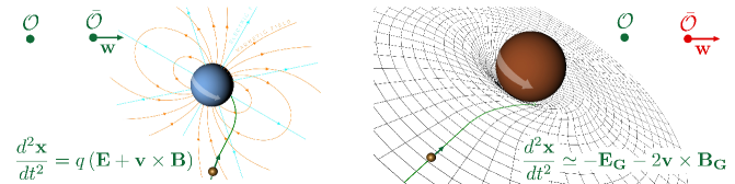
Figure 1: Spinning charge vs. spinning mass

The electromagnetic field of the spinning charge is described by the 4-potential $A^{\alpha}=(\phi,\mathbf{A})$, given by (8a). The spacetime around the spinning mass is asymptotically described by the linearized Kerr solution, obtained by putting in (2) the perturbations (8b) :

$$\phi=\frac{Q}{r}\ ,\ \ \ \mathbf{A}=\frac{1}{c}\frac{\bm{\mathbf{\mu}}\times\mathbf{r}}{r^{3}}\ \ \ (a);\ \ \ \ \ \ \Phi=\frac{M}{r}\ ,\ \ \ \bm{\mathcal{A}}=\frac{1}{c}\frac{\mathbf{J}\times\mathbf{r}}{r^{3}}\ ,\ \ \Theta_{ij}=\Phi\delta_{ij}\ \ \ (b).\ \ \$$ (8)

For the observer at rest $\mathcal{O}$ the gravitational tidal tensors asymptotically match the electromagnetic ones, identifying the appropriate parameters:

$$\mathbb{E}_{ij}\simeq\frac{M}{r^{3}}\delta_{ij}-\frac{3Mr_{i}r_{j}}{r^{5}}\stackrel{{\scriptstyle M\leftrightarrow Q}}{{=}}E_{ij};\ \ \ \ \mathbb{H}_{ij}\simeq\frac{3}{c}\left[\frac{(\mathbf{r}.\mathbf{J})}{r^{5}}\delta_{ij}+2\frac{r_{(i}J_{j)}}{r^{5}}-5\frac{(\mathbf{r}.\mathbf{J})r_{i}r_{j}}{r^{7}}\right]\stackrel{{\scriptstyle J\leftrightarrow\mu}}{{=}}B_{ij}$$

(all the time components are zero for this observer). This means that $\mathcal{O}$ will find a similarity between physical (i.e., tidal) gravitational forces and their electromagnetic counterparts: the gravitational force $F_{G}^{i}=-\mathbb{H}^{ji}S_{j}/c$ exerted on a gyroscope carried by $\mathcal{O}$ is similar to the force $F_{EM}^{i}=qB^{ji}S_{j}/2mc$ on a magnetic dipole; and the worldline deviation $D^{2}\delta x^{i}/d\tau^{2}=-\mathbb{E}^{ij}\delta x_{i}$ of two masses dropped from rest is similar to the deviation between two charged particles with the same $q/m$.

Moreover, observer $\mathcal{O}$ will see test particles moving on geodesics described by equations analogous to the electromagnetic Lorentz force (see Fig. 1).

Translational Currents. — For the observer $\bar{\mathcal{O}}$ moving with velocity $\mathbf{w}$ relative to the mass/charge of Fig. 1, however, the electromagnetic and gravitational interactions will look significantly different. For simplicity we will specialize here to the case where $\mathbf{J}=\bm{\mu}=0$, so that the mass/charge currents seen by $\bar{\mathcal{O}}$ arise solely from translation. To obtain the electromagnetic 4-potential $A^{\bar{\alpha}}$ in the frame $\bar{\mathcal{O}}$, we apply the boost $A^{\bar{\alpha}}=\Lambda_{\ \alpha}^{\bar{\alpha}}A^{\alpha}=(\bar{\phi},\bar{\mathbf{A}})$, where $\Lambda_{\ \alpha}^{\bar{\alpha}}\equiv\partial\bar{x}^{\bar{\alpha}}/\partial x^{\alpha}$, using the expansion of Lorentz transformation (as done in e.g. [Will-Nordtvedt 1972]):

$$t=\bar{t}\left(1+\frac{w^{2}}{2c^{2}}+\frac{3w^{4}}{8c^{4}}\right)+\left(1+\frac{w^{2}}{2c^{2}}\right)\frac{\mathbf{\bar{x}}.\mathbf{w}}{c^{2}};\ \ \ \ \mathbf{x}=\mathbf{\bar{x}}+\frac{1}{2c^{2}}(\bar{\mathbf{x}}.\mathbf{w})\mathbf{w}+\left(1+\frac{w^{2}}{2c^{2}}\right)\mathbf{w}\bar{t}\ ,$$ (9)

yielding, to order $c^{-2}$, $A^{\bar{\alpha}}=(\bar{\phi},\mathbf{\bar{A}})$, with $\bar{\phi}=Q(1+w^{2}/2c^{2})/r$ and $\mathbf{\bar{A}}=-Q\mathbf{w}/rc$. To obtain $A^{\bar{\alpha}}$ in the coordinates ($\bar{x}^{i},\bar{t}$) of $\bar{\mathcal{O}}$, we must also express $r$ (which denotes the distance between the source and the point of observation, in the frame $\mathcal{O}$) in terms of $R\equiv|\mathbf{\bar{r}}+\mathbf{w}\bar{t}|$, i.e., the distance between the source and the point of observation in the frame $\bar{\mathcal{O}}$. Using transformation (9), we obtain: $r^{-1}=R^{-1}[1-(\mathbf{w}.\mathbf{R})^{2}/(2R^{2}c^{2})]$, and finally the electromagnetic potentials seen by $\bar{\mathcal{O}}$:

$$\bar{\phi}=\frac{Q}{R}\left(1+\frac{w^{2}}{2c^{2}}-\frac{(\mathbf{w}.\mathbf{R})^{2}}{4R^{2}c^{2}}\right);\ \ \ \ \ \ \mathbf{\bar{A}}=-\frac{1}{c}\frac{Q}{R}\mathbf{w}\ .$$ (10)

The metric of the spacetime around a point mass, in the coordinates of $\bar{\mathcal{O}}$, is also obtained using transformation (9), which is accurate to Post Newtonian order, by an analogous procedure. First we apply the Lorentz boost $g_{\bar{\alpha}\bar{\beta}}=\Lambda_{\ \bar{\alpha}}^{\alpha}\Lambda_{\ \bar{\beta}}^{\beta}g_{\alpha\beta}$ to the metric (8) (with $\mathcal{A}=0$); then, expressing $r$ in terms of $R$, we finally obtain (note that, although we are not putting the bars therein, indices $\alpha=0,i$ in the following expressions refer to the coordinates of $\bar{\mathcal{O}}$):

$$g_{00} = -1+2\frac{M}{Rc^{2}}+\frac{4Mw^{2}}{Rc^{4}}-\frac{M(\mathbf{w}.\mathbf{R})^{2}}{c^{4}R^{3}}\equiv-1+\frac{2\bar{\Phi}}{c^{2}};\ \$$

$$\ g_{0i} = \frac{4Mw_{i}}{Rc^{3}}\equiv-\frac{2\bar{\mathcal{A}}_{i}}{c^{2}};\ \ \ \ \ \ \ \ \ \ g_{ij}=\left[1+2\frac{M}{Rc^{2}}\right]\delta_{ij}\equiv\left[1+2\frac{\bar{\Theta}}{c^{2}}\right]\delta_{ij}\ ,$$ (11)

where we retained terms up to $c^{-4}$ in $g_{00}$, up to $c^{-3}$ in $g_{i0}$ and $c^{-2}$ in $g_{ij}$, as usual in Post-Newtonian approximation. This matches, to linear order in $M$, Eqs. (5) of [Soffel et al. 2008] for the case of one single source; or e.g. Eqs. (11) of [Nordtvedt 1988] (in the case of the latter, an additional gauge choice, Eq. (19) of [Will-Nordtvedt 1972], was made). The metric (11), like the electromagnetic potential (10), is now time dependent, since $\mathbf{R}(\bar{t})=\mathbf{\bar{r}}+\mathbf{w}\bar{t}$.

The gravitational tidal tensors seen by $\bar{\mathcal{O}}$ are ($\mathbb{E}_{\alpha 0}=\mathbb{E}_{0\alpha}=\mathbb{H}_{\alpha 0}=\mathbb{H}_{0\alpha}=0$):

$$\mathbb{E}_{ij} = -\bar{\Phi}_{,ij}-\frac{2}{c}\frac{\partial}{\partial\bar{t}}\bar{\mathcal{A}}_{(i,j)}-\frac{1}{c^{2}}\frac{\partial^{2}}{\partial\bar{t}^{2}}\bar{\Theta}\delta_{ij}$$ (12)

$$= \frac{M\delta_{ij}}{R^{3}}\left[1+\frac{3w^{2}}{c^{2}}-\frac{9}{2}\frac{(\mathbf{R}.\mathbf{w})^{2}}{c^{2}R^{2}}\right]-\frac{3MR_{i}R_{j}}{R^{5}}\left[1+\frac{2w^{2}}{c^{2}}-\frac{5(\mathbf{R}.\mathbf{w})^{2}}{2c^{2}R^{2}}\right]$$

$$-\frac{3Mw_{i}w_{j}}{c^{2}R^{3}}+\frac{6Mw_{(i}R_{j)}(\mathbf{R}.\mathbf{w})}{c^{2}R^{5}};$$

$$\mathbb{H}_{ij} = \epsilon_{i}^{\,\,\,lk}\bar{\mathcal{A}}_{k,lj}-\frac{1}{c}\epsilon_{ij}^{\ \ l}\frac{\partial\bar{\Theta}_{,l}}{\partial\bar{t}}\ =\frac{M}{cR^{3}}\left[3\epsilon_{ij}^{\ \ k}w_{k}-\frac{3}{R^{2}}(\mathbf{R}.\mathbf{w})\epsilon_{ij}^{\ \ k}R_{k}-\frac{6}{R^{2}}(\mathbf{R}\times\mathbf{w})_{i}R_{j}\right],$$ (13)

which significantly differ from the electromagnetic ones ($E_{0\alpha}=B_{0\alpha}=0$):

$$E_{ij} = -\bar{\phi}_{,ij}-\frac{1}{c}\frac{\partial}{\partial\bar{t}}\bar{A}_{i;j}\ =\ E_{i,j}$$ (14)

$$= \frac{Q\delta_{ij}}{R^{3}}\left[1+\frac{w^{2}}{2c^{2}}-\frac{3}{4}\frac{(\mathbf{R}.\mathbf{w})^{2}}{c^{2}R^{2}}\right]-\frac{3QR_{i}R_{j}}{R^{5}}\left[1+\frac{w^{2}}{2c^{2}}-\frac{5(\mathbf{R}.\mathbf{w})^{2}}{4c^{2}R^{2}}\right]$$

$$-\frac{Qw_{i}w_{j}}{2c^{2}R^{3}}+\frac{3Qw_{[i}R_{j]}(\mathbf{R}.\mathbf{w})}{c^{2}R^{5}};$$

$$E_{i0} = -\frac{1}{c}\frac{\partial}{\partial\bar{t}}\bar{\phi}_{;i}-\frac{1}{c^{2}}\frac{\partial^{2}\bar{A}_{i}}{\partial\bar{t}^{2}}\ \equiv\frac{1}{c}\ \frac{\partial E_{i}}{\partial\bar{t}}\ =\ \frac{Q}{cR^{3}}\left[w_{i}-\frac{3(\mathbf{R}.\mathbf{w})R_{i}}{R^{2}}\right];$$ (15)

$$B_{ij} = \epsilon_{i}^{\ lm}\bar{A}_{m;lj}\ \equiv\ B_{i,j}=\frac{Q}{cR^{3}}\left[\epsilon_{ij}^{\ \ k}w_{k}-\frac{3}{R^{2}}(\mathbf{R}\times\mathbf{w})_{i}R_{j}\right];$$ (16)

$$B_{i0}\ = \frac{1}{c}\frac{\partial B_{i}}{\partial\bar{t}}=-\ \frac{3Q}{c^{2}R^{5}}(\mathbf{R}.\mathbf{w})(\mathbf{R}\times\mathbf{w})_{i}\ .$$ (17)

Note in particular that, unlike their gravitational counterparts, $E_{\alpha\beta}$ and $B_{\alpha\beta}$ are not symmetric, and have non-zero time components. The antisymmetric parts $E_{[ij]}=E_{[i,j]}$ and $B_{[ij]}=B_{[i,j]}$ above are (vacuum) Maxwell equations $\nabla\times\mathbf{E}=-(1/c)\partial\mathbf{B}/\partial t$ and $\nabla\times\mathbf{B}=(1/c)\partial\mathbf{E}/\partial t$, implying that a time varying electric/magnetic field endows the magnetic/electric tidal tensor with an antisymmetric part. For instance, a time varying electric field will always induce a force on a magnetic dipole. The fact that $\mathbb{E}_{\alpha\beta}$ and $\mathbb{H}_{\alpha\beta}$ are symmetric reflects the absence of analogous gravitational effects. The time component $B_{i0}$ means that the force on a magnetic dipole (magnetic moment $\mu=q/2m$) will have a time component $(F_{EM})_{0}=(1/c)\bm{\mu}.\partial\mathbf{B}/\partial t$, which (see [Costa-Herdeiro 2009] sec. 1.2) is minus the power transferred to the dipole by Faraday’s law of induction (and is reflected in the variation of the dipole’s proper mass $m=-P^{\alpha}U_{\alpha}/c^{2}$). Again, this is an effect which has no gravitational counterpart: $\mathbb{H}_{\alpha 0}=\mathbb{H}_{0\alpha}=0$, thus $(F_{G})_{0}=0$, and the proper mass of the gyroscope is a constant of the motion.

The space part of the geodesic equation for a test particle of velocity $\mathbf{v}$ is:

$$\mathbf{a} = \nabla\bar{\Phi}+\frac{2}{c}\frac{\partial\bm{\bar{\mathcal{A}}}}{\partial\bar{t}}-2\mathbf{v}\times(\nabla\times\bm{\bar{\mathcal{A}}})-\frac{3}{c^{2}}\frac{\partial}{\partial\bar{t}}\left(\frac{M}{R}\right)\mathbf{v}$$

$$= -\frac{M}{R^{3}}\left[1+\frac{2w^{2}}{c^{2}}-\frac{3(\mathbf{R}.\mathbf{w})^{2}}{2c^{2}R^{2}}\right]\mathbf{R}+\frac{3M(\mathbf{R}.\mathbf{w})}{c^{2}R^{3}}\mathbf{w}-\frac{4M}{c^{2}R^{3}}\mathbf{v}\times(\mathbf{R}\times\mathbf{w})+\frac{3}{c^{2}}\frac{M}{R^{3}}(\mathbf{R}.\mathbf{w})\mathbf{v}\ ,$$

which matches equation (10) of [Soffel et al. 2008], or (7) of [Nordtvedt 1973], again, in the special case of only one source, and keeping therein only linear terms in the perturbations and test particle’s velocity $\mathbf{v}$.

Comparing with its electromagnetic counterpart

$$\left(\frac{m}{q}\right)\mathbf{a}=\mathbf{E}+\frac{\mathbf{v}}{c}\times\mathbf{B}=\frac{Q}{R^{3}}\left[1+\frac{w^{2}}{2c^{2}}-\frac{3(\mathbf{R}.\mathbf{w})^{2}}{4c^{2}R^{2}}\right]\mathbf{R}-\frac{1}{2}\frac{Q(\mathbf{R}.\mathbf{w})}{c^{2}R^{3}}\mathbf{w}+\frac{Q}{c^{2}R^{3}}\mathbf{v}\times(\mathbf{R}\times\mathbf{w})$$

we find them similar to a certain degree (up to some factors), except for the last term of (2.1). That term signals a difference between the two interactions, because it means that there is a velocity dependent acceleration which is parallel to the velocity; that is in contrast with the situation in electromagnetism, where the velocity dependent accelerations arise from magnetic forces, and are thus always perpendicular to $\mathbf{v}$.

As expected from Eqs. (5) (and by contrast with the other effects), the precession of a gyroscope carried by $\bar{\mathcal{O}}$, Eq. (19b) takes a form analogous to the precession of a magnetic dipole, Eq. (19a), if we express $\mathbf{S}$ in the local orthonormal tetrad $e^{\hat{i}}$, non rotating relative to the inertial observer at infinity, such that $S^{i}=(1-M/R)S^{\hat{i}}$:

$$\frac{d\mathbf{S}}{d\bar{t}}=\frac{q}{2m}\frac{Q}{c^{2}R^{3}}\left[\mathbf{S}\times(\mathbf{R}\times\mathbf{w})\right]\ \ (a);\ \ \ \ \ \ \frac{dS^{\hat{i}}}{d\bar{t}}=\frac{2M}{c^{2}R^{3}}\left[(\mathbf{R}\times\mathbf{w})\times\mathbf{S}\right]^{\hat{i}}\ \ (b)\ .$$ (19)

If instead of the gyroscope comoving with observer $\bar{\mathcal{O}}$ (with constant velocity $\mathbf{w}$), we had considered a gyroscope moving in a circular orbit, then an additional term would arise in analogy with Thomas precession for the magnetic dipole; for a circular geodesic that term amounts to $-1/4$ of expression (19b), and we would obtain the well known equation for geodetic precession (e.g. [Ciufolini-Wheeler 1995]).

3 Conclusion

We conclude our paper by discussing some of the implications of our conclusions in the approaches usually found in literature. In the framework of linearized theory, e.g. [Ruggiero-Tartaglia 2002, Ciufolini-Wheeler 1995], Einstein equations are often written in a Maxwell-like form; likewise, geodesics, precession and gravitational force on a spinning test particle are cast (in terms of 3-vectors defined in analogy with the electromagnetic fields $\mathbf{E}$ and $\mathbf{B}$) in a form similar to, respectively, the Lorentz force on a charged particle, the precession and the force on a magnetic dipole.

We have concluded that the actual physical similarities between gravity and electromagnetism (on which the physical content of such approaches relies) occur only on very special conditions. For tidal effects, like the forces on a gyroscopes/dipoles, the analogy manifest in Eqs. (4) holds only when the test particle sees time independent fields. In the example of analogous systems considered in section 2.1, this means that the center of mass of the gyroscope/dipole must not move relative to the central body. In the case of the analogy between the equation of geodesics and the Lorentz force law (see Fig. 1), as manifest in equation (6), it is in the potentials/metric perturbations, as seen by the observer (not the test particle!), that the time independence is required. The latter condition is not as restrictive as the one of the tidal effects: consider for instance observers moving in circular orbits around a static mass/charge; such observers see an unchanging spacetime, and unchanging electromagnetic potentials, so, for them, the equation of geodesics and Lorentz force take similar forms (such analogy may actually be cast in an exact form, see [Natário 2007, Jantzen et al. 1992]). However, those observers see a time-varying electric field $\mathbf{E}$ (constant in magnitude, but varying in direction), which, by means of equations (4) and (6), implies that the tidal tensors are not similar to the gravitational ones.

Finally, as a consequence of this analysis, a distinction, from the point of view of the analogy with electrodynamics, between effects related to (stationary) rotational mass currents, and those arising from translational mass currents, becomes clear: albeit in the literature both are dubbed “gravitomagnetism”, one must note that, while the former are clearly analogous to magnetism, in the case of the latter the analogy is not so close.

Acknowledgments

We thank the anonymous referee for very useful comments and suggestions.

References

- [Maartens-Basset 1998] Maartens R., Basset B. 1998, Class. Q. Grav., 15, 705 [arXiv:gr-qc/9704059]
- [Damour et al. 1991] Damour T., Soffel M. , Xu C. . 1991, Phys. Rev. D., 43, 3273
- [Ruggiero-Tartaglia 2002] Ruggiero, M., & Tartaglia, A. 2002, Nuovo Cim., 117B 743 [arXiv:gr-qc/0207065].
- [Costa-Herdeiro 2008] Costa, L. Filipe O., & Herdeiro, Carlos A. R. 2008, Phys. Rev. D, 78, 024021
- [Costa-Herdeiro 2007] Costa, L. Filipe, & Herdeiro, Carlos A. R. 2007 [arXiv:gr-qc/0612140]
- [Costa-Herdeiro 2009] Costa, L. Filipe O., & Herdeiro, Carlos A. R. 2009, Int. J. Mod. Phys. A, 24, 1695
- [Ciufolini et al.] Ciufolini I., Pavlis E. 2004, Nature 431, 958; Ciufolini I., Pavlis E., Peron R., New Astron. 11, 527-550 (2006). The measurement of the Lense-Thirring effect is expected to be improved to an accuracy of a few percent by the upcoming LARES mission: http://lares.diaa.uniroma1.it/
- [Ciufolini-Wheeler 1995] Ciufolini I., Wheeler J. 1995, Gravitation and Inertia (Princeton Univ. Press)
- [Soffel et al. 2008] Soffel M., Klioner S., Muller J., Biskupek L. 2008, Phys. Rev. D, 78, 024033
- [Jantzen et al. 1992] Jantzen R., Carini P., Bini D. 1992, Ann. Phys., 215, 1 [arXiv:gr-qc/0106043].
- [Natário 2007] Natário J. 2007, Gen. Rel. Grav., 39, 1477 [arXiv:gr-qc/0701067].
- [Nordtvedt 1973] Nordtvedt K. 1973, Phys. Rev. D, 7, 2347
- [Will-Nordtvedt 1972] Will C., Nordtvedt K. 1972, APJ, 177, 757
- [Nordtvedt 1988] Nordtvedt K. 1988, Int. J. Theoretical Physics, 27, 2347