IPhT-t09/150

We show how the formulation of the matrix models as conformal field theories on a Riemann surfaces can be used to compute the genus expansion of the observables. Here we consider the simplest example of the hermitian matrix model, where the classical solution is described by a hyperelliptic Riemann surface. To each branch point of the Riemann surface we associate an operator which represents a twist field dressed by the modes of the twisted boson. The partition function of the matrix model is computed as a correlation function of such dressed twist fields. The perturbative construction of the dressing operators yields a set of Feynman rules for the genus expansion, which involve vertices, propagators and tadpoles. The vertices are universal, the propagators and the tadpoles depend on the the Riemann surface. As a demonstration we evaluate the genus-two free energy using the Feynman rules.

1 Introduction

In this paper, which is a continuation of [1], we formulate the $1/N$ expansion of $U(N)$ invariant matrix integrals as the quasiclassical expansion in conformal field theories on Riemann surfaces. Our basic example will be the hermitian matrix model defined by the partition function

$${\cal Z}_{N}[V] = \int d{\bf M}\,e^{-{\rm tr\,}V({\bf M})}$$ (1.1)

$$\sim \int\limits_{\cal C}\prod_{i=1}^{N}dz_{i}\ e^{-V(z_{i})}\ \prod_{i<j}(z_{i}-z_{j})^{2}.$$

Here $z_{1},\dots,z_{N}$ are the eigenvalues of the matrix variable ${\bf M}$ and

$$V(z)=-\sum_{n=0}^{\infty}t_{n}z^{n}\,$$ (1.2)

is a confining potential. For the hermitian matrix integral the contour of integration goes along the real axis. Then the integral is convergent if the potential becomes infinitely large when $z\to\pm\infty$. If this is not the case, the integral can be made convergent by deforming the contour of integration.

The $1/N$ expansion of the free energy ${\cal F}_{N}[V]=\ln{\cal Z}_{N}[V]$ is of the form

$${\cal F}_{N}[V]=\sum_{g=0}^{\infty}N^{2-2g}{\cal F}^{(g)}[V/N]+\ {\rm nonperturbative\ terms},$$ (1.3)

where the term ${\cal F}^{(g)}$ counts the number of genus $g$ fat Feynman graphs. The leading, genus zero, term can be obtained by evaluating the saddle point eigenvalue distribution [2]. In this approximation the eigenvalues can be considered as a continuous charged liquid defined by the spectral density

$$\rho(z)=\lim_{N\to\infty}{1\over N}\sum_{i=1}^{N}\delta(z-z_{i}).$$ (1.4)

The collective field theory for the spectral density (1.4) is ill defined at small distances and cannot be used to compute the higher terms of the quasiclassical expansion. This can be done by solving the Ward identities for the integral (1.1), known also as loop equations. An improved iterative scheme for calculating the higher genus observables, known as method of moments, was set up by Ambjorn, Chekhov, Kristjansen and Makeenko [3]. More recently, Eynard [4] formulated the recursion procedure for solving the loop equations in an elegant graphical scheme.

The form of the loop equations suggests that there is a local field theory hidden behind. Indeed, the loop equations can be formulated as Virasoro constraints for the bosonic field

$$\phi(z)=\sqrt{2}\sum_{i=1}^{N}\log\left(z-z_{i}\right)-{1\over\sqrt{2}}V(z)\,.$$ (1.5)

Therefore the theory in question must be a two-dimensional chiral CFT. An important feature of this CFT is that the bosonic field develops a large classical expectation value $\phi_{c}(z)$. The classical current $J_{c}=\partial_{z}\phi_{c}$ satisfies a quadratic equation, the classical Virasoro constraint, whose solution defines for a general potential a hyperelliptic Riemann surface with branch points $a_{1},\dots,a_{2p}$ placed on the real axis. The set of branch cuts along the segments $[a_{1},a_{2}],\dots,[a_{2p-1},a_{2p}]$ coincide with the support of the classical spectral density. Each branch cut is associated with a local minimum of the potential and is characterized by the filling number $N_{j}$, equal to the number of the eigenvalues trapped around this minimum.

In the chiral CFT the branch points of the Riemann surface can be thought of as the result of applying twist operators to the $sl(2)$ invariant vacuum. The twist operators are however not conformal invariant. In particular the translations change the positions of the branch points. In [1] we claimed that in order to satisfy the conformal Ward identity the twist operators should be dressed by the modes of the twisted boson. The dressed twist operators were called in [1] star operators because of the analogy with the star operators introduced by G. Moore in [5]. We should stress here that the star operators in [1] and in [5] are different objects.

The problem of computing the genus expansion of the of the observables is thus reduced to the perturbative construction of the operators dressing the twist fields. Such dressing operator represents a formal series expansion in the modes of the twisted boson. The coefficients of the expansion are related to the correlation functions in the Kontsevich model. In this sense the proposal made in [1] allows to decompose the hermitian matrix model with an arbitrary potential into $2p$ Kontsevich models coupled through the modes of a gaussian field on the hyperelliptic surface. Similar decomposition formulas for the hermitian matrix model were suggested in [6, 7, 8].

The aim of this paper is to present the details of the construction of the dressed twist operators and to set up the Feynman diagram technique for calculating the free energy and the expectation values in all orders on $1/N$.

The paper is organized as follows. In Section 2 we remind the Fock space representation of the integral (1.1) in terms of a chiral bosonic field $\phi(z)$ with Liouville-like interaction given in [1] and derive the loop equations from the conformal Ward identity. This Section helps to make the presentation self-consistent and can be skipped by the reader who is familiar with the loop equations. In 3 we give the representation of the leading and the subleading orders of the free energy in terms of the correlation function of $2p$ twist operators. In Section 4 we give the explicit prescription for dressing the twist operators and set up the Feynman rules for computing all orders of the genus expansion. This Feynman diagram technique is different than the diagram technique in [4]. In Section 5 we compute, using the Feynman rules, the genus two free energy and compare with the result of [3].

2 The matrix model as a chiral CFT

2.1 From Coulomb gas to compactified chiral boson

The Coulomb gas integral (1.1) can be represented as a Fock space expectation value in a theory of a Liouville-like chiral CFT with the wrong sign of the kinetic term. Introduce the holomorphic scalar field $\phi(z)$ with mode expansion at $z=\infty$

$$\phi(z) = \hat{q}+J_{0}\ln z-\sum_{n\neq 0}{J_{n}\over n}z^{-n}\ ,\quad[J_{n},J_{m}]=n\,\delta_{n+m,0},\quad[J_{0},\hat{q}]=1\,,$$ (2.1)

and left and right Fock vacua defined by

$$\langle 0|J_{0}=\hat{q}|0\rangle=0,\quad\langle 0|J_{-n}=J_{n}|0\rangle=0\quad(n\geq 1).$$ (2.2)

The field has operator product expansion

$$\phi(z)\,\phi(z^{\prime})\sim\ln(z-z^{\prime})\,$$ (2.3)

and give a representation of the $\hat{s}u(2)$ current algebra:

$$J={\textstyle{1\over\sqrt{2}}}\ \partial\phi(z),\quad J_{\pm}=:e^{\pm\sqrt{2}\phi}:\,.$$ (2.4)

Then the partition function (1.1) is given by the scalar product

$${\cal Z}_{N}=\langle N|e^{J[V]}\ e^{Q_{+}}|0\rangle,$$ (2.5)

where

$$J[V] = -\oint\limits_{\infty}{dz\over 2\pi i}V(z)J(z)=\sum_{n\geq 0}t_{n}\,J_{n}\,,$$ (2.6)

$$Q_{+} = \int_{-\infty}^{\infty}dz\ J_{+}(z)$$ (2.7)

and $\langle N|$ is the charged left vacuum state

$$\langle N|=\langle 0|e^{\sqrt{2}N\hat{q}}\,.$$ (2.8)

The operator $e^{Q_{+}}$ generates screening charges, the operator $e^{J[V]}$ produces the measure $e^{-V(z)}$ for each charge, and the left vacuum $\langle N|$ projects onto the sector with exactly $N$ screening charges. Similar Fock space representations of the eigenvalue integral have been proposed in [9, 10, 11].

The currents $J,J+$ and $J_{-}$ are invariant under the discrete translations of of the field $\phi$:

$$\phi\to\phi+i{\pi}{\sqrt{2}}.$$ (2.9)

Therefore the the field $\phi$ can be compactified at the self-dual radius $R_{\rm s.d.}=1/\sqrt{2}$. Furthermore, the transformation

$$\phi\to-\phi$$ (2.10)

is an automorphism of the current algebra. The geometrical meaning of the symmetry (2.10) will become clear when we consider the quasiclassical limit of the bosonic field.

The correlation functions of in the matrix model are obtained through the identification

$$\phi(z)=\sqrt{2}\ {\rm tr\,}\log\left(z-{\bf M}\right)-{1\over\sqrt{2}}V(z)\,$$ (2.11)

or, in terms of the $\hat{su}(2)$ currents,

$$J(z)={\rm tr\,}{1\over z-{\bf M}}-{\textstyle{1\over 2}}V^{\prime}(z)\,,\quad J_{\pm}(z)=e^{\mp V(z)}[\det(z-{\bf M})]^{\pm 2}.$$ (2.12)

2.2 Conformal Ward identity

To prove that the theory is conformal invariant we have to demonstrate that the energy-momentum tensor

$$T(z)={\textstyle{1\over 2}}:\partial\phi(z)\partial\phi(z):\,=\sum_{n}L_{n}z^{-n-2}$$ (2.13)

commutes with the screening operator $Q_{+}$. Indeed, for any $n\geq-1$ we have

$$[L_{n},Q_{+}]=\int_{-\infty}^{\infty}dz[L_{n},J_{+}(z)]=\int_{-\infty}^{\infty}dz\,{d\over dz}\Big{(}z^{n+1}J_{+}(z)\Big{)}.$$ (2.14)

Since our potential diverges at infinity, the boundary terms vanish and the result is zero for all $n\geq-1$. As a consequence, the expectation value

$$\left\langle\,T(z)\,\right\rangle\stackrel{{\scriptstyle\text{def}}}{{=}}\langle N|e^{J[V]}\ T(z)\,e^{Q_{+}}|0\rangle\,$$ (2.15)

is regular for $z\neq\infty$. This condition can be written as a contour integral which projects to the positive part of the Laurent expansion of $T(x)$:

$$\oint\limits_{\infty}{dz^{\prime}\over 2\pi i}\Big{\langle}{T(z)-T(z^{\prime})\over z-z^{\prime}}\Big{\rangle}=0.$$ (2.16)

The conformal Ward identity (2.16) is translated into a set of differential Virasoro constraints on the partition function using the representation of the gaussian field as a differential operator acting on the partition function,

$$\phi(z)\ \to\ {\hat{\phi}}(z)\stackrel{{\scriptstyle\text{def}}}{{=}}{1\over\sqrt{2}}\,\sum_{n\geq 0}t_{n}z^{n}+\sqrt{2}\,\ln z\,{\partial\over\partial t_{0}}+\sqrt{2}\sum_{n\geq 0}{z^{-n}\over n}{\partial\over\partial t_{n}}.$$ (2.17)

The Virasoro constraints read

$${\hat{L}}_{n}\cdot{\cal Z}_{N}=0\ \ \ \ \ \ (n\geq-1)$$ (2.18)

where

$${\hat{L}}_{n}\stackrel{{\scriptstyle\text{def}}}{{=}}\sum_{k=0}^{n}{\partial\over\partial t_{k}}{\partial\over\partial t_{n-k}}+\sum_{k=0}^{\infty}k\,t_{k}{\partial\over\partial t_{n+k}},\qquad{\partial\over\partial t_{0}}{\cal Z}_{N}=N{\cal Z}_{N}.$$ (2.19)

3 The quasiclassical limit

3.1 The classical solution as a hyperelliptic curve

Applied to the genus expansion (1.3) of the free energy, the Virasoro constraints (2.18) generate an infinite set of equations for the correlation functions of the current $J(z)$, which can be solved order by order in $1/N$. The lowest equation is the classical Virasoro condition, which determines the expectation value $J_{c}(z)$ of the current in the large $N$ limit. In our normalization $J_{c}$ is of order of $N$, just as the confining potential $V$.

The classical Virasoro constraint states that $T_{c}=J_{c}^{2}$ is an entire function of $z$. The most general solution is

$$J_{c}(z)=-M(z)\,y(z),\quad y^{2}=\prod_{j=1}^{2p}(z-a_{j}).$$ (3.1)

where $M(z)$ is an entire function of $z$. Assuming that $a_{1}<a_{2}<...<a_{2p}$, the meromorphic function $J_{c}(z)$ is discontinuous along the intervals $[a_{2k-1},a_{2k}]$ and its discontinuity is related to the normalized classical spectral density by

$$\rho_{c}(x)={J_{c}(x-i0)-J_{c}(x+i0)\over 2\pi iN}\,.$$ (3.2)

Our aim is to construct a CFT associated with the classical solution $J_{c}$. It is advantageous to think of the gaussian field as defined not on the complex plane cut along the intervals $[a_{2k-1},a_{2k}]$, but on the Riemann surface representing a two-fold branched cover of the complex plane, the two sheets of which are sewed along the cuts $[a_{2j-1},a_{2j}]$. In this way we trade the boundary condition along the cuts for the monodromy relations ($\phi\to-\phi$) when one moves around the branch points.

Figure 1: The $A$ and $B$ canonical cycles for a genus 2 spectral curve $(p=3)$

The hyperelliptic Riemann surface is characterized by a set of moduli, associated with the canonical $A$ and $B$ cycles. The cycle $A_{j}$ encircles the cut $[a_{2j-1},a_{2j}]$ and the cycle $B_{j}$ encircles the points $a_{2j},...,a_{2p-3}$, passing through the $j$-th and the $p$-th cuts (Fig. 1), so that

$$A_{k}\circ B_{j}=\delta_{k,j}\qquad(j=1,\dots,p-1).$$ (3.3)

The classical current is determined completely by the potential $V(z)$ through the asymptotics

$$J_{c}(z)=-{\textstyle{1\over 2}}V^{\prime}(z)+{N}{z^{-1}}+...$$ (3.4)

and by the charges $N_{1}+\dots+N_{p}=N$ associated with the $A$-cycles,

$$\oint_{A_{j}}{dz\over 2\pi i}\ J_{c}(z)=N_{j},\quad j=1,...,p.$$ (3.5)

From (3.5) it follows that the derivatives

$$\omega_{j}={\partial J_{c}(z)\over\partial{N_{j}}}dz$$ (3.6)

form a basis of holomorphic differentials of first kind, associated with the cycles $A_{k}$,

$$\frac{1}{2\pi i}\oint_{A_{k}}\omega_{j}=\delta_{kj}.$$ (3.7)

The integrals of $\omega_{j}$ along the $B$-cycles give the period matrix of the hyperelliptic curve

$$\tau_{kj}={1\over 2\pi i}\oint_{B_{k}}\omega_{j}.$$ (3.8)

In the following we will consider the filling numbers $N_{j}$ as fixed external parameters. The corresponding free energy is that of a metastable state, which becomes stable up to exponentially small effects in the large $N$ limit. We will understand the $1/N$ expansion (1.3) of the free energy in this setting. Alternatively, one can introduce chemical potentials $\Gamma_{j}$ for the charge $N_{j}$ and evaluate the partition function for fixed $\Gamma_{j}$.

If one is interested in the quasiclassical evaluation of the original partition function (1.1), one should perform the sum over all possible $N_{j}$. This problem has been considered and solved in [12]. After performing the sum, the logarithm of the partition function does not have the $1/N$ expansion (1.3). Since the numbers $N_{j}$ are the discontinuities of the bosonic field along the $A$-cycles, the sum over all $N_{j}$ means that the bosonic field is effectively compactified at the selfdual radius.

3.2 The branch points as primary conformal fields

Our goal is to construct a CFT associated with the classical solution $J_{c}$. We will think of the hyperelliptic Riemann surface as the complex plane with conformal operators, the twist operators with dimension 1/16, associated with the branch points. This point of view was first advocated by Alexei Zamolodchikov in [13]. Later some of the findings of [13] were obtained independently by Dixon at al [14] and further developed by a series of brilliant papers by V. Knizhnik [15, 16, 17].

Let $a$ be one of the branch points of the classical solution $J_{c}$. In the vicinity of $a$ the current has mode expansion

$$J(z)=J_{c}(z)+\sum_{r\in{\mathbb{Z}}+{1\over 2}}J_{r}\ (z-a)^{-r-1}$$ (3.9)

with the following algebra,

$$[J_{r},J_{s}]={\textstyle{1\over 2}}r\delta_{r+s,0}.$$ (3.10)

The Ramond vacuum associated with this branch point is defined as the highest weight vector of the representation of this algebra. The corresponding quantum field is the twist operator $\sigma(a)$

$$J_{1/2}\sigma(a)=J_{3/2}\sigma(a)=J_{5/2}\sigma(a)=\dots=0.$$ (3.11)

The Hilbert space associated with $\sigma(a)$ generated by multiple action on $\sigma(a)$ with the negative modes $J_{-1/2},J_{-3/2},\dots$ of the current $J$.

The product of two twist operators $\sigma(a_{1})\sigma(a_{2})$ is a single-valued operator with respect to the current $J(z)$. This state can be decomposed into charged eigenstates (3.5). Let us denote a state with given charge $N$ by $[\sigma(a_{1})\sigma(a_{2})]_{N}$. Our strategy in the following is to simulate the cuts $[a_{2j-1},a_{2j}]$ of the Riemann surface by multiplying the right vacuum with the operators $[\sigma(a_{2j-1})\sigma(a_{2j})]_{N_{j}}$ and give a Fock-space representation of the partition function of the matrix model similar to (2.5). In the new representation the operator $e^{Q_{+}}$ creating the $N$ charges is replaced by a product of $p$ pairs of twist operators.

The correlation function of $p$ pairs of twist operators was calculated by Al. Zamolodchikov [13] in the case when the current has no expectation value and the total charge is zero:

$$\big{<}0\big{|}\,\prod_{j=1}^{p}[\sigma(a_{2j-1})\sigma(a_{2j})]_{N_{j}}\big{|}0\big{>}=Z_{\text{twist}}(a_{1},\dots,a_{2p})\ e^{i\pi\sum_{j,k=1}^{p}\tau_{jk}N_{j}N_{k}}\ .$$ (3.12)

The meromorphic function $Z_{\text{twist}}(a_{1},\dots,a_{2p})$ is given by

$$Z_{\text{twist}}=\prod_{j<k}^{2p}\left(a_{j}-a_{k}\right)^{-1/8}[\det K]^{-1/2},$$ (3.13)

where the matrix $K$ is defined by

$$K_{ij}=\int_{A_{i}}{z^{j-1}dz\over y(z)}\qquad(i,j=1,\dots,p-1).$$ (3.14)

It is straightforward to generalize this formula to the case of non-zero total charge and non-vanishing expectation value of the current. We should simply insert the operator $\exp J[V]$ as in (2.5). This gives a representation of the partition function in the quasiclassical limit as the scalar product

$${\cal Z}_{N}^{\rm quasicl}=\ \big{<}N\big{|}\,e^{J[V]}\,\prod_{j=1}^{p}[\sigma(a_{2j-1})\sigma(a_{2j})]_{N_{j}}\big{|}0\big{>}.$$ (3.15)

The normalized expectation value of the current evaluated with respect to (3.15) obviously coincides with the classical solution $J_{c}$:

$$\left\langle\,J(z)\,\right\rangle_{\rm quasicl}\stackrel{{\scriptstyle\text{def}}}{{=}}{\textstyle{1\over\sqrt{2}}}\ \partial\hat{\phi}(z)\cdot\log{\cal Z}_{N}^{\rm quasicl}=J_{c}(z)\,.$$ (3.16)

Therefore the r.h.s. of (3.15) satisfies the classical Virasoro constraints and reproduces correctly the leading order of the free energy. The quantum Virasoro constraints are however not respected. The twist operator $\sigma(a)$ depends on the position of the branch point $a$ and does not satisfy the lowest Virasoro condition $L_{-1}$. It is also not invariant with respect to dilatations generated by $L_{0}$.

4 The genus expansion

4.1 Dressed twist operators

We would like to modify (3.15) so that it reproduces all orders of the $1/N$ expansion of the free energy. We have to look for operators which create conformally invariant states near the branch points. Such operators can be constructed from the modes of the twisted bosonic field near the branch point by requiring that the singular terms with their OPE with the energy-momentum tensor vanish.

In [1] the author proposed that twist operator $\sigma(a)$ can be made conformal invariant by multiplying with an appropriate dressing operator $e^{\hat{w}(a)}$, which is made from the modes of the twisted field:

$$\sigma(a)\to S(a)=e^{\hat{w}(a)}\sigma(a).$$ (4.1)

Assuming that the dressed twist operator is a well defined operator in the Hilbert space associated with $\sigma(a)$, the dressing exponent $w(a)$ can be expanded as a formal series in the creation operators $J_{-r}\ (r>0)$ defined by the expansion (3.9) near the point $a$:

$$\hat{w}(a)=\sum_{n\geq 0}{1\over n!}\sum_{r_{1},...,r_{n}}w_{r_{1}...r_{n}}(a)\,J_{-r_{1}}...J_{-r_{n}}.$$ (4.2)

The coefficients of the expansion depend on the classical current $J_{c}$ and are determined by the requirement of conformal invariance

$$L_{n}\ S(a)=0\qquad(n\geq-1)$$ (4.3)

where the Virasoro generators $L_{n}$ are defined by the expansion at the point $z=a$ of the energy-momentum tensor

$$T(z)=\lim\limits_{z^{\prime}\to 0}\left[J(z)J(z^{\prime})-{1\over 2(z-z^{\prime})^{2}}\right]=\sum_{n}L_{n}(a)\ (z-a)^{-n-2}.$$ (4.4)

One finds for the Virasoro operators with $n\geq-1$

$$L_{n} = \sum_{r+s=n}:\left(J_{r}+J^{c}_{r}\right)\left(J_{s}+J^{c}_{s}\right):+{1\over 16}\delta_{n,0},$$ (4.5)

where $J^{c}_{r}$ are the modes in the expansion of the classical current near the point $z=a$:

$$J_{c}(z)=\sum_{r\geq 3/2}J^{c}_{-r}\,(z-a)^{r-1}.$$ (4.6)

By convention $J^{c}_{-r}=0$ if $r\leq 1/2$.

Once we found conformal invariant operators that create the branch points, it is clear how to repair (3.15) so that it holds for all orders in $1/N^{2}$. It is still possible to assign to the pair of dressed twist operators associated with the endpoints of the cut $[a_{2j-1},a_{2j}]$ a definite charge $N_{j}$. We denote this state by $[S(a_{2j-1})S(a_{2j})]_{N_{j}}$.

Our claim is that the partition function of the matrix model is equal, up to non-perturbative terms, to the expectation value

$${\cal Z}_{N}=\ \big{<}N\big{|}\,e^{J[V]}\,\prod_{j=1}^{p}[S(a_{2j-1})S(a_{2j})]_{N_{j}}\big{|}0\big{>},$$ (4.7)

where $J(z)$ is the current of the ${\mathbb{Z}}_{2}$-twisted gaussian field defined on the Riemann surface of the classical solution. Indeed, this expression satisfies the conformal Ward identity in all orders of $1/N$ since by construction the energy-momentum tensor (4.4) commutes with the dressed twist operators. Furthermore, the leading order expectation value of the current $J_{c}(z)$ satisfies the asymptotics at infinity (3.4) and the conditions (3.5).

Remark:  The Fock space realization (4.7) of the partition function resembles the QFT representation of the $\tau$-function for isomonodromic deformations obtained by T. Miwa [19] and revisited by G. Moore [5]. In our case there is an irregular singularity at infinity and $2p$ regular singularities at the branch points. For matrix ensembles with hard edges (infinite wall potential), it was convincingly argued in [20] that the Fock space representation (2.5) can be transformed into to a correlation function of Moore’s star operators. However, even in this simplest case, the perturbative, or $1/N$, expansion of the star operators is ill defined. The ambiguity gets even worse for smooth potentials. The star operator is defined in [5] by the exponential of a contour integral starting at the branch point, but in the case of a smooth potential the position of the branch point should be adjusted at each order in $1/N$. The dressed twist operators (4.1) generate the complete perturbative expansion, while the star operators of [5] capture the leading non-perturbative behavior.

4.2 Fock space representation of the partition function

The $1/N$ expansion can be obtained by considering the dressing operators as a perturbation and expand them in the negative modes of the current. Let us denote by $J_{r}^{[a_{j}]}$ the modes of the current $J$ associated with the expansion around the branch point $a_{j}$ . Then the total dressing operator, which we denote by $\hat{\Omega}$, is given by the formal series

$$\hat{\Omega}=\prod_{j=1,\dots,2p}e^{\hat{w}(a_{j})},\quad\hat{w}(a_{j})=\sum_{n\geq 0}{1\over n!}\sum_{r_{1},...,r_{n}}w^{[a_{j}]}_{r_{1}...r_{n}}\ J^{[a_{j}]}_{-r_{1}}...J^{[a_{j}]}_{-r_{n}}\,.$$ (4.8)

The partition function ${\cal Z}_{N}$ is equal, up to non-perturbative corrections, to the normalized expectation value of the dressing operator with respect to the left and right states

$$\big{<}\text{left}\big{|}\stackrel{{\scriptstyle\text{def}}}{{=}}\big{<}N\big{|}\,e^{J[V]},\qquad\big{|}\text{right}\big{>}\stackrel{{\scriptstyle\text{def}}}{{=}}\prod_{j=1}^{p}[\sigma(a_{2j-1})\sigma(a_{2j})]_{N_{j}}\big{|}0\big{>}.$$ (4.9)

In order to perform the expansion we should evaluate the expectation value of any product of negative modes $J_{r}^{[a_{j}]}$. Since $J(z)$ is the current of a gaussian field, it is sufficient to calculate the expectation value of a pair of such modes:

$$G_{r,s}^{[a_{i},a_{j}]}=\langle J_{-r}^{[a_{i}]}\ J_{-s}^{[a_{j}]}\rangle\,\stackrel{{\scriptstyle\text{def}}}{{=}}\,{\big{<}\text{left}\big{|}\,J_{-r}^{[a_{i}]}\ J_{-s}^{[a_{j}]}\,\big{|}\text{right}\big{>}\over\big{<}\text{left}\big{|}\text{right}\big{>}}.$$ (4.10)

The matrix $G^{(a_{i},a_{j})}_{r,r^{\prime}}$ can be computed knowing the two-point function $\left\langle\,J(z)J(z^{\prime})\,\right\rangle$, which is the unique function defined globally on the Riemann surface and having a double pole at $z=z^{\prime}$ with residue $1/2$. From the definition (4.10) and the mode expansion (3.9) it follows that

$$G^{[a_{i}a_{j}]}_{r,r^{\prime}}=\int{dz\over 2\pi i}\int{dz^{\prime}\over 2\pi i}\ {\langle J(z)J(z^{\prime})\rangle\over(z-a_{i})^{r}(z^{\prime}-a_{j})^{r^{\prime}}}\,.$$ (4.11)

Once we know the matrix $G_{r,s}^{(a_{i},a_{j})}$ and the coefficients $w^{[a_{j}]}_{r_{1}...r_{n}}$, we can compute the $1/N$ expansion to any order just by expanding the dressing operators and performing Wick contractions.

This prescription can be packed in a concise formula in the following way. Introduce, together with the right Fock vacuum associated with the $2p$ twist operators, a left twisted Fock vacuum, which annihilates the negative modes of the current. The two vacuum states, which we denote by $\langle 0_{\text{tw}}|$ and $|0_{\text{tw}}\rangle$, are defined by

$$\langle 0_{\text{tw}}|\,J_{-r}^{[a_{j}]}=0,\ \ J_{r}^{[a_{j}]}|0_{\text{tw}}\rangle=0\qquad(r\geq 1/2;\,j=1,\dots,2p).$$ (4.12)

Then the state $\big{|}\text{right}\big{>}$ can be identified with $|0_{\text{tw}}\rangle$ and the state ¡ left — is obtained from $\langle 0_{\text{tw}}|$ by acting with the gaussian operator associated with the matrix (4.10). As a result we obtain the following Fock space representation of the expectation value (4.7),

$${\cal Z}_{N}=\big{<}\text{left}\big{|}\hat{\Omega}\big{|}\text{right}\big{>}=\big{<}\text{left}\big{|}\text{right}\big{>}\ \langle 0_{\text{tw}}|\ e^{2J\hat{G}J}\ \hat{\Omega}\ |0_{\text{tw}}\rangle\,,$$ (4.13)

where $\hat{\Omega}$ is defined by (4.8) and

$$J\hat{G}J\ \stackrel{{\scriptstyle\text{def}}}{{=}}\ \sum_{i,j=1}^{2p}\sum_{r,s\geq 1/2}{1\over r\,s}G_{r,s}^{[a_{i},a_{j}]}J_{r}^{[a_{i}]}\,J_{s}^{[a_{j}]}.$$ (4.14)

4.3 The dressing operator and the Kontsevich integral

In order to make use of this formula we need the explicit expressions for the coefficients of the series (4.2), which can be obtained by demanding that the dressing operator $\hat{\Omega}=e^{\hat{w}}$ solve the Virasoro constraints generated by the operators (4.5).

A detailed analysis of the solution of these Virasoro constraints can be found in [21]. The solution is given by the Kontsevich matrix integral [22], also known as matrix Airy function. To make the connection with the notations of [21] we represent the modes $J_{r}$ as

$$J_{-n-1/2}=-{\textstyle{1\over 2}}{t_{n}}\,,\quad J_{n+1/2}=-{(n+{\textstyle{1\over 2}})}\ \partial_{n}\hskip 28.45274pt(n\geq 0)$$ (4.15)

where we denoted $\partial_{n}\equiv\partial/\partial t_{n}$. We also relabel the modes of the classical current as

$$J^{c}_{-n-{1\over 2}}\ \to-{\textstyle{1\over 2}}\mu_{n}\hskip 28.45274pt(n\geq 0).$$ (4.16)

Then the dressing operator (4.2) is represented by a function $\Omega(t_{0},t_{1},t_{2},\dots)$ which satisfies

$$\hat{L}_{n}\,\Omega=0\quad(n\geq-1)$$ (4.17)

with

$$\hat{L}_{n} = \sum_{k-m=n}(k+{\textstyle{1\over 2}})(t_{m}+\mu_{m})\partial_{k}+\sum_{k+m=n-1}(k+{\textstyle{1\over 2}})(m+{\textstyle{1\over 2}})\partial_{k}\partial_{m}$$ (4.18)

$$+ {1\over 4}\,t_{0}^{2}\,\delta_{n+1,0}+{1\over 16}\delta_{n,0}\hskip 28.45274pt(n\geq-1).$$ (4.19)

The solution depends on the moments $\mu_{n}$ of the classical current. It is sufficient to have the solution $\Omega_{0}$ for the simplest nontrivial classical background $\mu_{n}=\mu_{1}\,\delta_{n,1}$. Then the general solution is obtained simply by a shift $t_{n}\to t_{n}-\mu_{n}$, $n\geq 2$:

$$\Omega=\exp\Big{(}-\sum_{n\geq 2}\mu_{n}\partial_{n}\Big{)}\ \Omega_{0}.$$ (4.20)

The function $\Omega_{0}$ is given by a formal expansion in $t_{0},t_{1},\dots$ and $1/\mu_{1}\sim 1/N$:

$$\Omega_{0}(t_{n})={\mu_{1}}^{-1/24}\exp\sum_{g\geq 0}\ \sum_{n\geq 0}\ \sum_{k_{1},\dots,k_{n}\geq 0}{\mu_{1}}^{2-2g-n}\ w^{(g)}_{k_{1},\dots,k_{n}}\ {t_{k_{1}}\dots t_{k_{n}}\over n!}.$$ (4.21)

The coefficients $w^{(g)}_{k_{1},\dots,k_{n}}$ are the genus $g$ correlation functions in the Kontsevich model. They are proportional to the intersection numbers in the moduli space of Riemann surfaces of genus $g$ with $n$ punctures:

$$w^{(g)}_{k_{1},\dots,k_{n}}=(-1)^{n}\prod_{j=1}^{n}(2k_{j}-1)!!\ \langle\tau_{k_{1}}\dots\tau_{k_{n}}\rangle_{g}.$$ (4.22)

The intersection numbers $\langle\tau_{k_{1}}\dots\tau_{k_{n}}\rangle_{g}$ are positive rationals. They are nonzero only if the indices $k_{1},\dots,k_{n}$ obey the selection rule

$$\sum_{j=1}^{n}k_{j}=3(g-1)+n.$$ (4.23)

The genus zero intersection numbers are the multinomial coefficients

$$\langle\tau_{m_{1}}...\tau_{m_{n}}\rangle_{{}_{0}}={(m_{1}+...+m_{n})!\over m_{1}!...m_{n}!},\ \ m_{1}+...+m_{n}=n-3.$$ (4.24)

The first several intersection numbers of genus $g=1,2$ are [21]

$$\langle\tau_{1}^{n}\rangle_{{}_{1}}={(n-1)!\over 24},\ \langle\tau_{0}^{n}\tau_{n+1}\rangle_{{}_{1}}={1\over 24},\ \langle\tau_{0}\tau_{1}\tau_{2}\rangle_{{}_{1}}={1\over 12},$$

$$\langle\tau_{2}^{3}\rangle_{{}_{2}}={7\over 240},\ \langle\tau_{2}\tau_{3}\rangle_{{}_{2}}={29\over 5760},\ \langle\tau_{4}\rangle_{{}_{2}}={1\over 1152}.$$ (4.25)

An efficient procedure for evaluating $\langle\tau_{k_{1}}\dots\tau_{k_{n}}\rangle_{g}$ was proposed in [23].

4.4 Feynman rules

Now we have all the ingredients needed to construct the $1/N$ expansion of the free energy associated with the classical solution with $p$ cuts. Our starting point is the Fock space representation (4.13) of the all genus partition function. The expression for the partition function depends on the moments of the classical current at the branch points

$$\mu_{n}^{[a_{j}]}=-2\oint_{a_{j}}{dz\over 2\pi i}{J_{c}(z)\over(z-a_{j})^{n+1/2}}\,\qquad(n\geq 1)$$ (4.26)

and the matrix $g^{[a_{i}a_{j}]}_{m,n}$ associated with the two-point function of the current on the Riemann surface and defined by

$$G^{[a_{i}a_{j}]}_{m,n}=4\int{dz\over 2\pi i}\int{dz^{\prime}\over 2\pi i}\ {\langle J(z)J(z^{\prime})\rangle\over(z-a_{i})^{m+1/2}(z^{\prime}-a_{j})^{n+1/2}}\,.$$ (4.27)

With each branch point we associate a set of coordinates $t_{n}^{[a_{j}]}$ and use the representation (4.15) of the modes of the bosonic current in terms of the Heisenberg algebra generated by $t_{n}^{[a_{j}]}$ and $\partial_{n}^{[a_{j}]}$. Together with the explicit solution (4.21) for the dressing operators associated with the branch points, this leads to the following expression for the genus expansion of the free energy:

$$e^{N^{2}{\cal F}^{(0)}+{\cal F}^{(1)}}=\ e^{i\pi\sum_{j,k=1}^{p}\tau_{jk}N_{j}N_{k}+\sum_{n}t_{n}J_{n}}\ \prod_{j=1}^{2p}\left(\mu_{1}^{[a_{j}]}\right)^{-1/24}Z_{\text{twist}}(a_{1},\dots,a_{2p})\,;\quad$$ (4.28)

$$e^{\sum_{g\geq 2}N^{2-2g}{\cal F}^{(g)}}=\exp\left({\textstyle{1\over 2}}\sum_{i,j=1}^{2p}\sum_{m,n\geq 0}G^{[a_{i}a_{j}]}_{m,n}\partial_{m}^{[a_{i}]}\partial_{n}^{[a_{j}]}\right)\exp\left(\sum_{j=1}^{2p}\sum_{n\geq 0}\mu_{n}^{[a_{j}]}\partial_{n}^{[a_{j}]}\right)$$

$$\qquad\qquad\times\exp\left(\sum_{g\geq 0}\ \sum_{n\geq 0}\ \sum_{k_{1},\dots,k_{n}\geq 0}\left(\mu_{1}^{[a_{j}]}\right)^{2-2g-n}\ w^{(g)}_{k_{1},\dots,k_{n}}\ {t_{k_{1}}^{[a_{j}]}\dots t_{k_{n}}^{[a_{j}]}\over n!}\right)_{t_{\cdot}^{(\cdot)}=0}.\quad$$ (4.29)

Using this formula one can evaluate the genus $g$ free energy as a sum of a finite number of Feynman graphs with vertices $w^{(g)}_{k_{1},\dots,k_{n}}$ given by (4.22), tadpoles $\mu_{n}^{[a_{j}]}$ and propagators $G^{[a_{i}a_{j}]}_{m,n}$. Note that while the propagators and the tadpoles depend on the classical solution, the vertices are universal. From (4.3) we find the first several vertices (4.22):

$$w^{(0)}_{0,0,0}=-1,\ \ w^{(1)}_{1}=-{1\over 24},\ \ w^{(1)}_{1,1}={1\over 24},\ \ w^{(1)}_{0,2}=-{1\over 8},\ \ w^{(1)}_{0,1,2}=-{1\over 4},\ \ w^{(1)}_{0,0,3}=-{5\over 8},$$

$$w^{(1)}_{0,0,2,2}={3\over 2}\ \ w^{(2)}_{2,2,2}=-{63\over 80},\ \ w^{(2)}_{2,3}={29\over 128},\ \ w^{(2)}_{4}=-{35\over 384},\ \ w^{(2)}_{0,0,0,0,2}=-{3}.$$ (4.30)

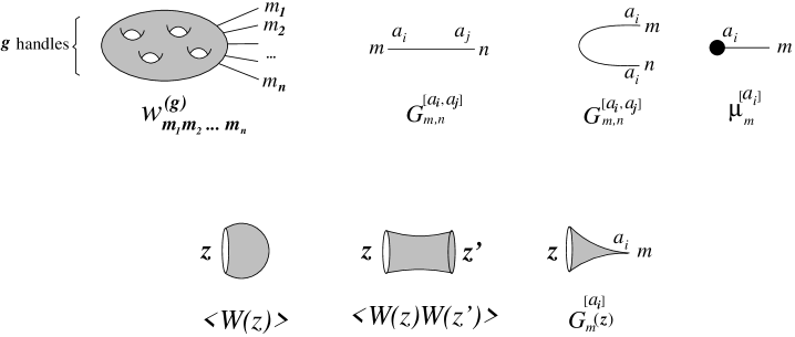
Figure 2: The Feynman rules for genus expansion of the hermitian matrix model. The vertices $W^{(g)}_{m_{1},\dots,m_{n}}$ are universal, the propagators $G^{[a_{i},a_{j}]}_{m,n}$ depend only on the moduli of the spectral curve, and the tadpoles $\mu_{m}^{[a_{j}]}$ are determined by the expansion of the classical solution at the branch points. The vertices are connected to each other by propagators and the tadpoles are connected directly to the vertices. The Feynman graphs for the correlation functions of the resolvent contain three more elements: the disk, the cylinder and the external legs depicted in the second line.

The correlators of the resolvent of the random matrix are obtained from the correlations of the current $J$ by the identification (2.12). To evaluate the correlation functions of the current we use its representation as differential operator

$$\hat{J}(z)=J_{c}(z)+\sum_{j=1}^{2p}\sum_{n\geq 0}G^{[a_{j}]}_{n}(z)\ \partial^{[a_{j}]}_{n}.$$ (4.31)

We therefore extend the set of Feynman rules by adding the external lines which represent the functions

$$G^{[a_{j}]}_{n}(z)=2\int{dz^{\prime}\over 2\pi i}\ {\langle J(z)J(z^{\prime})\rangle\over(z^{\prime}-a_{j})^{n+1/2}}\,.$$ (4.32)

The Feynman rues for evaluating the $1/N$ expansion are given in Fig. 2. The genus $g$ contribution for any observable is equal to the sum of all genus $g$ Feynman diagrams. The genus of a Feynman diagram is equal to $2-2h-n$, where $h$ is the number of handles, including the handles made of propagators, and $n$ is the number of the external lines.

5 Example: the single cut solution

In this section we consider in details the case of one cut $(p=1)$, where the Riemann surface of the classical solution is a sphere. The explicit expression for the classical current is

$$J_{c}(z)={\textstyle{1\over 2}}\oint_{A_{1}}{dz\over 2\pi i}{y(z)\over y(z^{\prime})}\ {V^{\prime}(z^{\prime})-V^{\prime}(z)\over z-z^{\prime}},\qquad y(z)=\sqrt{(z-a_{1})(z-a_{2})}.$$ (5.1)

Expanding at $z=\infty$ and using the asymptotics $J_{c}(z)\sim-{1\over 2}V^{\prime}(z)+{N/z}+...$, one finds the conditions

$$\oint_{A_{1}}{dz\over 2\pi i}{z^{k}V^{\prime}(z)\over y(z)}=-2N\delta_{k,1}\quad\quad(k=0,1)\,$$ (5.2)

which determine the positions of the two branch points.

The two-point function of the ${\mathbb{Z}}_{2}$-twisted current $J(z)$ on the Riemann surface of the classical solution is equal to the 4-point function of two currents and two twist operators:

$$\langle J(z)J(z^{\prime})\rangle\equiv\langle 0|J(z)J(z^{\prime})\sigma(a)\sigma(b)|0\rangle={{\sqrt{(z-a_{1})(z^{\prime}-a_{2})\over(z-a_{2})(z^{\prime}-a_{1})}}+{\sqrt{(z^{\prime}-a_{1})(z-a_{2})\over(z^{\prime}-a_{2})(z-a_{1})}}\over 4(z-z^{\prime})^{2}}.$$ (5.3)

The coefficients $G^{[a_{i},a_{k}]}_{km}$ are obtained by expanding $\langle J(z)J(z^{\prime})\rangle$ near the points $a_{1}$ and $a_{2}$. Assuming that $a_{2}>a_{1}$, we write

$$G^{[a_{i},a_{j}]}_{km}=4\oint_{a_{i}}{dz\over 2\pi i}\oint_{a_{j}}{dz_{j}\over 2\pi i}\ (z-a_{i})^{-k-{1\over 2}}(z^{\prime}-a_{j})^{-m-{1\over 2}}\ \langle J(z)J(z^{\prime})\rangle.$$ (5.4)

We find that $G^{[a_{1},a_{1}]}_{km}$ are of the form

$$G^{[a_{i},a_{k}]}_{k,m}={1\over d^{k+m+1}}\ g^{[a_{i},a_{k}]}_{km},\qquad d=|a_{1}-a_{2}|,$$ (5.5)

where $g^{[a_{i},a_{j}]}_{km}$ are rational numbers with the symmetry $g^{[a_{1},a_{1}]}_{km}=g^{[a_{2},a_{2}]}_{km}$ and $g^{[a_{1},a_{2}]}_{km}=g^{[a_{2},a_{1}]}_{km}$. The first several coefficients $g^{[a_{i},a_{j}]}_{km}$ are

$$\{g^{(a_{1},a_{1})}_{km}\}_{{}_{k,m\geq 0}}=\{g^{(a_{2},a_{2})}_{km}\}_{{}_{k,m\geq 0}} = {\begin{pmatrix}-{1/2}&{3/8}&-{5/16}&...\\ {3/8}&-{3/8}&{45/128}&...\\ -{5/16}&{45/128}&-{45/128}&...\\ .\ .\ .&.\ .\ .&.\ .\ .&\\ \end{pmatrix}}$$

$$\{g^{(a_{1},a_{2})}_{km}\}_{{}_{k,m\geq 0}}=\{g^{(a_{2},a_{1})}_{km}\}_{{}_{k,m\geq 0}} = {\begin{pmatrix}-{1}&{3/2}&-{15/8}&...\\ {3/2}&-21/4&165/16&...\\ -15/8&165/16&-1745/64&...\\ .\ .\ .&.\ .\ .&.\ .\ .&\end{pmatrix}}.$$ (5.6)

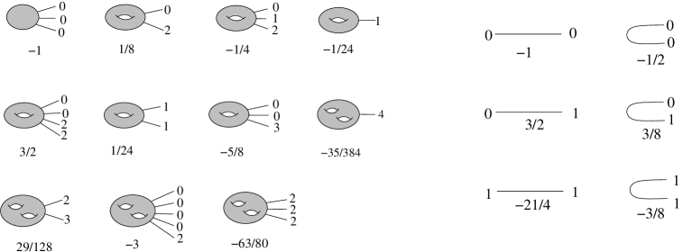
Figure 3: The vertices $w^{(g)}_{m_{1},\dots,m_{n}}$ and the propagators $g^{[a,a^{\prime}]}_{mn}$ and $g^{[a,a]}_{mn}=g^{[a^{\prime},a^{\prime}]}_{mn}$ contributing to the genus two free energy in the case of a single cut.

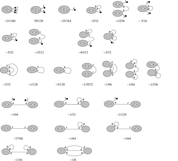
Figure 4: The Feynman graphs contributing to the genus two free energy in the case of a single cut.

As an illustration of the Feynman diagram technique we will evaluate the free energy up to genus two. We denote the two branch points by $a^{\prime}=a_{1}$, $a=a_{2}$, and the moments of the classical solution associated with them by $\mu_{n}=\mu_{n}^{(a)},\mu^{\prime}_{n}=\mu_{n}^{(a^{\prime})}$.

The genus-one term is

$${\cal F}^{(1)} = -{1\over 24}\ln\mu_{1}-{1\over 24}\ln\mu^{\prime}_{1}-{1\over 8}\ln d\qquad(d=a-a^{\prime}).$$ (5.7)

The first two terms come from the dressing of the twist operators and the last term is the logarithm of the correlation function $\langle 0|\sigma(a^{\prime})\sigma(a)|0\rangle$.

The term ${\cal F}^{(2)}$ in the genus expansion of the free energy is a sum of the contributions of all possible genus two Feynman diagrams composed by the vertices and the propagators shown in Fig. 3. The relevant diagrams are depicted in Fig. 4. The result is

$${\cal F}^{(2)} = {1\over\mu_{1}^{2}}\left(-{21\over 160}{\mu_{2}^{3}\over\mu_{1}^{3}}+{29\over 128}{\mu_{2}\mu_{3}\over\mu_{1}^{2}}-{35\over 384}{\mu_{4}\over\mu_{1}}+{5\over 32}{\mu_{3}\over\mu_{1}d}-{49\over 256}{\mu_{2}^{2}\over\mu_{1}^{2}d}-{105\over 512}{\mu_{2}\over d^{2}\mu_{1}}-{175\over 1024}{1\over d^{3}}\right)$$ (5.8)

$$+ \{\mu\leftrightarrow\mu^{\prime}\}\ \ +{1\over\mu_{1}\mu^{\prime}_{1}}\left(-{1\over 64}{\mu_{2}\mu^{\prime}_{2}\over\mu_{1}\mu^{\prime}_{1}d}-{5\over 128}{\mu_{2}\over\mu_{1}d^{2}}-{5\over 128}{\mu^{\prime}_{2}\over\mu^{\prime}_{1}d^{2}}-{69\over 256}{1\over d^{3}}\right)$$

The genus two free energy was first computed by Ambjorn et al in [3]. To compare with the result of [3] we have to express the moments $\mu_{n}$ and $\mu^{\prime}_{n}$ of the classical field in terms of the ACKM moments $M_{n}$ and $J_{n}$, defined as

$$M_{n} = -{2\over N}\oint{dz\over 2\pi i}\ {J_{c}(z)\over(z-a)^{n+1/2}(z-a^{\prime})^{1/2}}\ ={1\over N}\sum_{k=0}^{n-1}{(2k-1)!!\over k!(-2d)^{k}}\mu_{n-k},,$$

$$J_{n} = -{2\over N}\oint{dz\over 2\pi i}\ {J_{c}(z)\over(z-a)^{1/2}(z-a^{\prime})^{n+1/2}}=(-1)^{n-1}{1\over N}\sum_{k=0}^{n-1}{(2k-1)!!\over k!(-2d)^{k}}\mu^{\prime}_{n-k}.$$ (5.9)

Substituting (5) in the answer found in [3] (note that some of the coefficients are corrected in [24])

$$N^{2}{\cal F}^{(2)} = -{181\over 480J_{1}^{2}d^{4}}-{181\over 480M_{1}^{2}d^{4}}+{181J_{2}\over 480J_{1}^{3}d^{3}}-{181M_{2}\over 480M_{1}^{3}d^{3}}+{3J_{2}\over 64J_{1}^{2}M_{1}d^{3}}$$ (5.10)

$$- {3M_{2}\over 64M_{1}^{2}J_{1}d^{3}}-{11J_{2}^{2}\over 40J_{1}^{4}d^{2}}-{11M_{2}^{2}\over 40M_{1}^{4}d^{2}}+{43M_{3}\over 192M_{1}^{3}d^{2}}$$ (5.11)

$$+ {43J_{3}\over 192J_{1}^{3}d^{2}}+{J_{2}M_{2}\over 64J_{1}^{2}M_{1}^{2}d^{2}}-{5\over 16J_{1}M_{1}d^{4}}+{21J_{2}^{3}\over 160J_{1}^{5}d}-{29J_{2}J_{3}\over 128J_{1}^{4}d}+{35J_{4}\over 384J_{1}^{3}d}$$ (5.12)

$$- {21M_{2}^{3}\over 160M_{1}^{5}d}+{29M_{2}M_{3}\over 128M_{1}^{4}d}-{35M_{4}\over 384M_{1}^{3}d}$$ (5.13)

one reproduces the expression (5.8).

6 Discussion

The CFT formalism was developed before for the continuum limit of a class of matrix models which reduce to Coulomb gas integrals similar to (1.1), such as the SOS and ADE matrix models [25]. The classical solutions considered in [25] correspond to non-hyperelliptic Riemann surfaces with one higher (or even infinite) order branch point at infinity and one simple branch point on the first sheet. The CFT formulation of these models provides a rigorous derivation of the Feynman rules for the genus expansion obtained previously in [26, 27].

In this paper we developed the CFT formalism for any classical solution of the hermitian one-matrix model. We do not see conceptual difficulties to generalize it to any classical solution of the above mentioned models, including the $O(n)$ model.

The Feynman rules that follow from the CFT representation look similar to the diagram technique developed in a larger class of matrix models by Eynard and collaborators [4, 28, 29, 30, 31]. If there exists an exact correspondence between the two formalisms, then the CFT formalism can be possibly extended also for matrix models which do not reduce to Coulomb gas integrals. It is likely that the recipe for transforming the Eynard formalism into an effective field theory proposed by Flume et al. [32] is the way to obtain this correspondence.

Acknowledgments

The author thanks A. Alexandrov, B. Eynard and N. Orantin for useful discussions.

References

- [1] I. Kostov, “Conformal field theory techniques in random matrix models,” arXiv:hep-th/9907060.
- [2] E. Brezin, C. Itzykson, G. Parisi, and J. B. Zuber, “Planar Diagrams,” Commun. Math. Phys. 59 (1978) 35.
- [3] J. Ambjorn, L. Chekhov, C. F. Kristjansen, and Y. Makeenko, “Matrix model calculations beyond the spherical limit,” Nucl. Phys. B404 (1993) 127–172, arXiv:hep-th/9302014.
- [4] B. Eynard, “Topological expansion for the 1-hermitian matrix model correlation functions,” JHEP 11 (2004) 031, arXiv:hep-th/0407261.
- [5] G. Moore, “Geometry of the string equations,” Commun. Math. Phys. 2 (1990) no. 2, 261–304.
- [6] A.Alexandrov, A.Mironov, and A.Morozov, “BGWM as Second Constituent of Complex Matrix Model,” arXiv:hep-th/0906.3305.
- [7] A. S. Alexandrov, A. Mironov, A. Morozov, and P. Putrov, “Partition Functions of Matrix Models as the First Special Functions of String Theory. II. Kontsevich Model,” arXiv:0811.2825 [hep-th].
- [8] A.Alexandrov, A.Mironov, and A.Morozov, “Instantons and Merons in Matrix Models,” Physica D 235 (2007) 126–167, hep-th/0608228.
- [9] A. Marshakov, A. Mironov, and A. Morozov, “Generalized matrix models as conformal field theories: Discrete case,” Phys. Lett. B265 (1991) 99–107.
- [10] S. Kharchev, A. Marshakov, A. Mironov, A. Morozov, and S. Pakuliak, “Conformal matrix models as an alternative to conventional multimatrix models,” Nucl. Phys. B404 (1993) 717–750, arXiv:hep-th/9208044.
- [11] A. Morozov, “Matrix models as integrable systems,” arXiv:hep-th/9502091.
- [12] G. Bonnet, F. David, and B. Eynard, “Breakdown of universality in multi-cut matrix models,” J. Phys. A33 (2000) 6739–6768, arXiv:cond-mat/0003324.
- [13] A. B. Zamolodchikov, “Conformal scalar field on the hyperelliptic curve and the critical Ashkin-Teller multipoint correlation functions,” Nucl. Phys. B285 (1987) 481–503.
- [14] L. J. Dixon, D. Friedan, E. J. Martinec, and S. H. Shenker, “he Conformal Field Theory of Orbifolds,” Nucl. Phys. 1987 (B282) 13–73.
- [15] V. G. Knizhnik, “Analytic fields on Riemann surfaces,” Phys. Lett. B180 (1986) 247.
- [16] V. G. Knizhnik, “Analytic Fields on Riemann Surfaces. 2,” Commun. Math. Phys. 112 (1987) 567–590.
- [17] V. G. Knizhnik, “Multiloop amplitudes in the theory of quantum strings and complex geometry,” Sov. Phys. Usp. 32 (1989) 945–971.
- [18] R. Dijkgraaf, A. Sinkovics, and M. Temurhan, “Matrix Models and Gravitational Corrections,” Adv.Theor.Math.Phys. 7 (2004) 1155–1176, hep-th/0211241.
- [19] T. Miwa, “CLIFFORD OPERATORS AND RIEMANN’S MONODROMY PROBLEM,” Publ. Res. Inst. Math. Sci. Kyoto 17 (1981) 665.
- [20] M. R. Gaberdiel, A. O. Klemm, and I. Runkel, “Matrix model eigenvalue integrals and twist fields in the su(2)-WZW model,” JHEP 0510 (2005) 107, hep-th/0509040.
- [21] C. Itzykson and J.-B. Zuber, “Combinatorics of the Modular Group II: the Kontsevich integrals,” Int.J.Mod.Phys. A7 (1992) 5661–5705, hep-th/9201001.
- [22] M. Kontsevich, “Intersection theory on the moduli space of curves and the matrix Airy function,” Commun. Math. Phys. 147 (1992) 1–23.
- [23] M. Bergere and B. Eynard, “Universal scaling limits of matrix models, and (p,q) Liouville gravity,” arXiv:0909.0854 [math-ph].
- [24] J. Ambjorn, L. Chekhov, C. F. Kristjansen, and Y. Makeenko, “erratum,” Nucl. Phys. B 449 (1995) 681.
- [25] I. Kostov and V. Petkova, “Non-Rational 2D Quantum Gravity II. Target Space CFT,” Nucl.Phys.B 769 (2007) 175–216, hep-th/0609020.
- [26] S. Higuchi and I. Kostov, “Feynman rules for string field theories with discrete target space,” Phys. Lett. B357 (1995) 62–70, arXiv:hep-th/9506022.
- [27] I. Kostov, “Solvable statistical models on a random lattice,” Nucl. Phys. Proc. Suppl. 45A (1996) 13–28, arXiv:hep-th/9509124.
- [28] L. Chekhov, B. Eynard, and N. Orantin, “Free energy topological expansion for the 2-matrix model,” JHEP 12 (2006) 053, arXiv:math-ph/0603003.
- [29] L. Chekhov and B. Eynard, “Matrix eigenvalue model: Feynman graph technique for all genera,” JHEP 12 (2006) 026, arXiv:math-ph/0604014.
- [30] B. Eynard and A. P. Ferrer, “Topological expansion of the chain of matrices,” http://arxiv.org/abs/0805.1368.
- [31] B. Eynard and N. Orantin, “Algebraic methods in random matrices and enumerative geometry,” arXiv:0811.3531 [math-ph].
- [32] R. Flume, J. Grossehelweg, and A. Klitz, “A Lagrangean formalism for Hermitean matrix models,” Nucl.Phys.B 812 (2009) 322–342, http://arxiv.org/abs/0805.3078.