Oscillation dynamics of active-unsterile neutrino mixing
in a $2+\tilde{1}$ mixing scheme

Abstract

We consider the possibility that sterile neutrinos exist and admit a description as unparticles; we call these unsterile neutrinos. We then examine the nature of neutrino oscillations in a model where an unsterile can mix with two active flavors with a very simple mass matrix of the see-saw type. Despite these simplifications, we find a number of remarkable features, all of which will occur generically when more realistic cases are considered. These include momentum dependent mixing angles, “invisible” decay widths for the unsterile-like mode, as well as the inheritance of a non-vanishing spectral density for the massive active-like modes. We also obtain the disappearance and appearance probabilities for the active-like neutrinos and find remarkable interference effects between the active and unsterile neutrinos as a consequence of threshold effects, yielding new oscillatory contributions with different oscillation lengths. These effects are only measurable on short baseline experiments because there both probabilities are suppressed as compared to mixing with a canonical sterile neutrino, thereby providing a diagnostics tool to discriminate unsterile from canonical sterile neutrinos. We conclude with a discussion of whether these new phenomena could aid in the reconciliation of the LSND and MiniBooNE results.

I Introduction

Neutrino masses and oscillations are now an established phenomenon and indisputable evidence of physics beyond the standard model. Although the origin and scale of these masses remains a challenging question, the see-saw mechanism provides a compelling framework on how to explain the small active neutrino masses seesaw .

One particular extension of the Standard Model consists of adding the so called sterile neutrinos, which are massive $SU(2)$ singlets. Scenarios involving sterile neutrinos with mass in the $\mathrm{GeV}$ range have been proposed as explanations of two seemingly unrelated and unexpected phenomena: an excess of air shower events at the SHALON gamma ray telescope shalon , and the prominent peak of electron-neutrino events above background for $300\,\mathrm{MeV}\leq E_{\nu}\leq 475\,\mathrm{MeV}$ at the MiniBooNE miniboone . Examples of such scenarios include a 3+2 oscillation scheme involving three active neutrinos and two sterile neutrinos proposed in Ref. maltoni , and an alternative explanation invoking the radiative decay of the heavy sterile neutrino with a small magnetic moment proposed in Ref. gninenko .

Recently, Georgi georgi suggested another extension of the Standard Model, which includes a “hidden” conformal invariant sector with a non-trivial infrared fixed point. This conformal sector can be realized by a renormalization flow toward the infrared through dimensional transmutation banks ; fox . Below the dimensional transmutation scale, there emerges an effective interpolating field, the unparticle field, that features an anomalous scaling dimension. Various studies recognized important phenomenological georgi ; cheung ; spin12 ; ira ; Liao:2007ic ; zwicky1 ; flavor ; parity ; chiumanho , astrophysical raffelt ; deshpande ; freitas and cosmological macdonald ; davo ; lewis ; kame ; he ; kiku ; xuelei ; rich ; unparticleus consequences of unparticles. The consequences of the existence of scalar unparticles in the neutrino sector have also been studied. A scenario where the heaviest mass eigenstates corresponding to the mixed $\nu_{\mu}-\nu_{e}$ decaying into the lightest eigenstate and a scalar unparticle has been suggested as an explanation of the MiniBooNE anomaly liliu ; Zhou:2007zq . Furthermore, unparticle contributions to the neutrino-nucleon cross section and its influence on the neutrino flux expected in a neutrino telescope such as IceCube have been reported in Ref. telescopes .

The question arises whether interesting physics might be found by combining these two ideas. Thus, suppose that sterile neutrinos do exist, and furthermore, they admit a description in terms of unparticles. What consequences arise for neutrino physics, and in particular, neutrino oscillations?

In Ref. Boyanovsky:2009ke , we considered the sterile neutrino to be an unparticle, namely an unsterile neutrino, and studied the mixing of an active and an unsterile neutrino, which revealed unexpected momentum dependence of the mixing angles. Here, we extend that model by including a second active neutrino, and study the consequences in neutrino oscillations. To be precise, we consider a $2+\tilde{1}$ scheme in which two massless active neutrinos mix with an unsterile neutrino via a simple mass matrix of the see-saw type that mixes the active neutrinos only with the unsterile one. Despite the simplicity of the mass matrix, a number of results arise that will persist in more complex models.

We find that the unsterile-active mixing angle depends on the four-momentum and that the propagating modes consist of a massless active-like mode, a massive active-like mode and an unsterile-like mode. The structure of propagators of the massive active-like mode and the unsterile-like mode are similar to the ones found in Boyanovsky:2009ke .

To study the dynamics of active-active oscillation, we generalize the conventional quantum mechanical description of neutrino oscillations in terms of the propagators of mass eigenstates and calculate the appearance and disappearance probabilities. The oscillation dynamics reveals remarkable interference phenomena associated with the threshold of the inherited spectral density for the massive active-like and the complex unsterile-like pole. The momentum dependent mixing angles along with these novel interference contributions yield new oscillatory contributions to the appearance and disappearance probabilities of the active neutrinos with a different oscillation length. These new contributions will be manifest as quantum beats as a function of energy and baseline in oscillation experiments. The non-oscillatory contributions to these probabilities are suppressed with respect to the case of a canonical sterile neutrino, which has no anomalous dimension.

Recently, in Ref. Schwetz:2007cd , it has been proposed that energy dependent mixing and or oscillation parameters may reconcile the LSND lsnd and MiniBooNE miniboone data. This suggestion hinges on the possibility of “exotic” sterile neutrinos whose mixing with the active ones features novel energy dependent mixing angles and/or oscillation parameters. The energy dependence may reconcile the results of both experiments which are performed in different energy regimes ($\sim 40\,\mathrm{MeV}$ for LSND, vs. $\sim\,\mathrm{GeV}$ for MiniBooNE). Given the energy dependence we find in our analysis, we were motivated to see whether our model could be of use in understanding how the LSND and MiniBooNE data mesh together. For our model, we find that we cannot reconcile the data, but that might be attributable to not having enough structure in the mass matrix.

II $2+\tilde{1}$ Scheme

The Lagrangian density for the unsterile in momentum space is Boyanovsky:2009ke

$$\mathcal{L}=\overline{\psi}_{U}(-p)\,\big{(}\not\!{p}-M\big{)}F(p)\,\psi_{U}(p),$$ (1)

where

$$F(p)=\Big{[}\frac{-p^{2}+M^{2}-i0^{+}}{\Lambda^{2}}\Big{]}^{-\eta}~{}~{},~{}~{}0\leq\eta<1\,.$$ (2)

$\Lambda$ is the scale below which the low energy dynamics is dominated by the infrared fixed point of the conformal sector. Below this scale the unparticle is described by an interpolating field whose two point correlation function scales with an anomalous dimension. Consistency of the unparticle interpretation requires that $M<\Lambda$, where $M$ is the infrared cut-off or unparticle threshold. This Lagrangian density can be understood using a renormalization group resummation argument discussed in Ref. Boyanovsky:2009ke and references therein.

We consider a see-saw type mixing with two active Dirac neutrinos, such that the full momentum space Lagrangian density is given by

$$\mathcal{L}=\left(\begin{array}[]{ccc}\overline{\nu}_{a_{1}}(-p)&\overline{\nu}_{a_{2}}(-p)&\overline{\psi}_{U}(-p)\end{array}\right)\,\left(\begin{array}[]{ccc}\not\!{p}&0&-m_{1}\\ 0&\not\!{p}&-m_{2}\\ -m_{1}&-m_{2}&(\not\!{p}-M)F(p)\end{array}\right)\,\left(\begin{array}[]{c}\nu_{a_{1}}(p)\\ \nu_{a_{2}}(p)\\ \psi_{U}(p)\end{array}\right),$$ (3)

with $\nu_{a_{1,2}}$ are the active neutrinos and we assume $m_{1,2}\ll M<\Lambda$ leading to a see-saw hierarchy of masses. Following Boyanovsky:2009ke , let us introduce a rescaled unsterile field

$$\nu_{U}=\sqrt{F(p)}~{}~{}\psi_{U},$$ (4)

such that the Lagrangian density is now given by

$$\mathcal{L}=\left(\begin{array}[]{ccc}\overline{\nu}_{a_{1}}&\overline{\nu}_{a_{2}}&\overline{\nu}_{U}\end{array}\right)\,\left(\not\!{p}\,\mathds{I}-\mathds{M}\right)\,\left(\begin{array}[]{c}\nu_{a_{1}}\\ \nu_{a_{2}}\\ \nu_{U}\end{array}\right),$$ (5)

where $\mathds{I}$ is the identity in the “flavor” space, and the “mass” matrix is

$$\mathds{M}=\left(\begin{array}[]{ccc}0&0&\frac{m_{1}}{\sqrt{F}}\\ 0&0&\frac{m_{2}}{\sqrt{F}}\\ \frac{m_{1}}{\sqrt{F}}&\frac{m_{2}}{\sqrt{F}}&M\end{array}\right).$$ (6)

We note that $\mathds{M}$ has a zero eigenvalue, which aids considerably in the diagonalization. We reiterate that this mass matrix describes a simplified model, chosen only so as to exhibit the mixing that we want to describe (active-unsterile) while suppressing effects we consider extraneous to the discussion.

This mass matrix can be diagonalized exactly and the fields corresponding to the propagating or “mass” eigenstates are given by

$$\nu_{1} = \frac{-m_{2}\,\nu_{a_{1}}+m_{1}\,\nu_{a_{2}}}{m}\,,$$ (7)

$$\nu_{2} = \frac{2m_{1}\,\nu_{a_{1}}+2m_{2}\,\nu_{a_{2}}-\left(\sqrt{M^{2}F+4m^{2}}-M\sqrt{F}\right)\,\nu_{U}}{\left[2M^{2}F+8m^{2}-2M\sqrt{M^{2}F^{2}+4m^{2}F}\right]^{1/2}}\,,$$ (8)

$$\nu_{3} = \frac{2m_{1}\,\nu_{a_{1}}+2m_{2}\,\nu_{a_{2}}+\left(M\sqrt{F}+\sqrt{M^{2}F+4m^{2}}\right)\,\nu_{U}}{\left[2M^{2}F+8m^{2}+2M\sqrt{M^{2}F^{2}+4m^{2}F}\right]^{1/2}},$$ (9)

with their propagators given by

$$G_{1} = \frac{\not\!{p}}{p^{2}}\,,$$ (10)

$$G_{2} = \frac{\not\!{p}+M_{2}(p)}{p^{2}-M_{2}^{2}(p)}\,;\qquad M_{2}=\frac{M\sqrt{F}-\sqrt{M^{2}F+4m^{2}}}{2\sqrt{F}}\,,$$ (11)

$$G_{3} = \frac{\not\!{p}+M_{3}(p)}{p^{2}-M_{3}^{2}(p)}\,;\qquad M_{3}=\frac{M\sqrt{F}+\sqrt{M^{2}F+4m^{2}}}{2\sqrt{F}}\,,$$ (12)

respectively, where

$$m=\sqrt{m_{1}^{2}+m_{2}^{2}}\,.$$ (13)

The propagators of the massive active-like mode and unsterile-like mode follow closely the propagators of the active-like mode and unsterile-like mode of Ref. Boyanovsky:2009ke .

As in Ref. Boyanovsky:2009ke , we assume that $m_{1,2}\ll M$ and self-consistently

$$\frac{m^{2}}{M^{2}F(p_{2,3})}\ll 1\,.$$ (14)

In this approximation, it is convenient to introduce

$$\epsilon_{1,2}(p)=\frac{m_{1,2}}{M\,\sqrt{F(p)}}~{}~{};~{}~{}\epsilon(p)=\sqrt{\epsilon^{2}_{1}(p)+\epsilon^{2}_{2}(p)}\,,$$ (15)

and the mixing angles

$$\cos\theta=\frac{\epsilon_{1}}{\epsilon}=\frac{m_{1}}{m}~{}~{};~{}~{}\sin\theta=\frac{\epsilon_{2}}{\epsilon}=\frac{m_{2}}{m}~{}~{};$$

$$\cos\Phi=\frac{1}{\sqrt{1+\epsilon^{2}(p)}}~{}~{};~{}~{}\sin\Phi=\frac{\epsilon(p)}{\sqrt{1+\epsilon^{2}(p)}}\,.$$ (16)

We note that whereas the angle $\theta$ does not depend on momentum, the angle $\Phi$ does depend on momentum through $F(p)$.

To leading order in $\epsilon$’s we find

$$M_{2}(p)=-M\epsilon^{2}(p)~{}~{};~{}~{}M_{3}(p)=M\big{[}1+\epsilon^{2}(p)\big{]}\,,$$ (17)

and the fields associated with the propagating eigenstates given by eqs. (7) - (9) can be written as

$$\nu_{1} = -\sin\theta\,\nu_{a_{1}}+\cos\theta\,\nu_{a_{2}}\,,$$ (18)

$$\nu_{2} = \cos\Phi\,\cos\theta\,\nu_{a_{1}}+\cos\Phi\,\sin\theta\,\nu_{a_{2}}-\sin\Phi\,\nu_{U}\,,$$ (19)

$$\nu_{3} = \sin\Phi\,\cos\theta\,\nu_{a_{1}}+\sin\Phi\,\sin\theta\,\nu_{a_{2}}+\cos\Phi\,\nu_{U}\,.$$ (20)

The properties of the propagators can be found by following the calculation in Ref. Boyanovsky:2009ke and in the following, we will summarize the results. For details, see Boyanovsky:2009ke .

II.1 Poles and Spectral Density for the Massive Active-like Mode

Near the pole, the propagator behaves as

$$\frac{1}{p^{2}-M^{2}_{2}(p)}\approx\frac{Z_{2}}{p^{2}-{\cal M}^{2}_{2}}\,,$$ (21)

where

$$Z^{-1}_{2}\approx 1+2\eta~{}\frac{{\cal M}^{2}_{2}}{M^{2}}\,,$$ (22)

and

$${\cal M}^{2}_{2}=\left(\frac{M\Delta}{2}\right)^{2}\,,$$ (23)

with

$$\Delta=2~{}\frac{m^{2}}{M^{2}}\Bigg{[}\frac{M^{2}}{\Lambda^{2}}\Bigg{]}^{\eta}\,.$$ (24)

This is an isolated pole below the unparticle threshold at $p^{2}=M^{2}$. This pole lies on the real $p^{2}$ axis and describes a massive stable active-like propagating mode.

The massive active-like propagator also features an inherited spectral density

$$\rho_{2}(x)=\frac{\Theta(x)}{\pi}~{}\frac{\frac{\Delta^{2}}{4}\,x^{2\eta}\sin(2\pi\eta)}{\Big{[}x+1-\frac{\Delta^{2}}{4}\,x^{2\eta}\cos(2\pi\eta)\Big{]}^{2}+\Big{[}\frac{\Delta^{2}}{4}\,x^{2\eta}\sin(2\pi\eta)\Big{]}^{2}}\,.$$ (25)

where

$$x=\frac{p^{2}-M^{2}}{M^{2}}\,.$$ (26)

The non-vanishing spectral density above the unparticle threshold at $p^{2}=M^{2}$ will lead to interesting new phenomena in the disappearance and appearance probabilities discussed below.

II.2 Complex Poles and Spectral Density for the Unsterile-like Mode

The solution describes a pole in the complex plane (a resonance) and it exists only for

$$\mathrm{Re}(x)>0~{},~{}0\leq\eta<1/3.$$

Near this pole we find

$$\frac{1}{p^{2}-M^{2}_{3}(p)}\approx\frac{Z_{3}}{p^{2}-{\cal M}^{2}_{3}+i{\cal M}_{3}\Gamma}\,,$$ (27)

with

$$Z_{3}=\frac{1}{1-\eta}\,,$$ (28)

$${\cal M}^{2}_{3}=M^{2}\Big{[}1+\Delta^{\frac{1}{1-\eta}}\,\cos\Big{(}\frac{\pi\eta}{1-\eta}\Big{)}\Big{]}\;,$$ (29)

and

$$\Gamma=\frac{M^{2}}{{\cal M}_{3}}\Delta^{\frac{1}{1-\eta}}\,\sin\Big{(}\frac{\pi\eta}{1-\eta}\Big{)}\;.$$ (30)

The imaginary part is a consequence of the fact that the real part of the pole is above the unparticle continuum and it describes the decay of the unsterile like mode into the massive active-like mode and particles in the “hidden” conformal sector. This can be understood using a renormalization group resummation argument presented in Ref. Boyanovsky:2009ke . The spectral density is obtained from the discontinuity across the real axis in the complex $p^{2}$ plane

$$\rho_{3}(x)=\frac{\Theta(x)}{\pi}~{}\frac{\Delta\,x^{\eta}\sin(\pi\eta)}{\Big{[}x-{\Delta}\,x^{\eta}\cos(\pi\eta)\Big{]}^{2}+\Big{[}{\Delta}\,x^{\eta}\sin(\pi\eta)\Big{]}^{2}}\,.$$ (31)

For consistency of the see-saw mechanism, to give small masses to the active-like neutrinos it is required that

$$\Delta=2~{}\frac{m^{2}}{M^{2}}\Bigg{[}\frac{M^{2}}{\Lambda^{2}}\Bigg{]}^{\eta}\ll 1\,,$$ (32)

thus ensuring that $\mathcal{M}_{2}=\frac{1}{2}M\Delta\ll M$.

III Towards Understanding Active-Active Oscillation Dynamics.

The familiar quantum mechanical description of neutrino oscillation invokes single particle quantum mechanical states. The essential ingredients are the expectation values $\langle\nu_{i}|\,e^{-iHt}\,|\nu_{i}\rangle$. In quantum field theory, the (fermionic) fields are expanded in terms of creation and annihilation operators of quanta associated with a Fock basis, which is determined by the spinor basis functions. For the mass eigenstates these are the solutions of the (free) Dirac equation, whereas for flavor states such choice is ambiguous boyahodense . To focus the discussion on a simple case to be generalized later, consider a flavor doublet of Dirac neutrinos with an off-diagonal mass term, with Lagrangian density

$$\mathcal{L}=\overline{\Psi}\Big{[}\not\!{p}-\mathds{M}\Big{]}\Psi\,,$$ (33)

where

$$\Psi=\left(\begin{array}[]{c}\psi_{e}\\ \psi_{\mu}\\ \end{array}\right)~{}~{};~{}~{}\mathds{M}=\left(\begin{array}[]{cc}m_{ee}&m_{e\mu}\\ m_{e\mu}&m_{\mu\mu}\\ \end{array}\right).$$ (34)

Diagonalizing the mass matrix via a unitary transformation leads to the fields $\psi_{1,2}$ associated with the mass eigenstates $m_{1,2}$, related to the flavor fields $\psi_{e,\mu}$ as

$$\psi_{e} = \cos\theta\,\psi_{1}+\sin\theta\,\psi_{2}\,,$$ (35)

$$\psi_{\mu} = \cos\theta\,\psi_{2}-\sin\theta\,\psi_{1}\,.$$ (36)

The neutrino fields $\psi_{1,2}$ are quantized as usual

$$\psi_{i}(\vec{x},0) = \ \frac{1}{\sqrt{V}}\sum_{\vec{k},h=\pm 1}e^{i\vec{k}\cdot\vec{x}}\,\psi_{i}(\vec{k},0)\,,$$

$$\psi_{i}(\vec{k},0) = \Big{[}b_{i}(\vec{k},h)U_{i}(\vec{k},h)+d^{\dagger}_{i}(\vec{k},h)V_{i}(-\vec{k},h)\Big{]}~{}~{};~{}~{}i=1,2$$ (37)

where the annihilation operators $b_{i},d_{i}$ and creation operators $b^{\dagger}_{i},d^{\dagger}_{i}$ obey the usual anticommutation relations and the spinors $U,V$ are solutions of the Dirac equations

$$\big{[}\vec{\alpha}\cdot\vec{k}+\beta m_{i}]U_{i}(\vec{k},h) = E_{i}(k)U_{i}(\vec{k},h)\,,$$ (38)

$$\big{[}\vec{\alpha}\cdot\vec{k}+\beta m_{i}]V_{i}(-\vec{k},h) = -E_{i}(k)V_{i}(-\vec{k},h)\,,$$ (39)

with $E_{i}(k)=\sqrt{k^{2}+m^{2}_{i}}$, and are eigenstates of the helicity operator with eigenvalues $h=\pm 1$. Obviously there is no unambiguous quantization of the flavor spinor fields because there is no unambiguous choice of basis spinors $U,V$ for these boyahodense . One could chose spinor solutions of the massless Dirac equation or with the masses in the diagonal entries in the mass matrix $\mathds{M}$. Any of these choices correspond to spinor solutions which are not orthogonal to any of the solutions of the mass eigenstates (either positive or negative energy) boyahodense .

The positive energy single particle quantum mass eigenstates of helicity $h$ are

$$|\nu_{i}(\vec{k},h)\rangle=b^{\dagger}_{i}(\vec{k},h)\,|0\rangle=\psi^{\dagger}_{i}(\vec{k},0)\,|0\rangle\,U_{i}(\vec{k},h)\,,$$ (40)

$$\langle\nu_{i}(\vec{k},h)|=\langle 0|\,b_{i}(\vec{k},h)=U^{\dagger}_{i}(\vec{k},h)\langle 0|\,\psi_{i}(\vec{k},0)\,.$$ (41)

We define the single particle flavor states as

$$|\nu_{e}\rangle = \cos\theta\,|\nu_{1}\rangle+\sin\theta\,|\nu_{2}\rangle\,,$$ (42)

$$|\nu_{\mu}\rangle = \cos\theta\,|\nu_{2}\rangle-\sin\theta\,|\nu_{1}\rangle\,,$$ (43)

where the quantum numbers $\vec{k},h$ are common to all the states. Since the Hamiltonian is diagonal in the mass basis, the transition amplitudes $\langle\nu_{\alpha}|\,e^{-iHt}\,|\nu_{\beta}\rangle$ ($\alpha,\beta=e,\mu$) require the overlaps

$$\langle\nu_{i}(\vec{k},h)|\,e^{-iHt}\,|\nu_{i}(\vec{k},h)\rangle=U^{\dagger}_{i}(\vec{k},h)\langle 0|\,\psi_{i}(\vec{k},t)\overline{\psi}_{i}(\vec{k},0)\,|0\rangle\,\gamma^{0}U_{i}(\vec{k},h)\,,$$ (44)

where $\psi_{i}(\vec{k},t)$ are the Heisenberg field operators. In terms of the propagator for $t>0$, the overlaps are given by

$$\langle\nu_{i}(\vec{k},h)|\,e^{-iHt}\,|\nu_{i}(\vec{k},h)\rangle=U^{\dagger}_{i}(\vec{k},h)\,\big{(}iS_{i}(\vec{k},t>0)\big{)}\gamma^{0}U_{i}(\vec{k},h)\,,$$ (45)

thereby establishing a direct relation between the quantum field theory propagators for the mass eigenstates and the single particle transition amplitudes.

It is convenient to work in the chiral representation

$$\gamma^{0}=\left(\begin{array}[]{cc}0&-\mathds{I}\\ -\mathds{I}&0\\ \end{array}\right)~{}~{};~{}~{}\vec{\gamma}=\left(\begin{array}[]{cc}0&\vec{\sigma}\\ -\vec{\sigma}&0\\ \end{array}\right)~{}~{};~{}~{}\gamma^{5}=\left(\begin{array}[]{cc}\mathds{I}&0\\ 0&-\mathds{I}\\ \end{array}\right)\,,$$ (46)

in which we find the positive energy spinors for the mass eigenstates with mass $m_{i}$ to be

$$U_{i}(\vec{k},+1) = \sqrt{\frac{E_{i}(k)+k}{2k}}\left(\begin{array}[]{c}v(\vec{k},1)\\ -\frac{m_{i}}{E_{i}(k)+k}\,v(\vec{k},1)\\ \end{array}\right)\,,$$ (49)

$$U_{i}(\vec{k},-1) = \sqrt{\frac{E_{i}(k)+k}{2k}}\left(\begin{array}[]{c}-\frac{m_{i}}{E_{i}(k)+k}\,v(\vec{k},-1)\\ v(\vec{k},-1)\\ \end{array}\right)\,,$$ (52)

where $E_{i}(k)=\sqrt{k^{2}+m^{2}_{i}}$ and the two component spinors are eigenstates of helicity

$$\vec{\sigma}\cdot\widehat{\vec{k}}\,v(\vec{k},h)=h\,v(\vec{k},h)~{};~{}h=\pm 1\,.$$ (53)

The spinors $U$ are normalized to unity and become right handed ($h=1$) or left handed ($h=-1$) respectively in the ultrarelativistic limit. The propagator in real time is given by

$$S_{i}(\vec{k},t)=\int\frac{dp_{0}}{2\pi}e^{-ip_{0}t}S_{i}(p)\,,$$ (54)

and for free field theory

$$S_{i}(p)=\frac{\not\!{p}+m_{i}}{p^{2}-m^{2}_{i}+i0^{+}}\,.$$ (55)

It is straightforward to confirm that for $t>0$ the result of Eq. (45) is $e^{-iE_{i}(k)t}$.

In generalizing the above discussion to the case of active-unsterile mixing, we face two caveats:

1. the mixing angle $\Phi$ in Eq. (16) depends on the four momentum; this is one of the features that prompted the study of unsterile-active mixing as a potential reconciliation of MiniBoone and LSND data as suggested in Ref. Schwetz:2007cd ,

2. the pole of the unsterile-like eigenstate $\nu_{3}$ is complex with the imaginary part being associated with the decay of the sterile neutrino into an active one and quanta of the hidden conformal sector Boyanovsky:2009ke .

A full quantum field theory study along the lines presented in Refs. boyaho ; wuboya incorporates the full propagators and spectral densities, which are dominated by the poles below the continuum threshold in the case of the active-like modes and the complex pole above threshold for the unsterile like mode. The (four) momentum dependence of the mixing angles is then evaluated at the position of these poles (see Refs. boyaho ; wuboya for a detailed discussion). In these references, the dynamics of neutrino oscillations was studied as an initial value problem for an initial wave packet. However, the real oscillation experiment deals with neutrinos produced at a source and detected via charged leptons in a far detector, so that the neutrino is virtual in this process. In this case, the real time quantum field theoretic analysis of oscillation dynamics is more complex. The interaction vertices are written in terms of the fields that create and annihilate the mass eigenstates and “flavor” neutrinos are an intermediate state, described by a propagator associated with the mass eigenstates. Such study is just beginning to emerge, and progress will be reported elsewhere future . A full quantum field theoretical study of active-unsterile dynamics is beyond the scope of this article, but we can extrapolate from the study in Refs. boyaho ; wuboya and take the mixing angles to be associated with the single (quasi) particle states, therefore evaluated on the mass shell of the mass eigenstates corresponding to the poles in the respective propagators.

In the case of the unsterile mode, the imaginary part of the pole (decay width) is subleading in the small ratio $\Delta$ (see Eq. (30)) and we neglect it in the evaluation of the mixing angle $\Phi$ for the mass eigenstate $\nu_{3}$.

Inverting the relation (18-20) and evaluating the mixing angles on the single particle mass shells we obtain,

$$|\nu_{a1}\rangle = \cos\Phi_{2}\cos\theta|\nu_{2}\rangle+\sin\Phi_{3}\cos\theta|\nu_{3}\rangle-\sin\theta|\nu_{1}\rangle\,,$$ (56)

$$|\nu_{a2}\rangle = \cos\Phi_{2}\sin\theta|\nu_{2}\rangle+\sin\Phi_{3}\sin\theta|\nu_{3}\rangle+\cos\theta|\nu_{1}\rangle\,,$$ (57)

$$|\nu_{U}\rangle = -\sin\Phi_{2}|\nu_{2}\rangle+\cos\Phi_{3}|\nu_{3}\rangle\,,$$ (58)

where to leading order in $\Delta$ we find

$$\sin\Phi_{2}\simeq\Bigg{[}\frac{\Delta}{2[1+\frac{\Delta}{2}]}\Bigg{]}^{\frac{1}{2}}~{}~{};~{}~{}\cos\Phi_{2}\simeq\Bigg{[}\frac{1}{1+\frac{\Delta}{2}}\Bigg{]}^{\frac{1}{2}}\,,$$ (59)

$$\sin\Phi_{3}=\frac{\delta}{\sqrt{1+\delta^{2}}}~{}~{};~{}~{}\cos\Phi_{3}=\frac{1}{\sqrt{1+\delta^{2}}}\,,$$ (60)

and

$$\delta=\sqrt{\frac{\Delta}{2}}\,\Bigg{[}\Delta^{\frac{1}{1-\eta}}\,\cos\Big{(}\frac{\pi\eta}{1-\eta}\Big{)}\Big{]}\Bigg{]}^{\frac{\eta}{2}}\,.$$ (61)

We will focus on negative helicity positive energy states, for which the spinor wave functions are given by Eq. (52).

An immediate caveat of this formulation is that as a consequence of the four-momentum dependence of the mixing angle $\Phi$, the states $\nu_{a1,a2,U}$ introduced above as a straightforward generalization of the familiar quantum mechanical description, are not orthogonal, despite the orthogonality of the mass eigenstates $\nu_{1,2,3}$. This is because $\Phi_{2}\neq\Phi_{3}$. This is an unavoidable consequence of the energy-momentum dependence of the mixing angle and of the effort to establish a correspondence with the familiar single particle quantum mechanical description of an inherently many particle problem. The non-orthogonality of these states is small for $\Delta\ll 1$ as manifest by Eqs. (59,60,61).

While the single particle quantum mechanical analogy has limitations in absence of a full quantum field theory treatment of neutrino mixing and oscillations directly in real time, we adopt the approximate single particle description afforded by (56,57,58) as a proxy description and proceed to explore this formulation as a prelude towards a firmer understanding. A thorough field theoretical description of real time oscillations is postponed for future work.

The fields associated with the mass eigenstates $\psi_{i},i=1,2,3$ are expanded at $t=0$ just as in Eq. (37) but with the spinors $U,V$ solutions of the Dirac equations with masses

$$\mathcal{M}_{1}=0,~{}~{}\mathcal{M}_{2}=\frac{1}{2}M{\Delta},~{}~{}\mathcal{M}_{3}=M\Big{[}1+\Delta^{\frac{1}{1-\eta}}\,\cos\Big{(}\frac{\pi\eta}{1-\eta}\Big{)}\Big{]}^{\frac{1}{2}}\,,$$

respectively Bjorken:1979dk . The annihilation operators $b(\vec{k},h),\,d(\vec{k},h)$ and creation operators $b^{\dagger}(\vec{k},h),\,d^{\dagger}(\vec{k},h)$ are interpolating Heisenberg field operators whose time evolution is determined by the total Hamiltonian such that Bjorken:1979dk

$$\langle 0|\,\psi_{i}(\vec{k},t)\overline{\psi}_{i}(\vec{k},0)\,|0\rangle=S_{i}(\vec{k},t>0)\,.$$ (62)

In order to carry out the integration in $p_{0}$ as in Eq. (54), it is convenient to write the propagators in terms of their spectral representation Bjorken:1979dk

$$S_{i}(p)=\int_{0}^{\infty}dQ^{2}~{}\frac{\not\!{p}\,\rho^{(1)}_{i}(Q^{2})+\mathcal{M}_{i}\,\rho^{(2)}_{i}(Q^{2})}{p^{2}-Q^{2}+i0^{+}}\,,$$ (63)

from which we find

$$S_{i}(\vec{k},t>0)=\int_{0}^{\infty}dQ^{2}~{}\frac{\widetilde{\not\!{p}}\,\rho^{(1)}_{i}(Q^{2})+\mathcal{M}_{i}\,\rho^{(2)}_{i}(Q^{2})}{2E_{i}(Q)}\,e^{-i\mathcal{E}(Q)t}\,,$$ (64)

where

$$\mathcal{E}(Q)=\sqrt{k^{2}+Q^{2}}~{}~{};~{}~{}\widetilde{\not\!{p}}=\gamma_{0}\,\mathcal{E}(Q)-\vec{\gamma}\cdot\vec{k}\,.$$ (65)

To leading order in $\Delta$, we have $\rho_{i}^{(1)}(Q^{2})=\rho_{i}^{(2)}(Q^{2})~{}~{};~{}~{}i=2,3$. For the massive active-like mode

$$\rho^{(1)}_{2}(Q^{2})=Z_{2}\,\delta(Q^{2}-\mathcal{M}^{2}_{2})+\frac{\rho_{2}(x)}{M^{2}}~{}~{};~{}~{}x=\frac{Q^{2}-M^{2}}{M^{2}}\,,$$ (66)

where $Z_{2}$ is given by Eq. (22) and $\rho_{2}(x)$ by Eq. (25). For the unsterile like mode

$$\rho_{3}^{(1)}(Q^{2})=\frac{\rho_{3}(x)}{M^{2}}\,,$$ (67)

where $\rho_{3}(x)$ is given by Eq. (31). Near the complex pole in the continuum, the propagator for the unsterile-like neutrino can be approximated the Breit-Wigner form Eq. (27), which for $\Delta,\eta\ll 1$ describes a narrow resonance near the real axis.

For long times, the integral over the dispersive variable is dominated by the pole and the continuum threshold. The technical details of the evaluation of the threshold contribution are found in the appendix (see Eq. (102)). For negative helicity states, we find

$$\langle\nu_{1}|\,e^{-iHt}\,|\nu_{1}\rangle = e^{-iE_{1}(k)t}\,,$$ (68)

$$\langle\nu_{2}|\,e^{-iHt}\,|\nu_{2}\rangle = Z_{2}\,e^{-iE_{2}(k)t}+\frac{A_{2}}{2\,i^{1+2\eta}}\Bigg{(}\frac{E_{M}}{M^{2}\,t}\Bigg{)}^{1+2\eta}\,e^{-iE_{M}(k)t}\,,$$ (69)

$$\langle\nu_{2}|\,e^{-iHt}\,|\nu_{2}\rangle = Z_{3}\,e^{-iE_{3}(k)t}\,e^{-\frac{\Gamma\,t}{2\gamma}}\,,$$ (70)

where $E_{i}(k)=\sqrt{k^{2}+\mathcal{M}^{2}_{i}}$, $\Gamma$ is given by Eq. (30), $\gamma=E_{3}(k)/\mathcal{M}_{3}$ is the Lorentz time dilation factor and (see appendix, Eq. (103))

$$A_{2}=\frac{\Delta^{2}}{4\pi}\,\sin(2\pi\eta)\,\Gamma(1+2\eta)\,.$$ (71)

The extra factor $1/2$ in (69) as compared to the bosonic case studied in the appendix (see Eq. (102)) is a result of the spinor overlaps in the limit $\Delta\ll 1$.

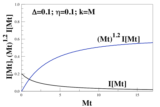
Figure 1: The continuum integral $I[Mt]=|\langle\nu_{2}|\,e^{-iHt}\,|\nu_{2}\rangle|_{cont}/A_{2}$.

The result in Eq. (69) is valid in the long time limit when the threshold contribution dominates the integral over the continuum brown . Fig. (1) displays the integral over the continuum and confirms its asymptotic long time limit.

We are now in position to obtain the active neutrino disappearance and appearance probabilities of active-like neutrinos.

III.1 Disappearance probabilities

The disappearance transition amplitudes are given by

$$\langle\nu_{a1}|\,e^{-iHt}\,|\nu_{a1}\rangle = \sin^{2}\theta\langle\nu_{1}\,|e^{-iHt}\,|\nu_{1}\rangle+\cos^{2}\Phi_{2}\cos^{2}\theta\,\langle\nu_{2}\,|e^{-iHt}\,|\nu_{2}\rangle$$ (72)

$$+\,\sin^{2}\Phi_{3}\cos^{2}\theta\,\langle\nu_{3}\,|e^{-iHt}\,|\nu_{3}\rangle\,,$$

$$\langle\nu_{a2}\,|e^{-iHt}\,|\nu_{a2}\rangle = \cos^{2}\theta\langle\nu_{1}\,|e^{-iHt}\,|\nu_{1}\rangle+\cos^{2}\Phi_{2}\sin^{2}\theta\,\langle\nu_{2}\,|e^{-iHt}\,|\nu_{2}\rangle$$ (73)

$$+\,\sin^{2}\Phi_{3}\sin^{2}\theta\,\langle\nu_{3}\,|e^{-iHt}\,|\nu_{3}\rangle\,,$$

where the transition amplitudes $\langle\nu_{i}\,|e^{-iHt}\,|\nu_{i}\rangle\,;i=1,2,3$ are given by Eqs.(68-70). In obtaining the probabilities there are several interference terms which manifest themselves on different time scales. We will only keep the slow oscillatory terms involving the differences

$$E_{1}(k)-E_{2}(k)\approx\mathcal{M}^{2}_{2}/2k\qquad{\rm and}\qquad E_{M}(k)-E_{3}(k)\approx(\mathcal{M}^{2}_{3}-M^{2})/2E_{M}(k)$$

in the ultrarelativistic limit, and neglect phases that oscillate on much shorter time scales, since these average out. As is customary, we replace time by the baseline $t\rightarrow L$, and define

$$\tilde{A}(L)=\frac{A_{2}}{2}\Bigg{[}\frac{E_{M}(k)}{M^{2}L}\Bigg{]}^{1+2\eta}~{}~{};~{}~{}\xi=\frac{\pi}{2}(1+2\eta)\,.$$ (74)

We then have

$$\mathcal{P}_{a_{1}\rightarrow a_{1}}(L) = Z^{2}_{2}\cos^{4}\Phi_{2}\cos^{4}\theta+\sin^{4}\theta+\frac{Z_{2}}{2}\cos^{2}\Phi_{2}\sin^{2}2\theta\cos\left[\frac{\mathcal{M}^{2}_{2}\,L}{2k}\right]+\,\tilde{A}^{2}(L)\cos^{4}\Phi_{2}\cos^{4}\theta$$ (75)

$$+\,2\,\tilde{A}(L)\,Z_{3}\cos^{2}\Phi_{2}\sin^{2}\Phi_{3}\cos^{4}\theta\,e^{-\frac{\Gamma}{2\gamma}L}\,\cos\left[\frac{(M^{2}-\mathcal{M}^{2}_{3})L}{2E_{M}(k)}+\xi\right]$$

$$+\,Z^{2}_{3}\sin^{4}\Phi_{3}\cos^{4}\theta\,e^{-\frac{\Gamma}{\gamma}L}\,,$$

$$\mathcal{P}_{a_{2}\rightarrow a_{2}}(L) = Z^{2}_{2}\cos^{4}\Phi_{2}\sin^{4}\theta+\cos^{4}\theta+\frac{Z_{2}}{2}\cos^{2}\Phi_{2}\sin^{2}2\theta\cos\left[\frac{\mathcal{M}^{2}_{2}\,L}{2k}\right]+\,\tilde{A}^{2}(L)\cos^{4}\Phi_{2}\sin^{4}\theta$$ (76)

$$+\,2\,\tilde{A}(L)\,Z_{3}\cos^{2}\Phi_{2}\sin^{2}\Phi_{3}\sin^{4}\theta\,e^{-\frac{\Gamma}{2\gamma}L}\,\cos\left[\frac{(M^{2}-\mathcal{M}^{2}_{3})L}{2E_{M}(k)}+\xi\right]$$

$$+\,Z^{2}_{3}\sin^{4}\Phi_{3}\sin^{4}\theta\,e^{-\frac{\Gamma}{\gamma}L}\,.$$

III.2 Appearance probability

From the transition amplitude

$$\langle\nu_{a1}\,|e^{-iHt}\,|\nu_{a2}\rangle=\frac{1}{2}\sin 2\theta\Big{\{}\cos^{2}\Phi_{2}\,\langle\nu_{2}\,|e^{-iHt}\,|\nu_{2}\rangle+\sin^{2}\Phi_{3}\,\langle\nu_{3}\,|e^{-iHt}\,|\nu_{3}\rangle-\langle\nu_{1}\,|e^{-iHt}\,|\nu_{1}\rangle\Big{\}}\,,$$ (77)

by keeping only the slow interference terms and again replacing $t\rightarrow L$, where $L$ is the baseline, we find

$$\mathcal{P}_{a_{1}\rightarrow a_{2}}(L)=\mathcal{P}_{a_{2}\rightarrow a_{1}}(L) = \frac{\sin^{2}2\theta}{4}\Bigg{\{}1+\left[Z^{2}_{2}+\tilde{A}^{2}(L)\right]\cos^{4}\Phi_{2}-2Z_{2}\cos^{2}\Phi_{2}\cos\left[\frac{\mathcal{M}^{2}_{2}\,L}{2k}\right]$$ (78)

$$+\,2\,\tilde{A}(L)\,Z_{3}\cos^{2}\Phi_{2}\sin^{2}\Phi_{3}\,e^{-\frac{\Gamma}{2\gamma}L}\,\cos\Big{[}\frac{(M^{2}-\mathcal{M}^{2}_{3})L}{2E_{M}(k)}+\xi\Big{]}$$

$$+\,Z^{2}_{3}\sin^{4}\Phi_{3}\,e^{-\frac{\Gamma}{\gamma}L}\Bigg{\}}\,,$$

where for $\Delta\ll 1$, it follows that

$$\mathcal{M}^{2}_{3}-M^{2}=M^{2}\Delta^{\frac{1}{1-\eta}}\,\cos\Big{(}\frac{\pi\eta}{1-\eta}\Big{)}\,.$$ (79)

III.3 Consequences of the anomalous dimension

The unsterile neutrino is characterized by the anomalous dimension $\eta$, which is responsible for $\tilde{A},Z_{2},Z_{3},\Gamma\neq 0$ and $\Phi_{3}\neq\Phi_{2}$. Therefore it is important to quantify the potential phenomenological effects of the appearance and disappearance probabilities associated with a non-vanishing (and perhaps large) anomalous dimension. For $\eta=0$, these transition probabilites are the following (we neglect terms that oscillate on the time scale $1/M\ll k/\mathcal{M}^{2}_{2}$ and average out)

$$\mathcal{P}_{a_{1}\rightarrow a_{1}}=\big{(}\cos^{2}\Phi\cos^{2}\theta+\sin^{2}\theta\big{)}^{2}+\sin^{4}\Phi\cos^{4}\theta-\cos^{2}\Phi\sin^{2}(2\theta)\sin^{2}\Big{[}\frac{\mathcal{M}^{2}_{2}L}{4k}\Big{]}\,,$$ (80)

$$\mathcal{P}_{a_{2}\rightarrow a_{2}}=\big{(}\cos^{2}\Phi\sin^{2}\theta+\cos^{2}\theta\big{)}^{2}+\sin^{4}\Phi\sin^{4}\theta-\cos^{2}\Phi\sin^{2}2\theta\sin^{2}\Big{[}\frac{\mathcal{M}^{2}_{2}L}{4k}\Big{]}\,,$$ (81)

$$\mathcal{P}_{a_{1}\rightarrow a_{2}}=\mathcal{P}_{a_{2}\rightarrow a_{1}}={\sin^{2}2\theta}~{}\Bigg{\{}\frac{\sin^{4}\Phi}{2}+\cos^{2}\Phi\sin^{2}\Big{[}\frac{\mathcal{M}^{2}_{2}L}{4k}\Big{]}\Bigg{\}}\,,$$ (82)

where

$$\sin\Phi=\frac{m}{\sqrt{M^{2}+m^{2}}}\,.$$ (83)

In the above expressions, we have neglected interference terms that oscillate on the fast time scale $\propto 1/M$ which average out on the longer time scales of the oscillatory contributions displayed in these expressions.

We note that $\mathcal{P}_{a_{1}\rightarrow a_{1}}\neq\mathcal{P}_{a_{2}\rightarrow a_{2}}$. This is a consequence of the fact that the transformation between flavor and mass eigenstates is not unitary in the active sector. In principle the existence of a canonical ($\eta=0$) sterile neutrino may be experimentally determined by measuring the disappearance probability for both active species (by measuring the associated charged leptons) along with the appearance probability. The difference in the disappearance probability for both active species signals the presence of a “sterile” degree of freedom that enters in the definition of the mass eigenstates but not in the weak interaction vertices. The combined measurement of all three probabilities for fixed baseline and energy would allow us to extract both mixing angles and oscillation lengths.

A non-vanishing anomalous dimension introduces different angles $\Phi_{2,3}$ as a consequence of the momentum dependence of the mixing angle. This then gives rise to new oscillatory contribution with a different oscillation length that is also multiplied by an attenuation factor. To understand the different time scales it is convenient to introduce

$$\Omega=\frac{\mathcal{M}^{2}_{2}L}{2k}=\frac{M^{2}\Delta^{2}L}{8k}\equiv 2\pi\frac{L}{L_{osc}}\,,$$ (84)

where $L_{osc}$ is the usual active oscillation length, as well as $\widetilde{\Omega}$, the new oscillation frequency arising from the interference between the massive active-like threshold and the unsterile-like pole

$$\widetilde{\Omega}=\frac{(\mathcal{M}^{2}_{3}-M^{2})L}{2k}=\Omega\Bigg{[}\frac{4}{\Delta^{\frac{1-2\eta}{1-\eta}}}\,\cos\Big{[}\frac{\pi\eta}{1-\eta}\Big{]}\Bigg{]}\,,$$ (85)

in terms of which we find

$$\frac{\Gamma L}{2\gamma}=\widetilde{\Omega}~{}\tan\Big{[}\frac{\pi\eta}{1-\eta}\Big{]}\,.$$ (86)

For $\Delta\ll 1$, the oscillation frequency $\widetilde{\Omega}$ is larger than the active oscillation frequency $\Omega$. As a consequence of this discrepancy in the frequency of the oscillatory contributions, as well as the attenuation and the wave-function renormalization factors, it follows that both the disappearance and appearance probabilities are suppressed relative to the case of a canonical sterile neutrino. However, because of the attenuation factors, the suppression is substantial only for short baseline experiments, namely $\Omega\ll 1$. This suppression is displayed in Fig. (2). We can also see in Fig. (3) that by the first oscillation peak, the novel oscillatory contributions are well suppressed that it will be difficult to differentiate between canonical sterile and unsterile neutrinos.

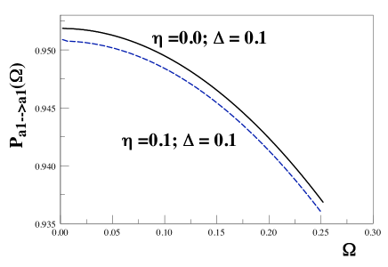
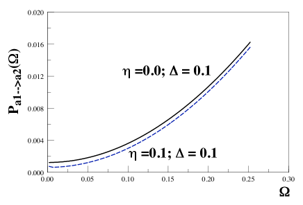
Figure 2: Disappearance and appearance probabilities for $\Delta=0.1$ and $\eta=0,0.1$ to compare canonical and unsterile neutrinos.

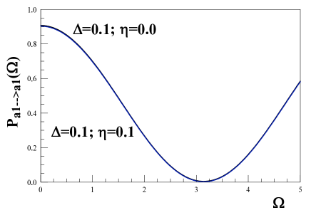
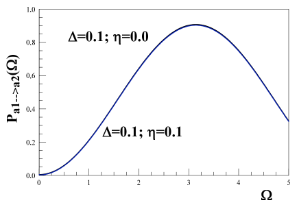
Figure 3: By the first oscillation peak, the difference between canonical sterile and unsterile neutrinos has disappeared.

The discussion above applies in the limit $\Delta\ll 1$ which has been invoked from the beginning to establish a see-saw hierarchy between the active-like and unsterile-like neutrinos. However, the proposal for a “solution” of the LSND/MiniBooNE discrepancy introduces a sterile neutrino in the $eV$ mass range, namely within the same mass range as the active neutrinos. This possibility requires that $\Delta\sim\mathcal{O}(1)$. Although our study does not apply directly to this regime, we can extrapolate to this regime in several aspects.

First, the mixing angle $\Phi_{3}$, which determines the overlap between active-like and unsterile-like modes, becomes of the same order as the angle $\theta$ that determines the overlap between active-like states. This modifies the appearance and disappearance probabilities by overall normalizations. However, the argument on Lorentz invariance still implies, at least within the quantum mechanical description of oscillations, that the angles are evaluated on the mass shell of the single particle states and do not depend on the energy.

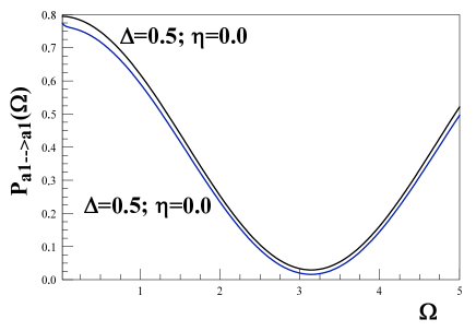
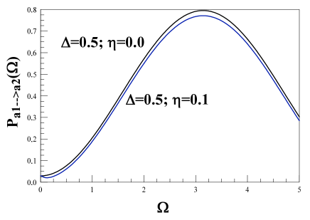
Figure 4: For larger $\Delta$ the suppression effect due to the anomalous dimension is more prominent.

For $\Delta\sim\mathcal{O}(1)$, it follows from Eq. (85) that $\tilde{\Omega}\sim\Omega$ and the oscillation frequencies of both oscillatory terms in the probabilites are of the same order. Furthermore, the factor $\tilde{A}$ of Eq. (74) that determines the interference terms from the threshold of the massive active mode and the unsterile mode become of order $\sin[2\pi\eta]$. Therefore, for $\eta\lesssim 1/3$, but not too small, this overlap yields a potentially interesting energy dependence. In this case, the suppression of the probabilities as a consequence of the anomalous dimension is non-vanishing even for long baseline events, namely with $\Omega\sim\mathcal{O}(1)$. However, for large $\eta$ such that $\tan\pi\eta\sim 1$ and $\Delta\sim\mathcal{O}(1)$, the attenuation length of the overlap (see Eq. (86)) is substantial and the interference between active and unsterile-like is suppressed over the baseline. The appearance and disappearance probabilities for $\Delta=0.5$ are shown in Fig. (4).

IV Summary

In this article, we considered the possibility that the $SU(2)$ singlet sterile neutrino is an unparticle and mixes with the active neutrinos. The unparticle sterile neutrino – or unsterile neutrino – is an interpolating field that describes a multiparticle continuum as a consequence of coupling to a “hidden” conformal sector and whose correlation functions feature an anomalous scaling dimension $\eta$. We analyzed the consequences of its mixing with two active neutrinos via a “minimal” see-saw mass matrix, with massless active neutrinos and no active-active mixing term.

We have introduced a generalization of the usual quantum mechanical description of the dynamics of mixing and oscillation that incorporates the propagators for the fields associated with the mass eigenstates and includes off-shell corrections to the time dependence of the appearance and disappearance probabilities for the active-like neutrinos. We find a remarkable interference phenomenon between the massive active-like and unsterile-like modes as a consequence of threshold effects which modify both appearance and disappearance probabilities in a novel manner.

The presence of the anomalous dimension that gives the unparticle nature to the sterile neutrino has profound consequences in the disappearance and appearance probabilities for the active-like modes. For a canonical sterile neutrino, the disappearance probability is different for the different flavors as a consequence of the fact that the transformation between flavor and mass eigenstates is not unitary in the active sector. This same feature remains in case of the unsterile neutrino, however, the anomalous dimension is responsible for novel time dependent phenomena corresponding to the new oscillatory term arising from the interference of the threshold of the massive active-like mode and the unsterile mode. This oscillatory term is multiplied by an attenuating function of baseline but the oscillation length is different from the active-active one. These novel contributions are consequences of the unparticle nature of the sterile neutrino and result in a suppression of both probabilities on short baseline experiments as compared to the case of active-sterile mixing with a canonical sterile neutrino. Combined analysis of short and long baseline experiments may, therefore, provide a diagnostic tool for the unparticle nature of a sterile neutrino. Another important manifestation of the unparticle nature of the sterile neutrino is the non-vanishing spectral density “inherited” by the massive active mode, which may lead to the possibility of new reaction channels when the standard model interactions are present.

Although these effects would be potentially relevant in the phenomenological reconciliation between the LSND and MiniBooNE data, we find that as a consequence of Lorentz invariance, the mixing angles, when evaluated on the mass shell of the corresponding mass eigenstates do not depend on energy as required for a reconciliation of the dataSchwetz:2007cd . Furthermore, within the simple model considered here, we find that either with a large see-saw hierarchy of masses between the unsterile-like and the active like neutrinos, or even if they all feature the same mass scale, the new interference terms that could be responsible for novel effects are probably too small to reconcile the LSND and MiniBooNE data.

We would like to emphasize that there are, however, some important caveats: the framework introduced as a generalization of the quantum mechanical description of the dynamics of mixing and oscillations can at best be a proxy for a full quantum field theoretical treatment of the appearance and disappearance probabilities in real time in which “flavor” neutrinos are intermediate states, including the propagation of the unsterile degree of freedom. Furthermore, considering either a more realistic $3+\tilde{1}$ scenario or a more general mixing matrix in $2+\tilde{1}$ scheme with mass scales of the same order may provide a scenario in which the novel phenomena found here may yield rich phenomenology. For example, in $2+\tilde{1}$ scheme, giving one of the active neutrinos a mass, which can be acquired by including another type beyond standard model sector, already results in a momentum dependent active-active mixing angle.

Although the simple model studied here may not provide the reconciliation between the LSND and MiniBooNE data, the novel time dependent phenomena that emerges as a consequence of the unparticle nature of the sterile neutrino warrants further and deeper study. We anticipate important cosmological consequences in the equilibration of active neutrinos, novel mechanisms for sterile neutrino production and possibly interesting consequences for light dark matter candidates.

Appendix A Oscillations of bosonic single particle states

Neutrino mixing and oscillations is conventionally studied via a single particle quantum mechanical description. In this formulation, there is no distinction on whether the states of the quantum field theory correspond to fermionic or bosonic particles, and in the case of fermions, there is no mention of helicity or any other quantum numbers besides energy and momentum.

In this appendix, by considering bosonic particles, we study the dynamics of oscillations to establish potential differences with the fermionic case described in the text. Let us consider a mixing of two canonical neutrinos. The mass eigenstates are given by

$$\nu_{1} = \cos\theta\,\nu_{a}+\sin\theta\,\nu_{b},$$ (87)

$$\nu_{2} = \cos\theta\,\nu_{b}-\sin\theta\,\nu_{a}\,,$$ (88)

with $\nu_{a,b}$ are the flavor eigenstates and the masses corresponding to the fields $\nu_{1,2}$ are $M_{1,2}$, respectively. The transition amplitude $|\langle\nu_{a}(t)|\nu_{b}(0)\rangle|^{2}$ is calculated using ordinary quantum mechanics:

$$\langle\nu_{a}(t)|\nu_{b}(0)\rangle=\langle\nu_{a}(t)|\nu_{1}(t)\rangle\,\langle\nu_{1}(t)|\nu_{1}(0)\rangle\,\langle\nu_{1}(0)|\nu_{b}(0)\rangle+\langle\nu_{a}(t)|\nu_{2}(t)\rangle\,\langle\nu_{2}(t)|\nu_{2}(0)\rangle\,\langle\nu_{2}(0)|\nu_{b}(0)\rangle,$$ (89)

where the equal time overlaps $\langle\nu_{a,b}|\nu_{1,2}\rangle$ are read from Eqs. (87) and (88), while the time evolution $\langle\nu_{1,2}(t)|\nu_{1,2}(0)\rangle$ can be obtained from the field theory by considering the time evolution of a single particle state $|1_{\mathbf{k}}\rangle$. To do that, let us first express the field describing the mass eigenstates using the creation and annihilation operators

$$\nu_{j}(\mathbf{k},t=0)=\frac{1}{\sqrt{2E_{j}}}\,\left(a_{\mathbf{k}}+a_{-{\mathbf{k}}}^{\dagger}\right),$$ (90)

where

$$\nu_{j}(\mathbf{x},t=0)=\int\frac{d^{3}k}{\left(2\pi\right)^{3}}\,\nu_{j}(k)\,e^{i\mathbf{k}\cdot\mathbf{x}},$$ (91)

and $E_{j}^{2}=k^{2}+M_{j}^{2}$.

The time evolution $\langle\nu_{1,2}(t)|\nu_{1,2}(0)\rangle$ is then given by

$$\langle\nu_{j}(t)|\nu_{j}(0)\rangle = \langle 1_{\mathbf{k}}|\,e^{-iHt}\,|1_{\mathbf{k}}\rangle$$

$$= 2E_{j}\,\langle 0|\,\nu_{j}(\mathbf{k},t)\,\nu_{j}^{\dagger}(\mathbf{k},t=0)\,|0\rangle$$

$$= 2E_{j}\,\int\frac{dE}{2\pi i}\,e^{-iEt}\,G_{j}(E,\mathbf{k})$$

$$= 2E_{j}\int\frac{dE}{2\pi i}\,\frac{e^{-iEt}}{E^{2}-k^{2}-M_{j}^{2}+i\epsilon}$$

$$= e^{-iE_{j}t}\,.$$ (93)

Therefore the amplitude is

$$|\langle\nu_{a}(t)|\nu_{b}(0)\rangle|^{2} = \sin^{2}2\theta\,\sin^{2}\frac{\left(E_{2}-E_{1}\right)t}{2}$$

$$\Rightarrow|\langle\nu_{a}(L)|\nu_{b}(0)\rangle|^{2} \approx \sin^{2}2\theta\,\sin^{2}\frac{\left(M_{2}^{2}-M_{1}^{2}\right)L}{4k},$$ (94)

where on the second line we have used the ultra-relativistic approximation. Here, L is the length of the baseline used in the experiment.

Let us apply this to the $\tilde{2}+1$-scenario. First of all, the overlaps $\langle\nu_{a_{1,2}}|\nu_{1,2,3}\rangle$ can be derived from Eqs. (18) - (20). Let us start by expressing the energy eigenstates in terms of the “flavor” eigenstates as

$$|\nu_{1}\rangle_{E,k} = -\sin\theta_{E,k}\,|\nu_{a_{1}}\rangle_{k}+\cos\theta_{E,k}\,|\nu_{a_{2}}\rangle_{k}\,,$$ (95)

$$|\nu_{2}\rangle_{E,k} = \cos\phi_{E,k}\,\cos\theta_{E,k}\,|\nu_{a_{1}}\rangle_{k}+\cos\phi_{E,k}\,\sin\theta_{E,k}\,|\nu_{a_{2}}\rangle_{k}-\sin\phi_{E,k}\,|\nu_{U}\rangle_{k}\,,$$ (96)

$$|\nu_{3}\rangle_{E,k} = \sin\phi_{E,k}\,\cos\theta_{E,k}\,|\nu_{a_{1}}\rangle_{k}+\sin\phi_{E,k}\,\sin\theta_{E,k}\,|\nu_{a_{2}}\rangle_{k}+\cos\phi_{E,k}\,|\nu_{U}\rangle_{k}\,,$$ (97)

where we have made explicit the energy and momentum dependence. Since we are using one-particle quantum mechanics to describe the system, the energy eigenstates must be evaluated on-shell. Therefore

$$|\nu_{1}\rangle = -\sin\theta\,|\nu_{a_{1}}\rangle+\cos\theta\,|\nu_{a_{2}}\rangle\,,$$ (98)

$$|\nu_{2}\rangle = \cos\Phi_{2}\,\cos\theta\,|\nu_{a_{1}}\rangle+\cos\Phi_{2}\,\sin\theta\,|\nu_{a_{2}}\rangle-\sin\Phi_{2}\,|\nu_{U}\rangle\,,$$ (99)

$$|\nu_{3}\rangle = \sin\Phi_{3}\,\cos\theta\,|\nu_{a_{1}}\rangle+\sin\Phi_{3}\,\sin\theta\,|\nu_{a_{2}}\rangle+\cos\Phi_{3}\,|\nu_{U}\rangle\,,$$ (100)

where $\phi_{i}$ means that the angle $\phi$ is evaluated at $p^{2}={\cal M}_{i}^{2}$, and we have dropped the index for the angle $\theta$ as it is a constant and does not depend on the four-momentum. We note that $\sin\phi_{3}$ and $\cos\phi_{3}$ are complex as ${\cal M}_{3}>M$. Here, we have also dropped the indices on the states to simplify the notation. We can then solve Eqs. (98) - (100) for the “flavor” eigenstates to obtain the overlaps.

Next, we need the time evolution of the mass eigenstates $\langle\nu_{i}(t)|\nu_{i}(0)\rangle$, especially for $i=2,3$. We can obtain these by substituting their respective propagators into Eq. (A) and it is convenient to use the dispersive form of the propagators Bjorken:1979dk . The time evolution is then given by

$$S_{2} \equiv \langle\nu_{2}(t)|\nu_{2}(0)\rangle$$ (101)

$$= \int_{0}^{\infty}dQ^{2}\,\rho_{2}(Q^{2})\,e^{-i\sqrt{k^{2}+Q^{2}}\,t}$$

$$= Z_{2}\,e^{-iE_{2}t}+e^{-iE_{M}t}\int_{0}^{\infty}dx\,\rho_{2}(x)\,\exp\left[-i\,\frac{M^{2}}{E_{M}}t\,x\right],$$

where we have introduced $E_{M}(k)=\sqrt{k^{2}+{M}^{2}}$, and $x$ is the dimensionless variable defined in Eq. (24).

For the case of $\nu_{2}$, since the pole is below the continuum, we can estimate the large time behavior of $S_{2}$ by replacing $\rho_{2}$ with its near-threshold behavior. Therefore

$$S_{2} = Z_{2}\,e^{-iE_{2}(k)t}+\frac{\Delta^{2}}{4\pi}\,\sin(2\pi\eta)\,e^{-iE_{M}(k)t}\int_{0}^{\infty}dx\,x^{2\eta}\,\exp\left[-i\,\frac{M^{2}}{E_{M}}t\,x\right]$$ (102)

$$= Z_{2}\,e^{-iE_{2}t}+\frac{A_{2}}{i^{1+2\eta}}\,\left(\frac{E_{M}}{M^{2}\,t}\right)^{1+2\eta}\,e^{-iE_{M}t}\,,$$

with

$$A_{2}=\frac{\Delta^{2}}{4\pi}\,\sin(2\pi\eta)\,\Gamma(1+2\eta)\,.$$ (103)

For $\nu_{3}$, we can estimate $S_{3}$ by approximating the spectral density by a Breit-Wigner Lorentzian, (see Eq. (27)) from which we obtain

$$S_{3} = Z_{3}\,e^{-iE_{3}(k)t}\,e^{-\frac{\Gamma}{2\gamma}t},$$ (104)

where $\Gamma$ is the decay width given by Eq. (30) and $\gamma=E_{3}(k)/\mathcal{M}_{3}$ is the Lorentz factor.

Finally, by combining all the results above, we find that at large time

$$|\langle\nu_{a_{2}}(t)|\nu_{a_{1}}(0)\rangle|^{2} = \frac{\sin^{2}2\theta}{4}\Bigg{\{}1+\cos^{4}\Phi_{2}\left[Z_{2}^{2}+A_{2}^{2}\left(\frac{E_{M}}{M^{2}\,t}\right)^{2+4\eta}\right]-2\,Z_{2}\,\cos^{2}\Phi_{2}\,\cos\big{[}(E_{2}-E_{1})\,t\big{]}$$ (105)

$$+\,2\,A_{2}\,Z_{3}\,\cos^{2}\Phi_{2}\,|\sin\Phi_{3}|^{2}\,e^{-\frac{\Gamma}{2\gamma}t}\,\left(\frac{E_{M}}{M^{2}\,t}\right)^{1-\eta}\,\cos\big{[}(E_{3}-E_{M})t-\frac{\pi}{2}(1+2\eta)\big{]}$$

$$+\,Z_{3}^{2}\,|\sin\Phi_{3}|^{4}e^{-\frac{\Gamma}{\gamma}t}\Bigg{\}}$$

$$\Rightarrow|\langle\nu_{a_{2}}(L)|\nu_{a_{1}}(0)\rangle|^{2} \approx \frac{\sin^{2}2\theta}{4}\Bigg{\{}1+\cos^{4}\Phi_{2}\left[Z_{2}^{2}+A_{2}^{2}\left(\frac{E_{M}}{M^{2}\,L}\right)^{2+4\eta}\right]-2\,Z_{2}\,\cos^{2}\Phi_{2}\,\cos\left[\frac{{\cal M}_{2}^{2}\,L}{2k}\right]$$ (106)

$$+\,2\,A_{2}\,Z_{3}\,\cos^{2}\Phi_{2}\,|\sin\Phi_{3}|^{2}\,e^{-\frac{\Gamma}{2\gamma}L}\,\left(\frac{E_{M}}{M^{2}\,L}\right)^{1-\eta}\,\cos\left[\frac{({\cal M}_{3}^{2}-M^{2})\,L}{2k}-\frac{\pi}{2}(1+2\eta)\right]\,$$

$$+\,Z_{3}^{2}\,|\sin\Phi_{3}|^{4}e^{-\frac{\Gamma}{\gamma}L}\Bigg{\}}\,,$$

where in going from Eq. (105) to Eq. (106) we have used the ultra-relativistic approximation and replaced $t$ by the baseline $L$.

References

- (1) R. N. Mohapatra and P. B. Pal, “Massive neutrinos in physics and astrophysics. Second edition,” World Sci. Lect. Notes Phys. 60, 1 (1998) [World Sci. Lect. Notes Phys. 72, 1 (2004)].
- (2) V. G. Sinitsyna, M. Masip, S. I. Nikolsky and V. Y. Sinitsyna, arXiv:0903.4654 [hep-ph].
- (3) A. A. Aguilar-Arevalo et al. [The MiniBooNE Collaboration], Phys. Rev. Lett. 98, 231801 (2007) [arXiv:0704.1500 [hep-ex]].
- (4) M. Maltoni and T. Schwetz, Phys. Rev. D 76, 093005 (2007) [arXiv:0705.0107 [hep-ph]].
- (5) S. N. Gninenko, arXiv:0902.3802 [hep-ph].
- (6) H. Georgi, Phys. Rev. Lett. 98, 221601 (2007) [arXiv:hep-ph/0703260]; H. Georgi, Phys. Lett. B 650, 275 (2007) [arXiv:0704.2457 [hep-ph]].
- (7) T. Banks and A. Zaks, Nucl. Phys. B 196, 189 (1982).
- (8) P. J. Fox, A. Rajaraman and Y. Shirman, Phys. Rev. D 76, 075004 (2007) [arXiv:0705.3092 [hep-ph]].
- (9) K. Cheung, W. Y. Keung and T. C. Yuan, Phys. Rev. Lett. 99, 051803 (2007) [arXiv:0704.2588 [hep-ph]]; A. Arhrib, K. Cheung, C. W. Chiang and T. C. Yuan, Phys. Rev. D 73, 075015 (2006) [arXiv:hep-ph/0602175]; for a recent review see: K. Cheung, W. Y. Keung and T. C. Yuan, AIP Conf. Proc. 1078, 156 (2009) [arXiv:0809.0995 [hep-ph]].
- (10) M. Luo and G. Zhu, Phys. Lett. B 659, 341 (2008) [arXiv:0704.3532 [hep-ph]]; Y. Liao, Phys. Lett. B 665, 356 (2008) [arXiv:0804.0752 [hep-ph]]; R. Basu, D. Choudhury and H. S. Mani, arXiv:0803.4110 [hep-ph].
- (11) B. Grinstein, K. A. Intriligator and I. Z. Rothstein, Phys. Lett. B 662, 367 (2008) [arXiv:0801.1140 [hep-ph]].
- (12) Y. Liao and J. Y. Liu, Phys. Rev. Lett. 99, 191804 (2007) [arXiv:0706.1284 [hep-ph]].
- (13) R. Zwicky, J. Phys. Conf. Ser. 110, 072050 (2008) [arXiv:0710.4430 [hep-ph]].
- (14) Y. f. Wu and D. X. Zhang, arXiv:0712.3923 [hep-ph]; R. Mohanta and A. K. Giri, Phys. Rev. D 76, 057701 (2007) [arXiv:0707.3308 [hep-ph]]; J. K. Parry, arXiv:0810.0971 [hep-ph].
- (15) G. J. Ding and M. L. Yan, Phys. Rev. D 78, 075015 (2008) [arXiv:0706.0325 [hep-ph]]; G. Bhattacharyya, D. Choudhury and D. K. Ghosh, Phys. Lett. B 655, 261 (2007) [arXiv:0708.2835 [hep-ph]].
- (16) C. M. Ho and Y. Nakayama, JHEP 0905, 081 (2009) [arXiv:0903.0420 [hep-th]].
- (17) S. Hannestad, G. Raffelt and Y. Y. Y. Wong, Phys. Rev. D 76, 121701 (2007) [arXiv:0708.1404 [hep-ph]].
- (18) N. G. Deshpande, S. D. H. Hsu and J. Jiang, Phys. Lett. B 659, 888 (2008) [arXiv:0708.2735 [hep-ph]].
- (19) A. Freitas and D. Wyler, JHEP 0712, 033 (2007) [arXiv:0708.4339 [hep-ph]].
- (20) J. McDonald, arXiv:0805.1888 [hep-ph]; JCAP 0903, 019 (2009) [arXiv:0709.2350 [hep-ph]].
- (21) H. Davoudiasl, Phys. Rev. Lett. 99, 141301 (2007) [arXiv:0705.3636 [hep-ph]].
- (22) I. Lewis, arXiv:0710.4147 [hep-ph].
- (23) G. L. Alberghi, A. Y. Kamenshchik, A. Tronconi, G. P. Vacca and G. Venturi, Phys. Lett. B 662, 66 (2008) [arXiv:0710.4275 [hep-th]].
- (24) S. L. Chen, X. G. He, X. P. Hu and Y. Liao, Eur. Phys. J. C 60, 317 (2009) [arXiv:0710.5129 [hep-ph]].
- (25) T. Kikuchi and N. Okada, Phys. Lett. B 665, 186 (2008) [arXiv:0711.1506 [hep-ph]], Phys. Lett. B 661, 360 (2008) [arXiv:0707.0893 [hep-ph]], Phys. Rev. D 77, 094012 (2008) [arXiv:0801.0018 [hep-ph]].
- (26) Y. Gong and X. Chen, Eur. Phys. J. C 57, 785 (2008) [arXiv:0803.3223 [astro-ph]].
- (27) H. Collins and R. Holman, Phys. Rev. D 78, 025023 (2008) [arXiv:0802.4416 [hep-ph]].
- (28) D. Boyanovsky, R. Holman and J. A. Hutasoit, Phys. Rev. D 79, 085018 (2009) [arXiv:0812.4723 [hep-ph]].
- (29) X. Q. Li, Y. Liu and Z. T. Wei, Eur. Phys. J. C 56, 97 (2008) [arXiv:0707.2285 [hep-ph]].
- (30) S. Zhou, Phys. Lett. B 659, 336 (2008) [arXiv:0706.0302 [hep-ph]].
- (31) G. Gonzalez-Sprinberg, R. Martinez and O. A. Sampayo, Phys. Rev. D 79, 053005 (2009) [arXiv:0808.1747 [hep-ph]].
- (32) D. Boyanovsky, R. Holman and J. A. Hutasoit, Phys. Rev. D 80, 025012 (2009) [arXiv:0905.4729 [hep-ph]].
- (33) T. Schwetz, JHEP 0802, 011 (2008) [arXiv:0710.2985 [hep-ph]].
- (34) A. Aguilar et.al. (LSND collaboration), Phys. Rev. D 64, 112007 (2001) [arXiv:hep-ex/0104049].
- (35) D. Boyanovsky and C. M. Ho, Phys. Rev. D 69, 125012 (2004) [arXiv:hep-ph/0403216].
- (36) C. M. Ho, D. Boyanovsky and H. J. de Vega, Phys. Rev. D 72, 085016 (2005) [arXiv:hep-ph/0508294]; C. M. Ho and D. Boyanovsky, Phys. Rev. D 73, 125014 (2006) [arXiv:hep-ph/0604045].
- (37) J. Wu, C. M. Ho and D. Boyanovsky, Phys. Rev. D80, 103511 (2009) arXiv:0902.4278 [hep-ph]
- (38) J. Wu, J. A. Hutasoit, D. Boyanovsky and R. Holman, arXiv:1002.2649 [hep-ph].
- (39) J. D. Bjorken and S. D. Drell, Relativistic Quantum Field Theory , (McGraw-Hill, N.Y. 1965).
- (40) L. S. Brown, Quantum Field Theory, (Cambridge University Press, Cambridge, 1994).