Energetics and performance of a microscopic heat engine based on exact calculations of work and heat distributions

Abstract

We investigate a microscopic motor based on an externally controlled two-level system. One cycle of the motor operation consists of two strokes. Within each stroke, the two-level system is in contact with a given thermal bath and its energy levels are driven with a constant rate. The time evolution of the occupation probabilities of the two states are controlled by one rate equation and represent the system’s response with respect to the external driving. We give the exact solution of the rate equation for the limit cycle and discuss the emerging thermodynamics: the work done on the environment, the heat exchanged with the baths, the entropy production, the motor’s efficiency, and the power output. Furthermore we introduce an augmented stochastic process which reflects, at a given time, both the occupation probabilities for the two states and the time spent in the individual states during the previous evolution. The exact calculation of the evolution operator for the augmented process allows us to discuss in detail the probability density for the performed work during the limit cycle. In the strongly irreversible regime, the density exhibits important qualitative differences with respect to the more common Gaussian shape in the regime of weak irreversibility.

1 Introduction

Non-equilibrium phenomena in the presence of time-varying external fields are of vital interest in many areas of current research [1, 2, 3]. Examples are aging and rejuvenation effects in the rheology of soft-matter systems and in the dynamics of spin glasses, relaxation and transport processes in biological systems such as molecular motors, ion diffusion through membranes, or stretching of DNA molecules, driven diffusion systems with time-dependent bias, and nano-engines. With minimization of the system size thermal fluctuations become increasingly relevant. In these systems it is useful to introduce microscopic heat and work quantities as random variables whose averages yield the common thermodynamic quantities. Averages over functions of these microscopic heat and work quantities yield generalized fluctuation theorems [4, 5, 6, 7, 8, 9, 10, 11, 12, 13, 14]. In this context mesoscopic engines operating between different heat baths under non-equilibrium conditions have received increasing attention. The variety of models can be roughly classified according to the dynamical laws involved. In the case of the classical stochastic heat engines, the state space can either be discrete or continuous (c.f., for example, [15, 16, 17] and the references therein). Examples of the quantum heat engines are studied, e.g., in [18, 19].

The traditional consideration of efficiency of heat engines operating between two baths at temperatures $T_{1}$ and $T_{2}$ leads to the Carnot upper bound $\eta_{\rm C}=1-T_{1}/T_{2}$. The bound is only achieved under reversible conditions where the state changes require infinite time and hence the power output is zero. Real heat engines generate a finite power output $P_{\mathrm{out}}=W_{\mathrm{out}}/t_{{\rm cycle}}$, i.e., they perform work $W_{\mathrm{out}}$ during a cycle of a finite duration $t_{{\rm cycle}}$. Thus an appropriate way to characterize the engines is to compare their efficiencies at maximum power. On the macroscopic level this quantity is roughly bounded by the Curzon-Ahlborn value $\eta_{\rm CA}=1-\sqrt{T_{1}/T_{2}}$ [20]. Alternative expressions for quantifying efficiency have been discussed [17] which are based on mean quantities, e.g., on the mean work done during the operational cycle. On the mesoscopic level, the work is inherently a fluctuating quantity and one should be able to calculate not only its mean value but also its fluctuation properties.

In this paper we study a simple model of mesoscopic heat engines operating between two different heat baths under non-equilibrium conditions. The working medium consist of a two-level system. The cycle of operation includes just two isothermal branches, or strokes. Within each stroke, the system is driven by changing the energies of the two states and we assume a constant driving rate, i.e. a linear time-dependence of the energies. The response of the working medium is governed by a master equation with time-dependent transition rates. The specific form of the rates guarantees that, provided the two energies were fixed, the system would relax towards the Gibbs equilibrium state. Of course, during the motor operation, the Gibbs equilibrium is never achieved because the energies are cyclically modulated. At a given instant, the system’s dynamics just reflects the instantaneous position of the energy levels. After a transient regime, the engine dynamics approaches limit cycle with the periodicity of the driving force. We will focus on the properties of this limit cycle. In particular, we calculate the distribution of the work during the limit cycle.

Our two-isotherm setting imposes one important feature which is worth emphasizing. As stated above, at the end of each branch we remove the present bath and we allow the thermal interaction with another reservoir. This exchange of reservoirs necessarily implies a finite difference between the new reservoir temperature and the actual system (effective) temperature. Even if the driving period tends to infinity, we shall observe a positive entropy production originating from the relaxation processes initiated by the abrupt change of the contact temperature. Differently speaking, our engine operates in an inherently irreversible way and there exists no reversible limit.

The paper is organized as follows. In section 2 we solve the dynamical equation for the externally driven working medium. For the sake of clarity we first give the solution just for an unrestricted linear driving protocol using a generic driving rate and a generic reservoir (section 2.1). Thereupon, in section 2.2, we particularize the generic solution to individual branches and, using the Chapman-Kolmogorov condition, we derive the solution for the limit cycle. In section 3 we employ the recently derived [21] analytical result for the work probability density under linear driving. Again, we first give the result for the generic linear driving and then we combine two such particular solutions into the final work distribution valid for the limit cycle. The results from section 2 and section 3 enable a detailed calculation of the energy and entropy flows during the limit cycle in section 4 and allow for a discussion of the engine performance in section 5.

2 Description of the engine and its limit cycle

Consider a two-level system with time-dependent energies $E_{i}(t)$, $i=1,2$, in contact with a single thermal reservoir at temperature $T$. In general, the heat reservoir temperature $T$ may also be time-dependent. The time evolution of the occupation probabilities $p_{i}(t)$, $i=1,2$, is governed by the master equation [22] with time-dependent transition rates specified by the reservoir temperature and by the external parameters. To be specific the dynamics of the system is described by the time inhomogeneous Markov process $\mathsf{D}(t)$ assuming the value $i$, $i=1,2$, if the system resides at time $t$ in the $i$th state. Explicitly, the master equation reads

$$\frac{\mathrm{d}}{\mathrm{d}t}\mathbb{R}(t\,|\,t^{\prime})=-\left(\begin{array}[]{rr}\lambda_{1}(t)&-\lambda_{2}(t)\\ -\lambda_{1}(t)&\lambda_{2}(t)\end{array}\right)\,\mathbb{R}(t\,|\,t^{\prime})\,\,,\qquad\mathbb{R}(t^{\prime}\,|\,t^{\prime})=\mathbb{I}\,,$$ (1)

where $\mathbb{I}$ is the unity matrix and ${\mathbb{R}}(t,t^{\prime})$ the transition matrix with elements $R_{ij}(t\,|\,t^{\prime})=\langle\,i\,|\,{\mathbb{R}}(t\,|\,t^{\prime})\,|\,j\,\rangle$, $i,j=1,2$. These elements are the conditional probabilities

$$R_{ij}(t\,|\,t^{\prime})={\rm Prob}\left\{\,\mathsf{D}(t)=i\,|\,\mathsf{D}(t^{\prime})=j\,\right\}\,.$$ (2)

If we denote by $\phi(t^{\prime})$ the initial state at time $t^{\prime}$ with the occupation probabilities $p_{i}(t^{\prime})=\left\langle\,i\,|\phi(t^{\prime})\right\rangle$, the occupation probabilities at the observation time $t$ are described by the column vector $\left|p(t,t^{\prime})\right\rangle=\mathbb{R}(t\,|\,t^{\prime})\,\left|\phi(t^{\prime})\right\rangle$.

Due to the conservation of the total probability the system (1) can be reduced to just one non-homogeneous linear differential equation of the first order. Therefore the master equation (1) is exactly solvable for arbitrary functions $\lambda_{1}(t)$, $\lambda_{2}(t)$. The rates are typically a combination of an attempt frequency to exchange the state multiplied by an acceptance probability. We shall adopt the Glauber form

$$\lambda_{1}(t)=\frac{\nu}{1+\exp\left\{-\beta(t)\left[E_{1}(t)-E_{2}(t)\right]\right\}}\,,\;\lambda_{2}(t)=\lambda_{1}(t)\exp\left\{-\beta(t)\left[E_{1}(t)-E_{2}(t)\right]\right\},$$ (3)

where $\nu^{-1}$ sets the elementary time scale, and $\beta(t)=1/k_{B}T(t)$. The rates in equation (1) satisfy the (time local) detailed balance condition.

The general solution of the master equation (1) for the transfer rates (3) reads

$$\mathbb{R}(t\,|\,t^{\prime})=\mathbb{I}-\frac{1}{2}\left(\begin{array}[]{rr}1&-1\\ -1&1\end{array}\right)\left\{1-\exp\left[-\nu(t-t^{\prime})\right]\right\}+\frac{1}{2}\left(\begin{array}[]{rr}-1&-1\\ 1&1\end{array}\right)\,\xi(t,t^{\prime})\,,$$ (8)

where

$$\xi(t,t^{\prime})=\nu\int_{t^{\prime}}^{t}\,\mathrm{d}\tau\,\exp\left[-\nu(t-\tau)\right]\,\tanh\left\{\frac{\beta(\tau)}{2}\,\left[E_{1}(\tau)-E_{2}(\tau)\right]\right\}\,.$$ (9)

The resulting propagator satisfies the Chapman-Kolmogorov condition

$$\mathbb{R}(t\,|\,t^{\prime})=\mathbb{R}(t\,|\,t^{\prime\prime})\mathbb{R}(t^{\prime\prime}\,|\,t^{\prime})$$ (10)

for any intermediate time $t^{\prime\prime}$. Its validity can be easily checked by direct matrix multiplication. The condition simply states that the initial state for the evolution in the time interval $[t^{\prime\prime},t]$ can be taken as the final state reached in the interval $[t^{\prime},t^{\prime\prime}]$. This is true even if the parameters of the process in the second interval differ from those in the first one. Of course, if this is the case, we should use an appropriate notation which distinguishes the two corresponding propagators. This procedure will be actually implemented in the paper. Keeping in mind this possibility, we shall first analyze the propagator for a generic linear driving protocol.

2.1 Generic case – linear driving protocol

Let us consider the linear driving protocol $E_{1}(t)=h+v(t-t^{\prime})$, and $E_{2}(t)=-E_{1}(t)$, where $h=E_{1}(0)$ denotes the energy of the first level at the initial time $t^{\prime}$, and $v$ is the driving velocity (energy change per time). The rates (3) can then be written in the form

$$\lambda_{1}(t)=\nu\frac{1}{1+c\exp[-\Omega(t-t^{\prime})]}\,,\,\,\,\,\lambda_{2}(t)=\nu\frac{c\exp[-\Omega(t-t^{\prime})]}{1+c\exp[-\Omega(t-t^{\prime})]}\,,$$ (11)

where $\Omega=2\beta|v|$ is the temperature-reduced driving velocity, and $c=\exp(-2\beta h|v|/v)$ incorporates the initial values of the energies.

Under this linear driving protocol one can evaluate the definite integral in (8) explicitly and rewrite the propagator as

$$\mathbb{R}(t\,|\,t^{\prime})=\mathbb{I}-\left(\begin{array}[]{cc}\phantom{-}1&\phantom{-}0\\ -1&\phantom{-}0\end{array}\right)\left\{1-\exp{\left[-\nu(t-t^{\prime})\right]}\right\}+\left(\begin{array}[]{cc}\phantom{-}1&\phantom{-}1\\ -1&-1\end{array}\right)\gamma(t,t^{\prime})\,,$$ (16)

where

$$\gamma(t,t^{\prime}) = \nu\,c\int_{t^{\prime}}^{t}\,\mathrm{d}\tau\,\exp{\left[-\nu(t-\tau)\right]}\frac{\exp{\left(-\Omega\tau\right)}}{1+c\exp{\left(-\Omega\tau\right)}}$$ (17)

$$= a\,c\exp{\left(-\nu t\right)}\int_{\Omega t^{\prime}}^{\Omega t}\mathrm{d}\tau\,\frac{\exp{\left[(a-1)\tau\right]}}{1+c\exp{\left(-\tau\right)}}\,.$$

Here we have introduced the dimensionless ratio $a=\nu/\Omega$ of the attempt frequency characterizing the time scale of the system’s dynamics and the time scale of the external driving, respectively. Naturally, this ratio will describe the degree of irreversibility of the process. Depending on the value $a\in(0,\infty)$, the explicit form of the function $\gamma(t,t^{\prime})$ reads

$$\gamma(t,t^{\prime})=\left\{\begin{array}[]{ll}\frac{ac}{1-a}\exp{\left(-\nu t\right)}\left\{\exp{\left[(a-1)\Omega t^{\prime}\right]}\,\mathrm{{}_{2\,}\!F\!_{1}}(1,1-a;2-a;-c\exp{\left(-\Omega t^{\prime}\right)})\right.&\\[4.30554pt] \left.\hskip 5.69046pt-\exp{\left[(a-1)\Omega t\right]}\,\mathrm{{}_{2\,}\!F\!_{1}}(1,1-a;2-a;-c\exp{\left(-\Omega t\right)})\right\}\,,&a\in(0,1)\,,\\[8.61108pt] c\exp{\left(-\Omega t\right)}\left[\Omega(t-t^{\prime})+\ln{\displaystyle\frac{1+c\exp{\left(-\Omega t\right)}}{1+c\exp{\left(-\Omega t^{\prime}\right)}}}\right]\,,&a=1\,,\\[8.61108pt] \hskip 5.69046pt\mathrm{{}_{2\,}\!F\!_{1}}(1,a;1+a;-\frac{1}{c}\exp{\left(\Omega t\right)})&\\[4.30554pt] -\exp{\left[-a\Omega(t-t^{\prime})\right]}\,\mathrm{{}_{2\,}\!F\!_{1}}(1,a;1+a;-\frac{1}{c}\exp{\left(\Omega t^{\prime}\right)})\,,&a>1\,,\end{array}\right.$$ (23)

where $\mathrm{{}_{2\,}\!F\!_{1}}(\alpha,\beta;\gamma;\cdot)$ denotes the Gauss hypergeometric function [23].

2.2 Piecewise linear periodic driving

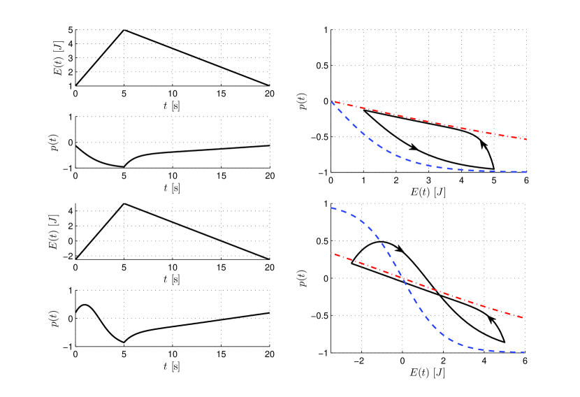
We now introduce the setup for the operational cycle of the engine under periodic driving. Within a given period, two branches with linear time-dependence of the state energies are considered with different velocities. Starting from the value $h_{1}$, the energy $E_{1}(t)$ linearly increases in the first branch until it attains the value $h_{2}>h$, at time $t_{+}$ and in the second branch, the energy $E_{1}(t)$ linearly decreases towards its original value $h_{1}$ in a time $t_{-}$ (see figure 1). We always assume $E_{2}(t)=-E_{1}(t)$, i.e.

$$E_{1}(t)=-E_{2}(1)=\left\{\begin{array}[]{ll}h_{1}+\frac{\displaystyle h_{2}-h_{1}}{\displaystyle t_{+}}\,t\,,&t\in\left[0,t_{+}\right]\,,\\[4.30554pt] h_{2}-\frac{\displaystyle h_{2}-h_{1}}{\displaystyle t_{-}}\,(t-t_{+})\,,&t\in\left[t_{+},t_{+}+t_{-}\right]\,\,.\end{array}\right.$$ (24)

This pattern will be periodically repeated, the period being $t_{\rm p}=t_{+}+t_{-}$.

As the second ingredient, we need to specify the temperature schedule. The two-level system will be alternately exposed to a hot and a cold reservoir, which means that the function $\beta(t)$ in equation (3) will be a piecewise constant periodic function. During the first branch, it assumes the value $\beta_{+}$, during the second branch it attains the value $\beta_{-}$.

This completes the description of the model. Any quantity describing the engine’s performance can only depend on the parameters $h_{1}$, $h_{2}$, $\beta_{\pm}$, $t_{\pm}$, and $\nu$. In the following we will focus on the characterization of the limit cycle, which the engine will approach at long times after a transient period.

We start from the general solution (8) of the master equation (1). Owing to the Chapman-Kolmogorov condition (10), the propagator within the cycle is

$$\mathbb{R}_{\mathrm{p}}(t)=\left\{\begin{array}[]{ll}\mathbb{R}_{+}(t)\,,&t\in\left[0,t_{+}\right]\,,\\[4.30554pt] \mathbb{R}_{-}(t)\mathbb{R}_{+}(t_{+})\,,&t\in\left[t_{+},t_{\mathrm{p}}\right]\,.\end{array}\right.$$ (25)

Here the matrixes $\mathbb{R}_{\pm}(t)$ evolve the state vector within the respective branches and have the form

$$\mathbb{R}_{+}(t)=\mathbb{I}-\frac{1}{2}\left(\begin{array}[]{cc}\phantom{-}1&-1\\ -1&\phantom{-}1\end{array}\right)\left[1-\exp{\left(-\nu t\right)}\right]+\frac{1}{2}\left(\begin{array}[]{cc}-1&-1\\ \phantom{-}1&\phantom{-}1\end{array}\right)\xi_{+}(t)\,,$$ (30)

$$\mathbb{R}_{-}(t)=\mathbb{I}-\frac{1}{2}\left(\begin{array}[]{cc}\phantom{-}1&-1\\ -1&\phantom{-}1\end{array}\right)\left\{1-\exp{\left[-\nu(t-t_{+})\right]}\right\}+\frac{1}{2}\left(\begin{array}[]{cc}-1&-1\\ \phantom{-}1&\phantom{-}1\end{array}\right)\xi_{-}(t)\,,$$ (35)

where

$$\xi_{+}(t)=\nu\int_{0}^{t}\mathrm{d}\tau\,\exp{\left[-\nu(t-\tau)\right]}\tanh{\left\{\beta_{+}\bigg{[}h_{1}+\frac{h_{2}-h_{1}}{t_{+}}\tau\bigg{]}\right\}}\,,$$ (36)

$$\xi_{-}(t)=\nu\int_{t_{+}}^{t}\mathrm{d}\tau\,\exp{\left[-\nu(t-\tau)\right]}\tanh{\left\{\beta_{-}\bigg{[}h_{2}-\frac{h_{2}-h_{1}}{t_{-}}(\tau-t_{+})\bigg{]}\right\}}\,.$$ (37)

Notice, both propagators $\mathbb{R}_{+}(t)$ and $\mathbb{R}_{-}(t)$ are given by the generic propagator (8). In order to get $\mathbb{R}_{+}(t)$, we replace in equation (9) the initial position of the first energy $h$ by $h_{1}$, the driving velocity $v$ by $v_{+}=(h_{2}-h_{1})/t_{+}$, and we set $t^{\prime}=0$. Analogously, the propagator $\mathbb{R}_{-}(t)$ follows from the generic propagator, if we replace $h$ by $h_{2}$, $v$ by $v_{-}=(h_{1}-h_{2})/t_{-}$, and $t^{\prime}$ by $t_{+}$.

Figure 1: The limit cycle for the two-stroke engine. The three graphs in the upper panel illustrate the case where $h_{2}>h_{1}>0$ and the energy levels do not cross during their driving. On the left side we show $E(t)=E_{1}(t)=-E_{2}(t)$ and the response $p(t)=p_{1}(t)-p_{2}(t)$. On the right hand side the parametric plot of the limit cycle in the $p\!-\!\!E$ plane is displayed. The cycle starts in the upper vertex and proceeds counterclockwise, c.f. the arrows. The dashed and the dot-dashed curves show the equilibrium isotherms corresponding to the baths during the first and the second stroke, respectively. The parameters are: $h_{1}=1\;\mathrm{J}$, $h_{2}=5\;\mathrm{J}$, $t_{+}=5\;\mathrm{s}$, $t_{-}=15\;\mathrm{s}$, $\beta_{+}=0.5\;\mathrm{J}^{-1}$, $\beta_{-}=0.1\;\mathrm{J}^{-1}$, $\nu=1\;\mathrm{s}^{-1}$. The three graphs in the lower panel depict the case where $h_{1}<0<h_{2}$ and the energies cross twice during the cycle. Except $h_{1}=-2.5\;\mathrm{J}$, all parameters are as above.

The system state probabilities at the ends of the periods form a Markov chain and we are interested in its fixed point behavior. If we take the stationary state as the initial condition, the system revisits this special state at the end of the limit cycle. Therefore it suffices to solve the eigenvalue problem $\mathbb{R}_{-}(t_{-})\mathbb{R}_{+}(t_{+})\,\left|p^{{\rm stat}}\right\rangle=\left|p^{{\rm stat}}\right\rangle$. Solving the algebraic equation, the fixed point probabilities $p_{i}^{\rm stat}$ at the beginning (or end) of the limit cycle are

$$p_{1}^{\rm stat}=1-p_{2}^{\rm stat}=\frac{1}{2}\left[1-\frac{\xi_{+}(t_{+})\exp\left(-\nu t_{-}\right)+\xi_{-}(t_{-})}{1-\exp\left(-\nu t_{{\rm p}}\right)}\right].$$ (38)

These probabilities, and hence also the specific form of the limit cycle, depend solely on the model parameters.

We now put aside the transitory regime and we focus entirely on the limit cycle. Generally speaking, the parametric plot of the occupation difference $p(t)\equiv p_{1}(t)-p_{2}(t)$ (the response) versus the energy of the first level $E_{1}(t)$ (the driving) exhibits two possible forms which are exemplified in figure 1. First, we have a one-loop form which is oriented either clockwise or anticlockwise. For clockwise orientation, the work done by the engine on the environment during the limit cycle is negative, while for counter-clockwise orientation it is positive. Secondly, we can obtain a two-loops shape exhibiting again either positive or negative work on the environment. Slowing down the driving, the branches gradually approach the corresponding equilibrium isotherms $p_{\pm}(E)=-\tanh(\beta_{\pm}E/2)$. We postpone the further discussion to the section 4.

3 Probability densities for work and heat

Heuristically, the underlying time-inhomogeneous Markov process $\mathsf{D}(t)$ can be conceived as an ensemble of individual realizations (sample paths). A realization is specified by a succession of transitions between the two states. If we know the number $n$ of the transitions during a path and the times $\{t_{k}\}_{k=1}^{n}$ at which they occur, we can calculate the probability that this specific path will be generated. A given paths yields a unique value of the microscopic work done on the system. For example, if the system is known to remain during the time interval $[t_{k},t_{k+1}]$, $t_{k+1}\geq t_{k}$, in the $i$th state, the work done on the system during this time interval is simply $E_{i}(t_{k+1})-E_{i}(t_{k})$. Accordingly the probability of the paths gives the probability of the work. Viewed in this way, the work itself is a stochastic process and we denote it as $\mathsf{W}(t)$. We are interested in its probability density $\rho(w,t)=\langle\,\delta(\mathsf{W}(t)-w)\,\rangle$, where $\langle\,\ldots\,\rangle$ denotes an average over all possible paths.

As a technical tool we introduce the augmented process $\left\{\mathsf{W}(t),\,\mathsf{D}(t)\right\}$ which simultaneously reflects both the work variable and the state variable of the Markov process. The augmented process is again a time non-homogeneous Markov process. Actually, if we know at a fixed time $t^{\prime}$ both the present state variable $j$ and the work variable $w^{\prime}$, then the subsequent probabilistic evolution of the state and work is completely determined. The work done during a time period $[t^{\prime},t]$, where $t>t^{\prime}$, simply adds to the present work $w^{\prime}$ and it only depends on the succession of the states after the time $t^{\prime}$. And this succession by itself, as we know from section 2, cannot depend on the dynamics before time $t^{\prime}$.

The one-time properties of the augmented process will be described by the functions

$$G_{ij}(w,t\,|\,w^{\prime},t^{\prime})=\lim_{\epsilon\rightarrow 0}\frac{{\rm Prob}\left\{\,\mathsf{W}(t)\in(w,w+\epsilon)\,{\rm and}\,\mathsf{D}(t)=i\,|\,\mathsf{W}(t^{\prime})=w^{\prime}\,{\rm and}\,\mathsf{D}(t^{\prime})=j\,\right\}}{\epsilon}\,,$$

(39)

where $i,j=1,2$. We represent them as the matrix elements of a single two-by-two matrix ${\mathbb{G}}(w,w^{\prime};t,t^{\prime})$,

$$G_{ij}(w,t\,|\,w^{\prime},t^{\prime})=\langle\,i\,|\,{\mathbb{G}}(w,t\,|\,w^{\prime},t^{\prime})\,|\,j\,\rangle\,\,.$$ (40)

Using this matrix notation, the Chapman-Kolmogorov condition for the augmented process assumes the form

$${\mathbb{G}}(w,t\,|\,w^{\prime},t^{\prime})=\int\,dw^{\prime\prime}\,{\mathbb{G}}(w,t\,|\,w^{\prime\prime},t^{\prime\prime})\,{\mathbb{G}}(w^{\prime\prime},t^{\prime\prime}\,|\,w^{\prime},t^{\prime})\,\,.$$ (41)

Here the matrix multiplication on the right hand side amounts for the summation over the intermediate states at the time $t^{\prime\prime}$, and the integration runs over all possible intermediate values of the work variable $w^{\prime\prime}$. The equation is valid for any intermediate time $t^{\prime\prime}\in[t^{\prime},t]$. Similarly to the preceding section 2, the Chapman-Kolmogorov condition can be used to connect two different propagators describing the time evolution of the augmented process within two branches of the driving cycle. Before we address this point, we focus on the generic situation.

We need an equation which controls the time dependence of the propagator ${\mathbb{G}}(w,t\,|\,w^{\prime},t^{\prime})$ and which plays the same role as the rate equation (1) in the case of the simple two-state process. It reads

$$\frac{\partial}{\partial t}{\mathbb{G}}(w,t\,|\,w^{\prime},t^{\prime})=-\left\{\,\frac{\partial}{\partial w}\left(\begin{array}[]{cc}\frac{d\,E_{1}(t)}{dt}&0\\ 0&\frac{d\,E_{2}(t)}{dt}\end{array}\right)+\left(\begin{array}[]{cc}\phantom{-}\lambda_{1}(t)&-\lambda_{2}(t)\\ -\lambda_{1}(t)&\phantom{-}\lambda_{2}(t)\end{array}\right)\,\right\}\,{\mathbb{G}}(w,t\,|\,w^{\prime},t^{\prime}),$$ (46)

(47)

where the initial condition is ${\mathbb{G}}(w,t^{\prime}\,|\,w^{\prime},t^{\prime})=\delta(w-w^{\prime}){\mathbb{I}}$. This is a hyperbolic system of four coupled partial differential equations with time-dependent coefficients. It can be derived in several ways. For example, as explained in reference [27], one considers at the time $t$ the family of all realizations, which display at that time the work in the infinitesimal interval $(w,w+dw)$ and, simultaneously, which occupy a given state. During the infinitesimal time interval $(t,t+dt)$, the number of such paths can change due to two reasons. First, while residing in the given state, some paths enter (leave) the set, because the energy levels move and an additional work has been done. Secondly, some paths can enter (leave) the described family because they jump out of (into) the specified state. These two contributions correspond to the two terms on the right hand side of equation (47). Another derivation [21] is based on an explicit probabilistic construction of all possible paths and their respective probabilities.

Similar reasoning holds for the random variable $\textsf{Q}(t)$ describing the heat accepted by the system from the environment, and for the internal energy $\textsf{U}(t)$. The variable $\textsf{Q}(t)$ is described by the propagator $\mathbb{K}(q,t\,|\,q^{\prime},t^{\prime})$ with the matrix elements

$$K_{ij}(q,t\,|\,q^{\prime},t^{\prime})=\lim_{\epsilon\rightarrow 0}\frac{\mathop{\mathrm{Prob}}\big{\{}\mathsf{Q}(t)\in(q,q+\epsilon)\,\wedge\,\mathsf{D}(t)=i\,|\,\mathsf{Q}(t^{\prime})=q^{\prime}\,\wedge\,\mathsf{D}(t^{\prime})=j\big{\}}}{\epsilon}\,.$$ (48)

It turns out that there exists a simple connection between the heat propagator and the work propagator ${\mathbb{G}}(w,t\,|\,w^{\prime},t^{\prime})$. Since for each path, heat $q$ and work $w$ are connected by the first law of thermodynamics, we have $q=E_{i}(t)-E_{j}(t^{\prime})-w$ for any path which has started at time $t^{\prime}$ in the state $i$ and which has been found at time $t$ in the state $j$. Accordingly,

$$\mathbb{K}(q,t\,|\,q^{\prime},t^{\prime})=\left(\begin{array}[]{cc}g_{11}(u_{11}(t,t^{\prime})-q,t\,|\,q^{\prime},t^{\prime})&g_{12}(u_{12}(t,t^{\prime})-q,t\,|\,q^{\prime},t^{\prime})\\ g_{21}(u_{21}(t,t^{\prime})-q,t\,|\,q^{\prime},t^{\prime})&g_{22}(u_{22}(t,t^{\prime})-q,t\,|\,q^{\prime},t^{\prime})\end{array}\right)\,\,,$$ (51)

where $u_{ij}(t,t^{\prime})=E_{i}(t)-E_{j}(t^{\prime})$. This relation can be written in the form of the symmetry relation

$$G_{ij}(u_{ij}(t,t^{\prime})/2+q,t\,|\,q^{\prime},t^{\prime})=K_{ij}(u_{ij}(t,t^{\prime})/2-q,t\,|\,q^{\prime},t^{\prime})\,\,.$$ (52)

3.1 Generic case–linear driving protocol

For the linear driving protocol $E_{1}(t)=h+v(t-t^{\prime})=-E_{2}(t)$ the first term in the curly brackets in equation (47) is time-independent. As for the second term, we use again the Glauber rates (11). Thereby the evolution equation (47) assumes the form

$$\frac{\partial{}}{\partial{t}}{\mathbb{G}}(w,t^{\prime}\,|\,w^{\prime},t^{\prime})=-\left\{v\frac{\partial{}}{\partial{w}}\left(\begin{array}[]{cc}1&0\\ 0&-1\end{array}\right)\right.$$ (55)

$$\left.+\frac{\nu}{1+c\exp{[-\Omega(t-t^{\prime})}]}\left(\begin{array}[]{cc}1&-c\exp{[-\Omega(t-t^{\prime})]}\\ -1&c\exp{[-\Omega(t-t^{\prime})]}\end{array}\right)\right\}{\mathbb{G}}(w,t^{\prime}\,|\,w^{\prime},t^{\prime})\,,$$ (58)

with the parameters $c$ and $\Omega$ introduced in connection with equation (11).

We shall now employ the method described in reference [21] by taking the double Laplace transformation with respect to the variables $t$ and $w$. As shown in reference [21], a special difference equation results, which can be solved exactly. Moreover, it is possible to carry out the final double inverse Laplace transformation. However, in [21], only the case $E_{1}(0)=E_{2}(0)=0$ has been studied. In the present context we need the solution for a general initial energy difference $2h$. It turns out that such generalization represents a nontrivial task. The constant $c$ cannot be simply scaled off because it enters only the second term on the right hand side of equation (47). In order to overcome this difficulty, we had to modify the procedure from reference [21]. However, in view of the specific topic of the present paper, we refrain from giving the technical details and we proceed with the description of the final result.

For the presentation of the result it is convenient to introduce the reduced work variable $\eta=\eta(w,w^{\prime})=2\beta(w-w^{\prime})$ and the reduced time variable $\tau=\tau(t,t^{\prime})=\Omega(t-t^{\prime})$. Moreover, it is helpful to use the abbreviations

$$x=\exp\left[-\frac{\tau+\eta}{2}\right]\,\,,\,\,y=\exp\left[-\frac{\tau-\eta}{2}\right]\,\,,\,\,\phi=-c\,\frac{1-x}{1+cx}\,\frac{1-y}{1+cy}\,\,.$$ (59)

For $v>0$, the result is

$$\frac{1}{2\beta}G_{11}(\eta,\tau\,|\,\eta^{\prime},\tau^{\prime})=\left[\frac{(1+c)\exp(-\tau)}{1+c\exp(-\tau)}\right]^{a}\,(\tau-\eta)+\Theta(\tau+\eta)\Theta(\tau-\eta)\,\frac{ac}{2}x^{a}(1-x)y$$

$$\times\left[-\frac{\mathrm{{}_{2\,}\!F\!_{1}}\!(1+a,-a;1;\phi)}{(1+cx)^{1+a}(1+cy)^{1-a}}+(1+a)(1+c)(1+cxy)\frac{\mathrm{{}_{2\,}\!F\!_{1}}\!(2+a,1-a;2;\phi)}{(1+cx)^{2+a}(1+cy)^{2-a}}\right],$$ (60)

$$\frac{1}{2\beta}G_{12}(\eta,\tau\,|\,\eta^{\prime},\tau^{\prime})=\frac{1}{2}\Theta(\tau+\eta)\Theta(\tau-\eta)\,acx^{a}y\,\frac{\mathrm{{}_{2\,}\!F\!_{1}}\!(a,1-a;1;\phi)}{(1+cx)^{a}(1+cy)^{1-a}}\,,$$ (61)

$$\frac{1}{2\beta}G_{21}(\eta,\tau\,|\,\eta^{\prime},\tau^{\prime})=\frac{1}{2}\Theta(\tau+\eta)\Theta(\tau-\eta)\,ax^{a}\,\frac{\mathrm{{}_{2\,}\!F\!_{1}}\!(1+a,-a;1;\phi)}{(1+cx)^{1+a}(1+cy)^{-a}}\,,$$ (62)

$$\frac{1}{2\beta}G_{22}(\eta,\tau\,|\,\eta^{\prime},\tau^{\prime})=\left[\frac{1+c\exp(-\tau)}{1+c}\right]^{a}\,(\tau+\eta)+\Theta(\tau+\eta)\Theta(\tau-\eta)\,\frac{ac}{2}x^{a}(1-y)$$

$$\times\left[+\frac{\mathrm{{}_{2\,}\!F\!_{1}}\!(a,1-a;1;\phi)}{(1+cx)^{1+a}(1+cy)^{1-a}}-(1-a)(1+c)(1+cxy)\frac{\mathrm{{}_{2\,}\!F\!_{1}}\!(1+a,2-a;2;\phi)}{(1+cx)^{2+a}(1+cy)^{2-a}}\right].$$ (63)

Here $\delta(\cdot)$ is the Dirac delta-function, and $\Theta(\cdot)$ is the Heaviside unit step function. The solution for $v<0$ follows from interchanging the indices $1$ and $2$ in equations (60)-(63). If $h=0$, then $c=1$, and our results coincide with the formulae (49)–(52) in reference [21].

3.2 Piecewise linear periodic driving

The generic result (60)-(63) immediately yields the work and heat propagators for the individual branches in the protocol according to equation (24). We simply carry out the replacements described in the text following equation (36). We denote the corresponding matrices as $\mathbb{G}_{\pm}(w,w^{\prime},t)$ and $\mathbb{K}_{\pm}(w,w^{\prime},t)$. Then the Chapman-Kolmogorov condition (41) yields the propagator

$$\mathbb{G}_{\mathrm{p}}(w,t)=\left\{\begin{array}[]{ll}\mathbb{G}_{+}(w,0,t)\,,&t\in[0,t_{+}]\,,\\[4.30554pt] \displaystyle\int_{-(h_{2}-h_{1})}^{h_{2}-h_{1}}\mathrm{d}w^{\prime}\,\mathbb{G}_{-}(w,w^{\prime},t)\mathbb{G}_{+}(w^{\prime},0,t_{+})\,,&t\in[t_{+},t_{\mathrm{p}}]\,.\end{array}\right.$$ (66)

As demonstrated above, the heat propagator $\mathbb{K}_{\mathrm{p}}(w,t)$ for the limit cycle is connected with the work propagator $\mathbb{G}_{\mathrm{p}}(w,t)$ through simple shifts of the independent variable $w$. Specifically, we get $\langle\,i\,|\,\mathbb{K}_{\rm p}(q,t)\,|\,j\,\rangle=\langle\,i\,|\,\mathbb{G}_{\rm p}(u_{ij}(t)-q,t)\,|\,j\,\rangle$ with $u_{21}(t)=-u_{12}(t)$, $u_{22}(t)=-u_{11}(t)$, and

$$u_{11}(t) = \frac{h_{2}-h_{1}}{t_{+}}t,\qquad\qquad\qquad\;\;u_{12}(t)=2h_{1}+\frac{h_{2}-h_{1}}{t_{+}}t,\qquad\qquad\quad\;\,t\in[0,t_{+}],$$ (67)

$$u_{11}(t) = (h_{2}-h_{1})\left(1-\frac{t-t_{+}}{t_{-}}\right),\;u_{12}(t)=h_{2}+h_{1}-\frac{h_{2}-h_{1}}{t_{-}}(t-t_{+}),\quad t\in[t_{+},t_{\rm p}].$$ (68)

In the last step we take into account the initial condition (38) at the beginning of the limit cycle and we sum over the final states of the process $\mathsf{D}(t)$. Then the probability density for the work done on the system during the limit cycle reads

$$\rho_{\rm p}(w,t)=\sum_{i=1}^{2}\langle\,i\,|\,{\mathbb{G}}_{\rm p}(w,t)|\,p^{\rm stat}\,\rangle\,\,.$$ (69)

Similarly, the probability density for the head accepted within the limit cycle is

$$\chi_{\mathrm{p}}(q,t)=\sum_{i=1}^{2}\langle\,i\,|\,{\mathbb{K}}_{\rm p}(q,t)|\,p^{\rm stat}\,\rangle\,\,.$$ (70)

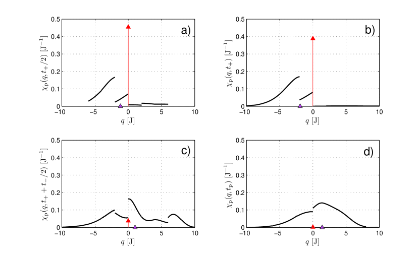
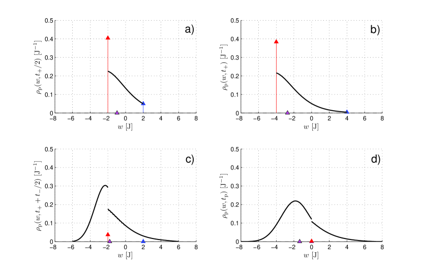
These two functions represent the main results of the present Section. They are illustrated in figures 2-4. We discuss their main features in section 5.

Figure 2: The probability density $\rho_{\mathrm{p}}(w,t)$ as a function of the work $w$ for the same parameters as in figure 1 (with positive $h_{1}$): a) $t=\frac{1}{2}t_{+}$ (middle of the first stroke), b) $t=t_{+}$ (end of the first stroke), c) $t=t_{+}+\frac{1}{2}t_{-}$ (middle of the second stroke), and d) $t=t_{+}+t_{-}$ (end of the limit cycle). The triangle on the work axis marks the mean work $W(t)$ at the corresponding times. The singular parts of $\rho_{\mathrm{p}}(w,t)$ are marked by arrows, where the arrow heights equal the weights of the corresponding delta functions [for example, in panel a), the left arrow height gives the probability that the system is initially in the second state and remains in it between the beginning of the cycle and the time $t=\frac{1}{2}t_{+}$; then the work done on the system equals $-\frac{1}{2}(h_{2}-h_{1})$].

Figure 3: The probability density $\chi_{\mathrm{p}}(q,t)$ as a function of the heat $q$ and for the same parameters as in figure 1 (with positive $h_{1}$): a) $t=\frac{1}{2}t_{+}$ (middle of the first stroke), b) $t=t_{+}$ (end of the first stroke), c) $t=t_{+}+\frac{1}{2}t_{-}$ (middle of the second stroke), and d) $t=t_{+}+t_{-}$ (end of the limit cycle). The triangles on the heat axis mark the mean heat $Q(t)$ at the corresponding times. The singular parts of $\chi_{\mathrm{p}}(q,t)$ are marked by the arrow, where the arrow height equals the weight of the corresponding delta function. For example, in a), the height of the arrow gives the probability that there was no transition between the states from the beginning of the cycle till the observation time $t=\frac{1}{2}t_{+}$. The heat exchanged in this case is zero.

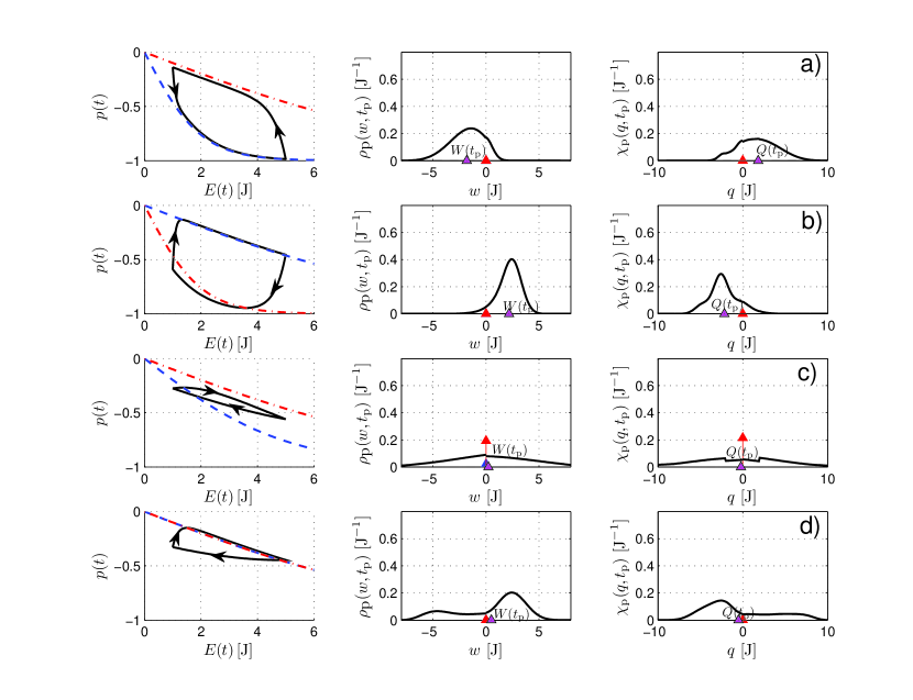
Figure 4: Probability densities $\rho_{\rm p}(w,t_{\mathrm{p}})$ and $\chi_{\rm p}(q,t_{\mathrm{p}})$ for the work and heat for four representative sets of the engine parameters. For every set we show also the limit cycle in the $p\!-\!\!E$ plane, where the corresponding equilibrium isotherms are marked by dashed (first stroke) and dot-dashed (second stroke) lines. In all cases we choose $h_{1}=1\;\mathrm{J}$, $h_{2}=5\;\mathrm{J}$, and $\nu=1\;\mathrm{s}^{-1}$. The remaining parameters are a) $t_{+}=50\;\mathrm{s}$, $t_{-}=10\;\mathrm{s}$, $\beta_{+}=0.5\;\mathrm{J}^{-1}$, $\beta_{-}=0.1\;\mathrm{J}^{-1}$ (bath of the first stroke is colder than of the second stroke), b) $t_{+}=50\;\mathrm{s}$, $t_{-}=10\;\mathrm{s}$, $\beta_{+}=0.1\;\mathrm{J}^{-1}$, $\beta_{-}=0.5\;\mathrm{J}^{-1}$ (exchange of $\beta_{+}$ and $\beta_{-}$ as compared to case a), leading to a change of the traversing of the cycle from counter-clockwise to clockwise and a sign reversal of the mean values $W(t_{\mathrm{p}})\equiv\langle\,\mathsf{W}(t_{\mathrm{p}})\,\rangle$ and $Q(t_{\mathrm{p}})\equiv\langle\,\mathsf{Q}(t_{\mathrm{p}})\,\rangle$), c) $t_{+}=2\;\mathrm{s}$, $t_{-}=2\;\mathrm{s}$, $\beta_{+}=0.2\;\mathrm{J}^{-1}$, $\beta_{-}=0.1\;\mathrm{J}^{-1}$ (a strongly irreversible cycle traversed clockwise with positive work), d) $t_{+}=20\;\mathrm{s}$, $t_{-}=1\;\mathrm{s}$, $\beta_{\pm}=0.1\;\mathrm{J}^{-1}$ (no change in temperatures, but large difference in duration of the two strokes; $W(t_{\mathrm{p}})$ is necessarily positive).

4 Engine performance

As shown in section 2, the occupation probabilities during the limit cycle are $\mathbb{R}_{{\rm p}}(t)\,\left|p^{{\rm stat}}\right\rangle$ with $\mathbb{R}_{{\rm p}}(t)$ given by equation (25). These probabilities are ensemble averaged quantities and cannot describe fluctuations of the engine’s performance. But they render the energetics in terms of mean values as we discuss now.

During the limit cycle, the internal energy $U(t)=\sum_{i=1}^{2}E_{i}(t)p_{i}(t)$ changes as

$$\frac{\mathrm{d}}{\mathrm{d}t}U(t)=\sum_{i=1}^{2}E_{i}(t)\frac{\mathrm{d}}{\mathrm{d}t}p_{i}(t)+\sum_{i=1}^{2}p_{i}(t)\frac{\mathrm{d}}{\mathrm{d}t}E_{i}(t)=\frac{\mathrm{d}}{\mathrm{d}t}\left[Q(t)+W(t)\right],\quad\,\,\,t\in[0,t_{{\rm p}}]\,.$$ (71)

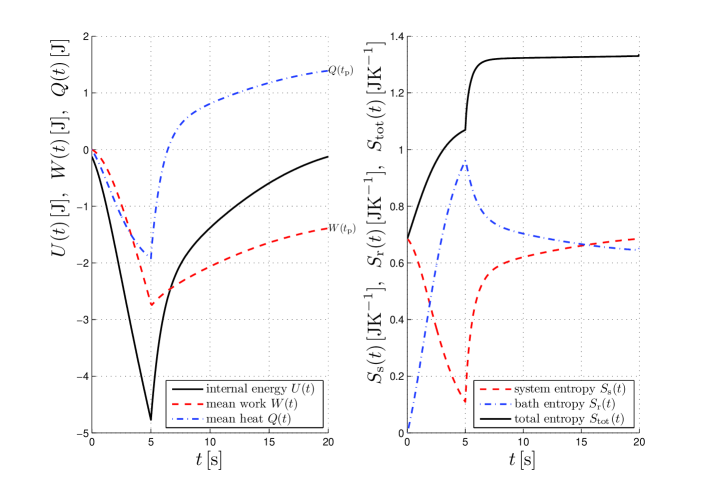
Here $Q(t)\equiv\langle\,\mathsf{Q}(t)\,\rangle$ is the mean heat received from the reservoirs during the period between the beginning of the limit cycle and the time $t$. Analogously $W(t)\equiv\langle\,\mathsf{W}(t)\,\rangle$ is the mean work done on the system from the beginning of the limit cycle till the time $t$. If $W(t)<0$, the positive work $-W(t)$ is done by the system on the environment. Therefore the oriented areas enclosed by the limit cycle in figure 1 and in figure 4 represent the work $W_{\mathrm{out}}\equiv-W(t_{\mathrm{p}})$ done by the engine on the environment per cycle. These areas approach maximal absolute values in the quasi-static limit. The internal energy, being a state function, fulfills $U(t_{{\rm p}})=U(0)$. Therefore, if the work $W_{\mathrm{out}}$ is positive, the same total amount of heat has been transferred from the two reservoirs during the cycle. The case $W_{\mathrm{out}}>0$ cannot occur if both reservoirs would have the same temperature. That the perpetuum mobile is actually forbidden can be traced back to the detailed balance condition in (1).

Figure 5: Thermodynamic quantities as functions of time during the limit cycle for the same set of parameters as in the upper panel of figure 1 (positive $h_{1}$). Left panel: internal energy, mean work done on the system, and mean heat received from both reservoirs; the final position of the mean work curve marks the work done on the system per cycle $W(t_{\rm p})$. Since $W(t_{\rm p})<0$, the work $W_{\rm out}=-W(t_{\rm p})$ has been done on the environment. The internal energy returns to its original value and, after completion of the cycle, the absorbed heat $Q(t_{\rm p})$ equals the negative work $-W(t_{\rm p})$. Right panel: entropy $S_{\mathrm{s}}(t)$ of the system and $S_{\mathrm{r}}(t)$ of the bath, and their sum $S_{\rm tot}(t)$; after completing the cycle, the system entropy re-assumes its initial value. The difference $S_{\rm tot}(t_{\rm p})-S_{\rm tot}(0)>0$ equals the entropy production per cycle. It is always positive and quantifies the degree of irreversibility of the cycle.

We denote the system entropy at time $t$ as $S_{\mathrm{s}}(t)$, and the reservoir entropy at time $t$ as $S_{\mathrm{r}}(t)$. They are given by

$$\frac{S_{\mathrm{s}}(t)}{k_{\mathrm{B}}}=-\left[p_{1}(t)\ln p_{1}(t)+_{2}(t)\ln p_{2}(t)\right],$$ (72)

$$\frac{S_{\mathrm{r}}(t)}{k_{\mathrm{B}}}=-\beta_{+}\int_{0}^{t_{+}}\mathrm{d}t^{\prime}E_{1}(t^{\prime})\frac{\mathrm{d}}{\mathrm{d}t^{\prime}}[p_{1}(t^{\prime})-p_{2}(t^{\prime})]-\beta_{-}\int_{t_{+}}^{t_{{\rm p}}}\mathrm{d}t^{\prime}E_{1}(t^{\prime})\frac{\mathrm{d}}{\mathrm{d}t^{\prime}}[p_{1}(t^{\prime})-p_{2}(t^{\prime})].$$ (73)

Upon completing the cycle, the system entropy re-assumes its value at the beginning of the cycle. On the other hand, the reservoir entropy is controlled by the heat exchange. Owing to the inherent irreversibility of the cycle we observe always a positive entropy production per cycle, $S_{\mathrm{r}}(t_{{\rm p}})-S_{\mathrm{r}}(0)>0$. The total entropy $S_{\mathrm{tot}}(t)=S_{\mathrm{s}}(t)+S_{\mathrm{r}}(t)$ increases for any $t\in[0,t_{{\rm p}}]$. The rate of the increase is the larger the stronger is the representative point in the $p\!-\!\!E$ diagram deviates from the corresponding equilibrium isotherm (a strong deviation, e.g., can be seen in the $p\!-\!\!E$ diagram in figure 4c). Due to the instantaneous exchange of the baths at times $t_{+}$ and $t_{+}+t_{-}$ in the model considered here, a strong increase of $S_{\mathrm{tot}}(t)$ always occurs after these time instants. A representative example of the overall behavior of the thermodynamic quantities (mean work and heat, and entropies) during the limit cycle is shown in figure 5.

An important characteristics of the engine is its power output $P_{\mathrm{out}}$ and its efficiency $\mu$. They are defined as

$$P_{\mathrm{out}}\equiv\frac{W_{\mathrm{out}}}{t_{\mathrm{p}}}\,\,\,,\,\,\,\mu\equiv\frac{W_{\mathrm{out}}}{Q_{\mathrm{in}}}\,\,,$$ (74)

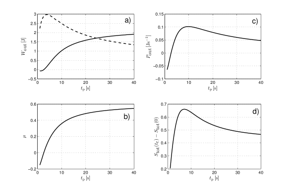
where $Q_{\mathrm{in}}$ is the total heat absorbed by the system per cycle. The performance of the engine characterized by the output work, efficiency, output power, and entropies from equations (72) and (73) are shown in figure 6 and figure 7.

In figure 6 the performance is displayed as a function of the cycle duration $t_{\rm p}$ for $t_{+}=t_{-}=t_{\mathrm{p}}/2$. With increasing $t_{\rm p}$, the output work and the efficiency increase whereas the output power and the entropy production first increase up to a maximum and thereafter they decrease when approaching the quasi-static limit ($t_{{\rm p}}\rightarrow\infty$). Notice that the maximum efficiency and output power occur at different values of $t_{\rm p}$. In figure 6a) we show also the standard deviation of the output work, which was calculated from the work probability density $\rho_{{\mathrm{p}}}(w,t_{\mathrm{p}})$. Finally, let us note that the values $\beta_{+}=0.5$ $\mathrm{J}^{-1}$ and $\beta_{-}=0.1$ $\mathrm{J}^{-1}$ used in figure 6 give the Carnot efficiency $\mu_{\mathrm{C}}=0.8$. This should be compared with the efficiency of the engine for a long period $t_{\rm p}$, that is, with the value $\mu\approx 0.6$. As discussed above, the Carnot efficiency cannot be reached here even for $t_{{\rm p}}\rightarrow\infty$, due to the immediate temperature changes at times $t_{+}$ and $t_{+}+t_{-}$.

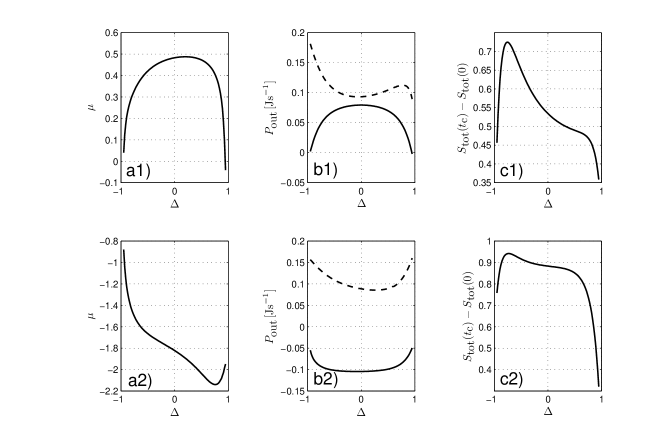
In figure 7 we have fixed $t_{{\rm p}}$ and plotted the behavior as function of the time asymmetry (or time splitting) parameter $\Delta=(t_{+}-t_{-})/t_{{\rm p}}$. As can be seen from the upper three panels in figure 7, there exist also a maximal efficiency and a maximal output power with respect to a variation of the time asymmetry parameter (as long as the engine performs work, i.e., $W_{\mathrm{out}}>0$). Again, the optimal parameter $\Delta$, where these maxima occur, is different for the efficiency and output power. In a reversed situation, considered in the lower three panels in figure 7, where the work is performed on the engine ($W_{\mathrm{out}}<0$), minima of the efficiency and output power occur.

Figure 6: The engine performance versus the duration of the limit cycle $t_{\pm}$ for $t_{+}=t_{-}={\textstyle\frac{1}{2}}t_{\rm p}$ and otherwise the same parameters as in the upper part of figure 1 (positive $h_{1}$). Both the output work $W_{\mathrm{out}}$ in a) and the efficiency $\mu$ in b) increase with $t_{{\rm p}}$. The output power $P_{\mathrm{out}}$ in c) assumes a maximum at a special cycle duration. The dashed line in a) marks the standard deviation of the output work, calculated from the work density $\rho_{\rm p}(w,t_{\mathrm{p}})$. Notice that the work fluctuation is comparatively high close to the cycle duration, where the maximal output power is found. In the long-period limit $t_{{\rm p}}\rightarrow\infty$, the cycle still represents a non-equilibrium process (due to the construction of the model, see text), and hence the entropy production $S_{\rm tot}(t_{\rm p})-S_{\rm tot}(0)$ in d) remains positive, approaching a specific asymptotic value.

Figure 7: The engine performance characterized by the efficiency $\mu$, output power $P_{\mathrm{out}}$, and entropy production $S_{\mathrm{tot}}(t_{{\rm p}})-S_{\mathrm{tot}}(0)$, as a function of the asymmetry parameter $\Delta=(t_{+}-t_{-})/t_{{\rm p}}$ for a fixed period $t_{\rm p}=20\;\mathrm{s}$ and the same parameters $h_{1}=1\;\mathrm{J}$, $h_{2}=5\;\mathrm{J}$, $\nu=1\;\mathrm{s}^{-1}$ as in the upper panel of figure 1. In a1)–c1) the bath during the first stroke is colder than during the second stroke: $\beta_{+}=0.5\;\mathrm{J}^{-1}$ and $\beta_{-}=0.1\;\mathrm{J}^{-1}$. Notice that the value $\Delta$ of maximum efficiency does not correspond to that of maximum output power. In a2)-c2) the reciprocal bath temperatures are interchanged compared to cases a1)-c1), $\beta_{+}=0.1\;\mathrm{J}^{-1}$ and $\beta_{-}=0.5\;\mathrm{J}^{-1}$. The dashed curves in b1) and b2) show the standard deviation of the output power calculated from $\rho_{\rm p}(w,t_{\mathrm{p}})$.

5 Discussion

The overall properties of the engine critically depend on the two dimensionless parameters $a_{\pm}=\nu/(2\beta_{\pm}|v_{\pm}|)$. We call them reversibility parameters. For a given branch, say the first one, the parameter $a_{+}$ represents the ratio of two characteristic time scales. The first one, $1/\nu$, is given by the attempt rate of the internal transitions [29]. The second scale is proportional to the reciprocal driving velocity. Contrary to the first scale, the second one is fully under the external control. Moreover, the reversibility parameter is proportional to the absolute temperature of the heat bath.

Let us first consider the work probability density (69) within the first stroke in the case $h_{2}>h_{1}$, c.f. figure. 2a). In essence, $\rho_{\rm p}(w,t)$ is given by a linear combination of the functions equations (60)-(63). It vanishes outside the common support $[\,-v_{+}t,v_{+}t\,]$ which broadens linearly in time. Besides the continuous part located within the support, the diagonal elements $g_{ii}(w,0,t,0)$ display a singular part represented by delta functions at the borders of the support. The delta functions correspond to the paths with no transitions between the states. Specifically, the weight of the delta function located at $w=v_{+}t$ represents the probability that the system starts in the first state and remains there up to time $t$. The weight corresponding to the first level decreases with increasing time and vanishes for $t\rightarrow\infty$. On the contrary, the weight of the delta function at $-v_{+}t$ approaches the nonzero limit $2\beta_{+}/(1+c_{+})^{a_{+}}$ for $t\rightarrow\infty$, which is the probability that the a path starts in the second state and never leaves it.

Within the second stroke, the density $\rho_{\rm p}(w,t)$ results from the integral of the propagators for the individual strokes, c.f. equation (66). Due to the integration, the singular parts of the cycle propagator $\mathbb{G}_{+}(w,0;t)$ are now situated inside the support, at the values $w=-v_{+}t_{+}+|v_{-}|(t-t_{+})$ and $w=v_{+}t_{+}-|v_{-}|(t-t_{+})$. The two delta functions approach each other and, upon completing the cycle, they coincide at the point $w=0$. The nonsingular component of the density is no more continuous [30]. The jumps are located at the positions of the delta functions and their magnitudes correspond to the weights of the delta functions (for a discussion of the origin of these jumps, see [31]).

If both reversibility parameters $a_{\pm}$ are small, the isothermal processes during both branches strongly differs from the equilibrium ones. The signature of this case is a flat continuous component of the density $\rho_{\rm p}(w,t)$ and a well pronounced singular part. The strongly irreversible dynamics occurs if one or more of the following conditions hold. First, if $\nu$ is small, the transitions are rare and the occupation probabilities of the individual energy levels are effectively frozen during long periods of time. Therefore they lag behind the Boltzmann distribution which would correspond to the instantaneous positions of the energy levels. More precisely, the population of the ascending (descending) energy level is larger (smaller) than it would be during the corresponding reversible process. As a result, the mean work done on the system is necessarily larger than the equilibrium work. Secondly, a similar situation occurs for large driving velocities $v_{\pm}$. Due to the rapid motion of the energy levels, the occupation probabilities again lag behind the equilibrium ones. Thirdly, the strong irreversibility occurs also in the low temperature limit. In the limit $a_{\pm}\rightarrow 0$, the continuous part vanishes and $\rho_{\rm p}(w,t_{\rm p})=\delta(w)$.

In the opposite case of large reversibility parameters $a_{\pm}$, both branches in the $p\!-\!\!E$ plane are located close to the reversible isotherms. The singular part of the density $\rho_{\rm p}(w,t)$ is suppressed and the continuous part exhibits a well pronounced peak. From general considerations [11], the density must approach a Gaussian shape. Our results allow a detailed study of this approach. Let us denote as $F(\beta,E)$ the free energy of a two level system with energies $\pm E$ at temperature $T=1/(k_{{\rm B}}\beta$, i.e., $F(\beta,E)=-\frac{1}{\beta}\ln[2\cosh(\beta E)]$. Let us further define

$$W_{\mathrm{rev}}(t)=\left\{\begin{array}[]{ll}F(\beta_{+},E_{1}(t))-F(\beta_{+},E_{1}(0)),&t\in[0,t_{+}],\\ F(\beta_{-},E_{1}(t))-F(\beta_{-},E_{1}(t_{+}))+F(\beta_{+},E_{1}(t_{+}))-F(\beta_{+},E_{1}(0)),&t\in[t_{+},t_{{\rm p}}].\end{array}\right.$$

(76)

This is simply the reversible work done on the system if we transform its state from the initial equilibrium state (with the energies fixed at $\pm E_{1}(0)$) to another equilibrium state (with the energies fixed at the values $\pm E_{1}(t)$). For large reversibility parameters $a_{\pm}$, the peak of the work density $\rho_{\rm p}(w,t_{\rm p})$ occurs in the vicinity of the value $W_{\mathrm{rev}}(t)$ and with increasing $a_{\pm}$, the peak collapses to a delta function,

$$\lim_{a_{\pm}\rightarrow\infty}\rho_{\rm p}(w,t)=\delta(w-W_{\mathrm{rev}}(t))\,\,.$$ (77)

The main features of the heat probability density $\chi_{\mathrm{p}}(q,t)$ from equation (70) are, as we have seen in section 3, closely related to the work through simple shifts of the independent variable $q$. However, there are some interesting differences. While the work is conditioned by the external driving, the heat exchange occurs as a consequence of the transitions between the system states. The instantaneous positions of the energies at the instant of the transition give the magnitude of the heat exchange related with the given transition. From this perspective, if there are no transitions, the exchanged heat is zero. As a consequence, the singular part of the probability density $\chi_{\mathrm{p}}(q,t)$ is always situated at $q=0$ and the weight of the delta function at origin equals the sum of the weights of the delta functions in the work density $\rho_{\rm p}(w,t)$. The support of the heat density is given by the largest possible value of the level splitting during the limit cycle. Within the first stroke the support broadens linearly with time as $[-2h_{1}-2v_{+}t,2h_{1}+2v_{+}t]$, up to its maximum width $[-2h_{2},2h_{2}]$ at the end of the stroke. Within the second stroke the energy difference decreases and the support remains unchanged. The non-singular part of the heat density always displays discontinuities inside the support, even during the first stroke. In contrast to $\langle\,i\,|\,{\mathbb{G}}_{\rm p}(w,t)|\,j\,\rangle$, the individual elements $\langle\,i\,|\,{\mathbb{K}}_{\rm p}(q,t)|\,j\,\rangle$ in equation (70) have different supports.

In the the strongly reversible regime each element $\langle\,i\,|\,{\mathbb{G}}_{\rm p}(w,t)|\,j\,\rangle$ exhibits a Gaussian shape situated at $W_{\mathrm{rev}}(t)$. The shift transformation maps the Gaussian function onto four different positions depending on the specific matrix element $\langle\,i\,|\,{\mathbb{K}}_{\rm p}(q,t)|\,j\,\rangle$ in question. In the reversible limit we have

$$\lim_{a_{\pm}\rightarrow\infty}\langle\,i\,|\,{\mathbb{K}}_{\rm p}(q,t)|\,j\,\rangle=\delta\left(\,q-u_{ij}(t)+W_{\mathrm{rev}}(t)\,\right)\,\,.$$ (78)

Using this form in equation (70) and calculating the mean accepted heat, we get $Q(t)=U(t)-U(0)-W_{\mathrm{rev}}(t)$. In the opposite limit, if $a_{\pm}\rightarrow 0$, we have $\chi_{\mathrm{p}}(q,t)\rightarrow\delta(q)$ for any $t$.

According to the second law of thermodynamics, the mean work $W(t)=\langle\,\mathsf{W}(t)\,\rangle$ must fulfill $|W(t)|\geq|W_{\rm rev}(t)|$. On the other hand, there always exists a fraction of the paths which, individually, display the inequality $|\widetilde{w}({\rm path},t)|<|W_{\rm rev}(t)|$, where $\widetilde{w}({\rm path},t)$ denotes the work done on the system if it evolves along the indicated path. Using the exact work probability density, we can calculate the total weight of these trajectories. Specifically, in the case $W_{\rm rev}(t)>0$,

$$\mathop{\mathrm{Prob}}\,\left\{\,\textsf{W}(t)<W_{\rm rev}(t)\,\right\}=\int_{-\infty}^{W_{\rm rev}(t)}\,\mathrm{d}w\,\rho_{\rm p}(w,t)\,\,.$$ (79)

If $W_{\rm rev}(t)<0$, we would have to integrate over the interval $(W_{\rm rev}(t),\infty,)$.

Let us finally note that in view of the rather complex structure of the work and heat probability densities, we performed several independent tests. First of all, the densities $\rho_{\rm p}(w,t)$ and $\chi_{\mathrm{p}}(q,t)$ must be nonnegative functions fulfilling the normalization conditions, e.g. $\int_{-\infty}^{\infty}\,\mathrm{d}w\,\rho_{\rm p}(w,t)=1$ for any $t\in[0,t_{\mathrm{p}}]$. Secondly, we have two different procedures to calculate the first moment $W(t)=\langle\,\mathsf{W}(t)\,\rangle$. One can either start with the density $\rho_{\rm p}(w,t)$ and evaluate the required $w$-integral, or one directly employs the solution of the rate equation as in Sec. IV. Another inspection is based on the Jarzynski identity [7, 8]. In our setting, consider the case $\beta_{\pm}=\beta$. After completing the cycle, the system returns to the original state. Therefore we have $W_{\mathrm{rev}}(t_{\rm p})=F(\beta,E_{1}(t_{\rm p}))-F(\beta,E_{1}(0))=0$ and the Jarzynski identity reduces to $\langle\,\exp\left[-\beta\mathsf{W}(t_{\rm p})\right]\,\rangle=1$. Using the explicit form of the work probability density we have verified that the integral $\int_{-\infty}^{\infty}\,\mathrm{d}w\,\exp(-\beta w)\rho_{\rm p}(w,t_{\rm p})$ actually equals one. Finally, we have studied the probability densities $\rho_{\rm p}(w,t)$, $\chi_{\mathrm{p}}(q,t)$ by computer simulation. In fact, we have developed two exact simulation methods. Each of them uses a specific algorithm to generate paths of the time-non-homogeneous Markov process $\mathsf{D}(t)$. Parts of these simulation results have been published in [31] and confirm the analytical results.

6 Conclusions

We have investigated a simple example of a microscopic heat engine, which is exactly solvable. Based on mean thermodynamic quantities, the engine performance is characterized by the occupation probabilities of the energy levels following from the master equation. The more challenging exact calculation of the work and heat probability densities allowed us to study the fluctuation properties in detail. A notable result is that the engine can be tuned to maximize its output power, but the fluctuations of this quantity in the corresponding optimal regime of control parameters are comparatively high.

The present setting can be expanded in various directions. One can address various problems concerning the thermodynamic optimization. Another option would be the embodiment of additional (e.g., adiabatic) branches. The role of the working medium can be assigned to other systems that exhibit more complicated dynamics (e.g., diffusing particles in the presence of time-dependent forces, or, variants of the generalized master equation). It would be also interesting to investigate settings with a nonlinear driving of the energy levels. A nontrivial generalization would be the inclusion of a third energy level. Having the three levels one can couple the system (different pairs of forth-back transitions between the levels) simultaneously to reservoirs at different temperatures, so that the system approaches a non-equilibrium steady state without driving [32]. Including a driving and forming an operational cycle, there is no serious obstacle in repeating the present analysis for this system, which has some additional intriguing properties compared to the two-level system considered here (as, e.g., negative specific heats).

Another possibility is an incorporation of specific forms of transition rates [33] that describe the stretching of biomolecules in some realistic manner. In such problem, the histogram of the work is experimentally accessible [33]. Particularly, in the experiments one can also determine the probability of having certain number of transitions between the folded and the unfolded conformation of the biomolecule during its mechanical stretching [33]. In our formulation, this information is encoded in the counting statistics of the underlying random point process [34] and can be extracted from the perturbation expansion of the propagators which solve our dynamical equations. Calculations in this direction are in progress and will be reported elsewhere.

References

• [1] Evans D J and Searles D J, 2002 Adv. Chem. Phys. 51 1529
• [2] Ritort F, 2008 Adv. Chem. Phys. 137 31
• [3] Seifert U, 2008 Eur. Phys. J. B 64 423
• [4] Bochkov G N and Kuzovlev Y E  1981 Physica A 106 443; ibid. 1981 Physica A 106 480
• [5] Evans D J, Cohen E G D and Morriss G P, 1993 Phys. Rev. Lett. 71 2401
• [6] Gallavotti G and Cohen E G D, 1995 Phys. Rev. Lett. 74 2401
• [7] Jarzynski C, 1997 Phys. Rev. Lett. 78 2690; ibid. 1997 Phys. Rev. E 56 5018
• [8] Crooks G E, 1998 J. Stat. Phys. 90 1481; ibid. 1999 Phys. Rev. E 60 2721; ibid. 2000 Phys. Rev. E 61 2361
• [9] Maes C, 2003 Sém. Poincaré 2 29
• [10] Hatano T and Sasa S, 2001 Phys. Rev. Lett. 86 3463
• [11] Speck T and Seifert U, 2004 Phys. Rev. E 70, 066112
• [12] Seifert U, 2005 Phys. Rev. Lett. 95 040602
• [13] Schuler S, Speck T, Tietz C, Wachtrup J, Seifert U, 2005 Phys. Rev. Lett. 94 180602
• [14] Esposito M and Mukamel S, 2006 Phys. Rev. E 73 046129
• [15] Sekimoto K, Takagi F, and Hondou T, 2000 Phys. Rev. E 62 7759
• [16] van den Broeck C, Kawai R and Meurs P, 2004 Phys. Rev. Lett. 93 090601
• [17] Schmiedl T and Seifert U, 2008 Europhys. Lett. 81 20003
• [18] Henrich M J, Rempp F and Mahler G, 2007 Eur. Phys. J. Special Topics 151 157
• [19] Allahverdyan A E, Johal R S J and Mahler G, 2008 Phys. Rev. E 77 041118
• [20] Curzon F L and Ahlborn B, 1975 Am. J. Phys. 43 22
• [21] Subrt E, Chvosta P, 2007 J. Stat. Mech. P09019
• [22] Gammaitoni L, Häggi P, Jung P and Marchesoni F, 1998 Rev. Mod. Phys. 70 223
• [23] Slater L J, 1960 Confluent Hypergeometric Functions (New York: Cambridge University Press)
• [24] Talkner P, Burada P S and Hänggi P, 2008 Phys. Rev. E 78 011115
• [25] Jarzynski C, 2006 Phys. Rev. E 73 046105
• [26] Hatano T, 1999 Phys. Rev. E 60 R5017
• [27] Imparato A and Peliti L, 2005 Europhys. Lett. 69 643
• [28] Imparato A and Peliti L, 2005 Europhys. Lett. 70 740; ibid. 2005 Phys. Rev. E 72 046114
• [29] Note that due to the choice of the Glauber rates in equation (3), the relaxation rate [λ1(t)+λ2(t)]delimited-[]subscript𝜆1𝑡subscript𝜆2𝑡[\lambda_{1}(t)+\lambda_{2}(t)] (for frozen energy levels at any time instant t𝑡t) is bounded by 2ν2𝜈2\nu.
• [30] Only delta-functions are referred to as singularities here.
• [31] Einax M and Maass P, 2009 Phys. Rev. E 80 020102(R)
• [32] Zia R K P, Praestgaard E L and Mouritsen O G, 2002 Am. J. Phys. 70 384
• [33] Manosas M, Mossa A, Forns N, Huguet J M and Ritort F , 2009 J. Stat. Mech. P02061
• [34] Slater L J, 1960 Random Point Processes (New York: Wiley)