Solving the Poisson equation on small aspect ratio domains using unstructured meshes

Abstract

We discuss the ill conditioning of the matrix for the discretised Poisson equation in the small aspect ratio limit, and motivate this problem in the context of nonhydrostatic ocean modelling. Efficient iterative solvers for the Poisson equation in small aspect ratio domains are crucial for the successful development of nonhydrostatic ocean models on unstructured meshes. We introduce a new multigrid preconditioner for the Poisson problem which can be used with finite element discretisations on general unstructured meshes; this preconditioner is motivated by the fact that the Poisson problem has a condition number which is independent of aspect ratio when Dirichlet boundary conditions are imposed on the top surface of the domain. This leads to the first level in an algebraic multigrid solver (which can be extended by further conventional algebraic multigrid stages), and an additive smoother. We illustrate the method with numerical tests on unstructured meshes, which show that the preconditioner makes a dramatic improvement on a more standard multigrid preconditioner approach, and also show that the additive smoother produces better results than standard SOR smoothing. This new solver method makes it feasible to run nonhydrostatic unstructured mesh ocean models in small aspect ratio domains.

1 Introduction

There are many processes in the ocean (such as separating Western boundary currents, and density overflows) which are small in scale and restricted to particular regions, but which form crucial components of the global ocean circulation mechanism. It therefore seems attractive to design ocean models which use the finite element method on fully unstructured meshes in order to incorporate some of these smaller scale features into a global ocean model (see Pain et al. (2005) for background and references). However, there are numerous pitfalls to negotiate in order to achieve this goal, arising from the fact that the global ocean is very thin: the horizontal lengthscale is thousands of times larger than the vertical lengthscale.

One particular issue arises if one wishes to relax the hydrostatic approximation (Pedlosky, 1987), allowing for a model which is valid on both small and large scales. The nonhydrostatic pressure is obtained by solving a three dimensional elliptic problem with very large eigenvalues resulting from the horizontal scales, as well as very small eigenvalues resulting from the vertical scales. This means that the system is very ill conditioned. Since the Conjugate Gradient method, which is typically used for finite element discretisations with many degrees of freedom, has a convergence rate which scales with the square root of the condition number (see Shewchuk (1994) for example), this can have a catastrophic effect on the performance of the numerical model.

In the ocean modelling context this problem was first encountered by Marshall et al. (1997). A solution strategy was proposed using a vertical preconditioner which solves the vertically integrated (aspect ratio independent) equations and then distributes the solution throughout the mesh. It was shown that the use of this preconditioner resulted in nonhydrostatic simulations which were as fast as hydrostatic simulations at the same resolution. This strategy, has since been used in a number of nonhydrostatic ocean models, including those on horizontally unstructured grids such as Fringer et al. (2006). However, the vertical averaging depends on the computational mesh being organised in vertical layers. This prohibits more general types of vertically unstructured meshes which may be required for multiscale simulations in which a small scale process is resolved within a large scale flow, or for hybrid meshes which accommodate both terrain following and isopycnal (constant density) layers.

In this paper we extend the vertical averaging strategy so that it can be applied to vertically unstructured meshes of large-scale ocean modelling such as those that can be used in the Imperial College Ocean Model (ICOM) (Piggott et al., 2008). The extension is formulated by using the vertical extrapolation operator, which takes any point in the domain and returns the value of a function at the top surface directly above that point. This operator is the dual of the vertical integration operator, and can easily be approximated on a vertically unstructured mesh. This extension is described within the context of the algebraic multigrid method; the framework also shows how to incorporate further algebraic multigrid stages into the “smoother”, which reconstructs the solution of the vertically integrated equations throughout the domain. This turns out to be necessary when a genuinely multiscale mesh is used in which the aspect ratio becomes $\mathcal{O}(1)$ at the smallest scales. The aim is to obtain a numerical solver which has a convergence rate which is independent of the aspect ratio.

The rest of this paper is organised as follows. In section 2, we describe the type of problems we wish to solve on small aspect ratio domains, and motivate them using the ocean modelling applications. In particular, this section explains why we cannot avoid solving an elliptic problem with Neumann boundary conditions on all surfaces, which is precisely the problem which gives rise to ill-conditioning. In section 3 we formulate the problem as a finite element approximation, in order to fix notation, and in section 4 we compute some estimates on the condition number for the Neumann boundary condition case, as well as the case where Dirichlet boundary conditions are imposed on the top surface. It is observed that imposing the Dirichlet boundary conditions removes the small eigenvalues, and this motivates a preconditioning strategy in which one first eliminates the interior degrees of freedom to obtain an equation for the solution on the top surface, then one uses this surface solution as a Dirichlet boundary condition to reconstruct the solution throughout the domain. This paves the way for section 5 in which our proposed preconditioner is introduced, in the context of algebraic multigrid preconditioners for the Conjugate Gradient method. The preconditioner is tested in various examples in section 6. Finally, in section 7 we give a summary and outlook.

2 Background: oceanographic applications

In this section we describe how the pressure Poisson equation arises in nonhydrostatic models, which motivates the need to develop efficient solvers for this equation in small aspect ratio domains. We shall also explain the types of boundary conditions that are imposed, in particular we shall explain why we need to tackle the problem of solving the pressure Poisson equation with Neumann boundary conditions.

2.1 Nonhydrostatic equations

The nonhydrostatic Euler-Boussinesq equations for a rotating stratified fluid on an $f$-plane are

$$\rho_{0}\left(\frac{\partial\boldsymbol{u}}{\partial t}+\boldsymbol{u}\cdot\nabla\boldsymbol{u}+f\hat{\boldsymbol{z}}\times\boldsymbol{u}\right) = -\nabla p-g\rho\hat{\boldsymbol{z}},$$ (1)

$$\nabla\cdot\boldsymbol{u} = 0,$$ (2)

$$\frac{\partial T}{\partial t}+\boldsymbol{u}\cdot\nabla T = 0,$$ (3)

where $\boldsymbol{u}$ is the velocity, $\rho_{0}$ is the (constant) reference density, $\hat{\boldsymbol{z}}$ is the unit vector in the upward direction, $f$ is the Coriolis parameter, $p$ is the pressure, $g$ is the gravitation constant, $T$ is the potential temperature and $\rho$ is a prescribed function of the temperature. Here we do not complicate the exposition by including viscosity or diffusivity terms, or dependence of the density on salinity or pressure.

We solve the problem in an “ocean shaped” domain $\Omega$ with bottom boundary $\partial\Omega_{\operatorname{\text{floor}}}$, coastal boundaries $\partial\Omega_{\operatorname{\text{coast}}}$ and top boundary $\partial\Omega_{\operatorname{\text{top}}}$ (which may be allowed to move up and down to accommodate surface waves). The horizontal extent of the domain is $L$, and the vertical extent of the domain is $H$; in this paper we concentrate on the difficulties when the aspect ratio $H/L$ of the domain is very small ($H/L\approx 1/1000$ for an ocean basin). We shall parameterise the top surface by

$$z=\eta(x,y),$$

with $\eta=0$ when the fluid is at rest, and make the additional simplifying assumption that the coastal boundaries are vertical.

We consider two types of boundary conditions:

• Rigid lid:

  $$\boldsymbol{u}\cdot\boldsymbol{n} = 0,\quad\boldsymbol{x}\in\partial\Omega_{\operatorname{\text{floor}}}\cup\partial\Omega_{\operatorname{\text{coast}}}\cup\partial\Omega_{\operatorname{\text{top}}},$$

  $$\eta = 0,$$

  for a constant top surface height $z=0$.

• Free surface:

  $$\boldsymbol{u}\cdot\boldsymbol{n} = 0,\quad\boldsymbol{x}\in\partial\Omega_{\operatorname{\text{floor}}}\cup\partial\Omega_{\operatorname{\text{coast}}},$$

  $$p = p_{a},\quad\boldsymbol{x}\in\partial\Omega_{\operatorname{\text{top}}},$$

  $$\eta_{t} = -\boldsymbol{u}_{H}\cdot\nabla_{H}\eta-w=-\frac{\boldsymbol{u}\cdot\boldsymbol{n}}{\boldsymbol{n}\cdot\hat{\boldsymbol{z}}}.$$ (4)

In the subsequent section we shall show that both of these equations effectively result in an ill conditioned pressure equation in the small aspect ratio limit; this always occurs for the rigid lid case and also occurs for the free surface case when one wishes to take large timesteps and has an unstructured mesh.

2.2 Solving for the pressure

The role of the pressure in these equations is as a Lagrange multiplier which enforces the incompressibility condition (2) (in fact it enforces that the solution to $D_{t}+\nabla\cdot(D\boldsymbol{u})=0$ is $D=1$, and equation (2) is then a direct consequence, see Holm et al. (1998)) for example. To solve for the pressure, take the divergence of equation (1):

$$-\nabla^{2}p=\nabla\cdot\left(\rho_{0}\left(\boldsymbol{u}\cdot\nabla+f\hat{\boldsymbol{z}}\times\right)\boldsymbol{u}+\hat{\boldsymbol{z}}g\rho\right),$$

which is a Poisson equation for the pressure $p$, given the other variables $\boldsymbol{u}$ and $T$. In practise, one usually solves for the pressure update $\rho_{0}\phi/\Delta t=p^{n+1}-p^{n}$ (where $p^{n}$ is the pressure at time level $n$) using one of the families of projection methods based on Chorin (1967); Temam (1969). These methods are typically predictor-corrector schemes in which a predictor $\boldsymbol{u}^{*}$ is obtained using the pressure from the previous timestep, without enforcing the incompressibility condition (2), and then constructing a correction

$$\boldsymbol{u}^{n+1}=\boldsymbol{u}^{*}-\nabla\phi,$$ (5)

subject to

$$\nabla\cdot\boldsymbol{u}^{n+1}=0.$$

Taking the divergence of equation (5) gives

$$-\nabla^{2}\phi=-\nabla\cdot\boldsymbol{u}^{*}.$$ (6)

For more details, see Karniadakis and Sherwin (2005); Gresho and Sani (2000).

On slip boundaries where $\boldsymbol{u}\cdot\boldsymbol{n}=0$, since $\boldsymbol{u}^{*}$ already satisfies the boundary conditions, then

$$\frac{\partial\phi}{\partial n}=0,$$ (7)

so that $\boldsymbol{u}^{n+1}$ keeps the same boundary conditions. In the free surface case, the pressure must stay constant on the surface, so $\phi$ satisfies the zero Dirichlet condition on the top surface:

$$\frac{\partial\phi}{\partial n}=0\text{ on }\partial\Omega_{\operatorname{\text{coast}}}\cup\partial\Omega_{\operatorname{\text{floor}}},\quad\phi=0\text{ on }\partial\Omega_{\operatorname{\text{top}}}.$$

However, the equations support free surface (barotropic) waves which are very fast compared to the other dynamics. Moreover, the highest frequency waves have small amplitudes and we are not concerned with the details of their evolution in large scale models. The standard ocean modelling approach is to apply a splitting method in which one integrates the barotropic waves in time using a much smaller timestep; the remaining (baroclinic) dynamics is then integrated using a larger timestep (see Shchepetkin and McWilliams (2005) for example). However, if the mesh used is unstructured in the vertical direction (i.e. the mesh is not arranged into layers) then it is not possible to obtain such a splitting. An alternative approach which is often used in coastal engineering applications (see Labeur and Pietrzak (2005) for example), is to construct a new “piezometric” pressure

$$\tilde{p}(x,y,z)=p(x,y,z)-\rho_{0}g\eta(x,y)-p_{a},$$

which specifies the Dirichlet boundary condition

$$\tilde{p}=-\rho_{0}g\eta,\quad\operatorname{on}\,\,\partial\Omega_{\operatorname{\text{top}}}.$$ (8)

This means that we do not need a separate free surface variable as the value can simply be read from $\tilde{p}$ at the free surface. This piezometric variable satisfies the same pressure Poisson equation with modified right-hand side and different boundary conditions.

Taking the time derivative of equation (8) and substituting the kinematic boundary condition (4) gives

$$\frac{\partial\tilde{p}}{\partial t}=\rho_{0}g\frac{\boldsymbol{u}\cdot\boldsymbol{n}}{\boldsymbol{n}\cdot\boldsymbol{k}},\quad\operatorname{on}\,\,\partial\Omega_{\operatorname{\text{top}}}.$$

If we wish to take large timesteps compared to the timescale of the free surface waves, the barotropic-baroclinic split is not available on unstructured meshes and it is necessary to solve the equations using a linearly implicit method. Here we will describe the simplest case, the backward Euler scheme, but the development of higher order schemes is similar. The backward Euler scheme gives

$$\frac{p^{n+1}-p^{n}}{\Delta t}=\rho_{0}g\frac{\boldsymbol{u^{n+1}}\cdot\boldsymbol{n}}{\boldsymbol{n}\cdot\boldsymbol{k}},\quad\operatorname{on}\,\,\partial\Omega_{\operatorname{\text{top}}}.$$

Substituting the pressure update gives

$$\frac{\phi}{\Delta t^{2}}=g\frac{\frac{\partial\phi}{\partial n}}{\boldsymbol{n}\cdot\boldsymbol{k}},\quad\operatorname{on}\,\,\partial\Omega_{\operatorname{\text{top}}},$$

which is a Robin boundary condition for $\phi$. The ratio of these two terms is approximately

$$\frac{\left|\frac{\phi}{\Delta t^{2}}\right|}{\left|g\frac{\frac{\partial\phi}{\partial n}}{\boldsymbol{n}\cdot\boldsymbol{k}}\right|}\approx\frac{H}{g\Delta t^{2}}=\left(\frac{H}{c\Delta t}\right)^{2},$$

where $c$ is the barotropic wave speed $\sqrt{gH}$. This is the square of the ratio of the time it takes a barotropic wave to travel a distance $H$ to the timestep; if we wish to take large timesteps then this quantity is small and we recover the Neumann boundary condition (7).

All of this means that if we wish to take large timesteps with an unstructured mesh, then we must have an efficient method for solving equation (6) with boundary conditions (7). In this paper we shall see that this equation is ill conditioned when the aspect ratio $H/L$ is small. We will introduce a new multigrid preconditioner which allows efficient iterative methods for solving numerical discretisations on this problem on unstructured meshes.

2.3 Hydrostatic equations

In contrast, if one makes the hydrostatic approximation which is used in many ocean models,

$$p_{z}=-g\rho,$$ (9)

then the pressure can be obtained by integrating this equation, using the boundary condition $p=0$ on the top surface $\partial\Omega_{\operatorname{\text{top}}}$. On a vertically structured mesh this equation can be accurately integrated from top to bottom in columns. On an unstructured mesh, one approach is to differentiate equation (9) to obtain the elliptic problem

$$\frac{\partial^{2}p}{\partial z^{2}}=-g\frac{\partial\rho}{\partial z},\quad p=0\,\,\operatorname{on}\,\,\partial\Omega_{\operatorname{\text{top}}},\quad\frac{\partial p}{\partial z}=-g\rho\,\,\operatorname{on}\,\,\partial\Omega_{\operatorname{\text{floor}}}.$$ (10)

The hydrostatic pressure equation (10) does not suffer from the same ill conditioning as the nonhydrostatic pressure equation (6) with boundary conditions (7), since the smallest eigenvalue is independent of the aspect ratio $\epsilon$ (as we shall see later). This provides the benchmark for nonhydrostatic pressure equation solver methods, with the aim of developing methods for the nonhydrostatic equation which are as fast as methods for the hydrostatic equation.

3 Finite element formulation

In this paper we consider the finite element approximation to the Poisson equation,

$$-\nabla^{2}\phi=f,$$

on the domain $\Omega$ with homogeneous Neumann boundary conditions

$$\frac{\partial\phi}{\partial n}(\boldsymbol{x})=0,\quad\forall\boldsymbol{x}\in\Omega.$$

We consider a domain $\Omega$ with horizontal scale $L$, vertical scale $H$, horizontal velocity scale $U$, and choose nondimensional domain coordinates

$$x^{\prime}=x/L,\quad y^{\prime}=y/L,\quad z^{\prime}=z/H,$$

In these coordinates, the Poisson equation becomes

$$-\left(\epsilon^{2}\left(\frac{\partial^{2}}{\partial{x^{\prime}}^{2}}+\frac{\partial^{2}}{\partial{y^{\prime}}^{2}}\right)+\frac{\partial^{2}}{\partial{z^{\prime}}^{2}}\right)\phi=f^{\prime},\qquad f^{\prime}=H^{2}f,$$ (11)

with boundary conditions

$$(\epsilon^{2}n^{\prime}_{1},\epsilon^{2}n^{\prime}_{2},n^{\prime}_{3})\cdot\nabla^{\prime}\phi=0,\quad\operatorname{on}\,\,\partial\Omega^{\prime},\quad\boldsymbol{n^{\prime}}=(n^{\prime}_{1},n^{\prime}_{2},n^{\prime}_{3})$$ (12)

where $\epsilon=H/L$ is the aspect ratio of the unrescaled domain $\Omega$, and $\Omega^{\prime}$ is the rescaled domain with normal $\boldsymbol{n}^{\prime}$. Henceforth we drop all the primes.

Given a solution $\phi$ of equation (11) subject to boundary conditions (12), it is possible to obtain a whole family of solutions

$$\phi_{c}=\phi+c,\quad c\in\mathbb{R},$$

and hence the solution is not unique. However, the constant $c$ does not have a physical effect since the pressure only appears in the Navier Stokes equations as a gradient. This means that we may arbitrarily fix this constant. This is usually done by requiring that

$$\int_{\Omega}\phi\operatorname{d}{V}=0,$$ (13)

or

$$\phi(\boldsymbol{x}_{0})=0,$$ (14)

for some chosen point $\boldsymbol{x}_{0}\in\Omega$. Condition (14) is easier to implement in the finite element method on a general unstructured mesh, and condition (13) can subsequently be imposed by subtracting off the integral of $\phi$. Hence, we shall require condition (14). Here we shall additionally require that $\boldsymbol{x}_{0}\in\partial\Omega_{\operatorname{\text{top}}}$; the approach we describe does not depend on this requirement but it simplifies the exposition. It was noted in Bochev and Lehoucq (2005) that good performance can also be obtained with the Conjugate Gradient method if the value of the constant mode is not fixed in the assembled equations, but instead projected out each iteration of the CG solver, but we do not discuss that case in this paper.

A finite element discretisation of this equation is obtained by writing the weak form of equations (11) with boundary conditions (12). First we define the function space

$$H^{1}(\boldsymbol{x}_{0})=\{\phi\in H^{1}:\phi(\boldsymbol{x}_{0})=0\},$$

where $H^{1}$ is the Sobolev space with norm

$$\|\phi\|_{H^{1}}^{2}=\int_{\Omega}|\phi|^{2}+|\nabla\phi|^{2}\operatorname{d}{V},$$

and we seek $\phi\in H^{1}(\boldsymbol{x}_{0})$ such that

$$B_{\epsilon}(\psi,\phi)=F(\psi),$$ (15)

for all test functions $\phi\in H^{1}(\boldsymbol{x}_{0})$, where

$$B_{\epsilon}(\psi,\phi) = \int_{\Omega}\frac{\partial\psi}{\partial z}\frac{\partial\phi}{\partial z}+\epsilon^{2}\left(\frac{\partial\psi}{\partial x}\frac{\partial\phi}{\partial x}+\frac{\partial\psi}{\partial y}\frac{\partial\phi}{\partial y}\right)\operatorname{d}{V}$$

$$F(\psi) = \int_{\Omega}\psi f\operatorname{d}{V}.$$

To construct the Galerkin finite element discretisation of these equations (see Brenner and Scott (1994) for example), we select a finite dimensional trial space $V(\boldsymbol{x}_{0})\subset H^{1}(\boldsymbol{x}_{0})$ (typically by constructing a polygonal mesh on the domain $\Omega$ and constructing piecewise polynomials), and seek $\phi^{\delta}\in V(\boldsymbol{x}_{0})$ such that

$$B_{\epsilon}(\psi^{\delta},\phi^{\delta})=F(\psi^{\delta}),$$ (16)

for all test functions $\psi^{\delta}\in V$. If we instead wish to solve the equations with a Dirichlet boundary condition imposed on the top surface $\partial\Omega_{\operatorname{\text{top}}}$,

$$\phi^{\delta}=g^{\delta},\quad\forall\boldsymbol{x}\in\partial\Omega_{\operatorname{\text{top}}},$$ (17)

then we construct the homogeneous Dirichlet space $\overline{V}$ out of functions in $V$ which are zero,

$$V(\partial\Omega_{\operatorname{\text{top}}})=\left\{\phi^{\delta}:\phi^{\delta}\in V,\quad\phi^{\delta}(\boldsymbol{x})=0\quad\forall\boldsymbol{x}\in\partial\Omega_{\operatorname{\text{top}}}\right\},$$

and seek $\overline{\phi}^{\delta}\in V(\partial\Omega_{\operatorname{\text{top}}})$ such that

$$B_{\epsilon}(\overline{\psi}^{\delta},\overline{\phi}^{\delta})=F(\overline{\psi}^{\delta})-B_{\epsilon}(\overline{\psi}^{\delta},\chi^{\delta}),$$ (18)

for all test functions $\overline{\psi}^{\delta}\in V(\partial\Omega_{\operatorname{\text{top}}})$, where $\chi^{\delta}$ is some chosen function which satisfies (17). The total solution is then $\phi^{\delta}=\overline{\phi^{\delta}}+\chi^{\delta}$. This is often ¡¡¡¡¡¡¡ .mine referred to as “lifting” the boundary conditions; see Karniadakis and Sherwin (2005, for example) for more details. We note that this becomes the ======= referred to as “lifting” the boundary conditions; see Karniadakis and Sherwin (2005) for example for more details. We note that this becomes the ¿¿¿¿¿¿¿ .r779 Galerkin finite element approximation of the hydrostatic problem (10) with suitably chosen $f^{\delta}$ and when $\epsilon=0$.

To solve these equations we expand the trial functions $\phi^{\delta}$, the test functions $\psi^{\delta}$, and the right hand side function $f^{\delta}$ (or $f^{\delta}-\chi^{\delta}$ in the surface Dirichlet case) in basis function expansions for $V$ (or $\overline{V}$ in the surface Dirichlet case)

$$\phi^{\delta}(\boldsymbol{x})=\sum_{i=1}^{n}\phi_{i}N_{i}(\boldsymbol{x}),\quad\psi^{\delta}(\boldsymbol{x})=\sum_{i=1}^{n}\psi_{i}N_{i}(\boldsymbol{x}),\quad f^{\delta}(\boldsymbol{x})=\sum_{i=1}^{n}f_{i}N_{i}(\boldsymbol{x}),$$

and substitute into equation (16) (or equation (18)) to obtain a matrix vector equation

$$A_{\epsilon}\boldsymbol{\phi}=M\boldsymbol{f},$$ (19)

where

$$A_{\epsilon,ij}=\int_{\Omega}\frac{\partial N_{i}}{\partial z}\frac{\partial N_{j}}{\partial z}+\epsilon^{2}\left(\frac{\partial N_{i}}{\partial x}\frac{\partial N_{j}}{\partial x}+\frac{\partial N_{i}}{\partial y}\frac{\partial N_{j}}{\partial y}\right)\operatorname{d}{V},\quad M_{ij}=\int_{\Omega}N_{i}N_{j}\operatorname{d}{V}.$$

Here $A_{\epsilon}$ is a positive definite sparse matrix, and we wish to solve equation (19) iteratively using the preconditioned Conjugate Gradient method. In this paper we shall choose a basis expansion of $V(\boldsymbol{x}_{0})$ so that the vector $\boldsymbol{\phi}$ of basis coefficients of $\phi$ takes the form

$$\boldsymbol{\phi}=\begin{pmatrix}\boldsymbol{\phi}^{\prime}\\ \overline{\boldsymbol{\phi}}\\ \end{pmatrix}$$ (20)

where $\overline{\boldsymbol{\phi}}\in\mathrm{R}^{\overline{m}}$ is the vector of coefficients corresponding to basis functions which are zero on $\partial\Omega_{\operatorname{\text{top}}}$, and $\boldsymbol{\phi}^{\prime}\in\mathrm{R}^{m^{\prime}}$ is the vector of the coefficients corresponding to the remaining basis functions. These are typically chosen to vanish on every finite element “node” which is not on $\partial\Omega_{\operatorname{\text{top}}}$. In this ordering, we write

$$A_{\epsilon}\boldsymbol{\phi}=\begin{pmatrix}B_{\epsilon}&C_{\epsilon}\\ C^{T}_{\epsilon}&\overline{A}_{\epsilon}\\ \end{pmatrix}\begin{pmatrix}\boldsymbol{\phi}^{\prime}\\ \overline{\boldsymbol{\phi}}\\ \end{pmatrix},\quad M\boldsymbol{f}=\begin{pmatrix}\boldsymbol{b}^{\prime}\\ \overline{\boldsymbol{b}}\\ \end{pmatrix}$$ (21)

Note that the matrix obtained from equation (18) (which we denote as $\overline{A}_{\epsilon}$), is a sub-matrix of the matrix obtained from equation (16) (which we denote as $A_{\epsilon}$). This matrix solves the problem with Dirichlet boundary condition at the top surface, rather than Neumann. We shall make repeated use of this decomposition throughout the rest of the paper.

4 Condition number estimates

In this section we obtain estimates in the small aspect-ratio limit for the condition number of the matrix $A_{\epsilon}$ which we developed in the previous section, for both the Neumann and Dirichlet boundary condition cases. When the condition number is large, the iterative method can be very slow to converge, and so it is important to understand the dependence of the condition number $A_{\epsilon}$ on the aspect-ratio. We shall note that the Neumann boundary condition case (which is the case of interest for oceanographic problems) has a condition number which scales like $\epsilon^{-2}$, whereas the Dirichlet boundary condition case has a condition number which is independent of $\epsilon$ as $\epsilon\to 0$. This motivates our proposed preconditioner.

In this section we estimate the minimum and maximum eigenvalues of symmetric matrices by using the Rayleigh quotient estimates

$$\lambda_{\min}=\min_{\boldsymbol{\phi}\neq\boldsymbol{0}}\frac{\boldsymbol{\phi}^{T}A_{\epsilon}\boldsymbol{\phi}}{\boldsymbol{\phi}^{T}\boldsymbol{\phi}},\qquad\lambda_{\max}=\max_{\boldsymbol{\phi}\neq\boldsymbol{0}}\frac{\boldsymbol{\phi}^{T}A_{\epsilon}\boldsymbol{\phi}}{\boldsymbol{\phi}^{T}\boldsymbol{\phi}}.$$

To facilitate these estimates, we define the vertical operator $A_{0}$ and horizontal operator $A_{H}$ with coefficients

$$\begin{split}A_{0,ij}&=\int_{\Omega}\frac{\partial N_{i}}{\partial z}\frac{\partial N_{j}}{\partial z}\operatorname{d}{V},\\ A_{H,ij}&=\int_{\Omega}\frac{\partial N_{i}}{\partial x}\frac{\partial N_{j}}{\partial x}+\frac{\partial N_{i}}{\partial y}\frac{\partial N_{j}}{\partial y}\operatorname{d}{V},\end{split}$$

so that

$$A_{\epsilon}=A_{0}+\epsilon^{2}A_{H}.$$

We first construct an upper bound for the minimum eigenvalue $\lambda_{\min}$ of $A_{\epsilon}$. First we note that the intersection of the null space of $A_{0}$ with $A_{H}$ is the zero vector. If $\boldsymbol{y}\in\ker(A_{0})$ and $\boldsymbol{y}\in\ker(A_{H})$, then $\boldsymbol{y}\in\ker(A_{\epsilon})$. However, $A_{\epsilon}$ is invertible so $\boldsymbol{y}=0$. This allows us to estimate the minimum eigenvalue:

$$\lambda_{\min} = \min_{\boldsymbol{\phi}\neq\boldsymbol{0}}\frac{\boldsymbol{\phi}^{T}A_{\epsilon}\boldsymbol{\phi}}{\boldsymbol{\phi}^{T}\boldsymbol{\phi}},$$

$$\leq \min_{\boldsymbol{\phi}\neq\boldsymbol{0},\boldsymbol{\phi}\in\ker(A_{0})}\frac{\boldsymbol{\phi}^{T}A_{\epsilon}\boldsymbol{\phi}}{\boldsymbol{\phi}^{T}\boldsymbol{\phi}},$$

$$\leq \epsilon^{2}\min_{\boldsymbol{\phi}\neq\boldsymbol{0},\boldsymbol{\phi}\in\ker(A_{0})}\frac{\boldsymbol{\phi}^{T}A_{H}\boldsymbol{\phi}}{\boldsymbol{\phi}^{T}\boldsymbol{\phi}},$$

$$= c_{0}\epsilon^{2},$$

where

$$c_{0}=\min_{\boldsymbol{\phi}\neq\boldsymbol{0},\boldsymbol{\phi}\in\ker(A_{0})}\frac{\boldsymbol{\phi}^{T}A_{H}\boldsymbol{\phi}}{\boldsymbol{\phi}^{T}\boldsymbol{\phi}},$$

which is bounded away from zero since $\ker(A_{0})\cap\ker(A_{H})=\{\boldsymbol{0}\}$. Next we estimate the maximum eigenvalue $\lambda_{\max}$ of $A_{\epsilon}$.

$$\lambda_{\max} = \max_{\boldsymbol{\phi}\neq\boldsymbol{0}}\frac{\boldsymbol{\phi}^{T}A_{\epsilon}\boldsymbol{\phi}}{\boldsymbol{\phi}^{T}\boldsymbol{\phi}},$$

$$= \max_{\boldsymbol{\phi}\neq\boldsymbol{0}}\frac{\boldsymbol{\phi}^{T}\left(A_{0}+\epsilon^{2}A_{H}\right)\boldsymbol{\phi}}{\boldsymbol{\phi}^{T}\boldsymbol{\phi}},$$

$$\geq \max_{\boldsymbol{\phi}\neq\boldsymbol{0}}\frac{\boldsymbol{\phi}^{T}A_{0}\boldsymbol{\phi}}{\boldsymbol{\phi}^{T}\boldsymbol{\phi}}=c_{1},$$

Here, $c_{1}$ is the maximum eigenvalue of $A_{0}$ which is independent of $\epsilon$. Next we compute the condition number of $A_{\epsilon}$ which is the ratio of the largest and smallest eigenvalues

$$\operatorname{Cond}(A_{\epsilon})=\frac{\lambda_{\max}}{\lambda_{\min}}\geq\frac{c_{1}}{c_{0}}\epsilon^{-2}.$$

This means that the condition number is unbounded in the small aspect ratio limit $\epsilon\to 0$. Since the convergence rate of the Conjugate Gradient method typically scales with the square root of the condition number, this means that the Conjugate Gradient method becomes very slow as $\epsilon\to 0$, and we must find a preconditioner which makes the condition number independent of $\epsilon$.

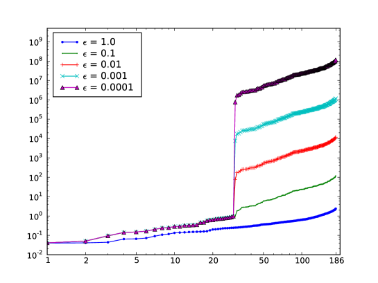
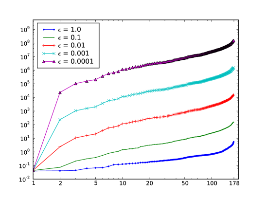
In figures 1 and 2 we illustrate these estimates. Two tetrahedral meshes in a box domain were generated, one which is arranged in horizontal layers, and one which is fully unstructured in all three dimensions. The finite element approximation to the Laplace equation was applied to these meshes, having rescaled the coordinates to various different aspect ratios. The eigenvalues were then numerically computed using Arnoldi iteration. Figure 1 shows the eigenvalues for the layered mesh, with various different aspect ratios. We observe a gap in the spectrum between the eigenvalues corresponding to $z$-independent eigenvectors (we call these horizontal modes) and the eigenvalues corresponding to $z$-dependent eigenvectors. The size of this gap is proportional to $\epsilon^{-2}$. It can also be observed that the ratio between the largest and smallest eigenvalues is proportional to $\epsilon^{-2}$. In the unstructured mesh, the distinction between the horizontal modes and the rest of the eigenvectors is less clear. The lack of horizontal alignment in the mesh means that there are numerical errors in the finite element approximation of the vertical derivatives which scale with the horizontal widths $\Delta x$ of the elements (in this case $\Delta x^{2}$ since we have used linear finite elements) and hence are the same order of magnitude (or larger) than the exact eigenvalues of the horizontal modes. Figure 1 shows the eigenvalues for the unstructured mesh with various different aspect ratios. We observe the same $\epsilon^{-2}$ scaling for the ratio between the largest and smallest eigenvalues, but there is no spectral gap since the small eigenvalues are polluted by numerical errors in the vertical derivatives.

Figure 1: Plot showing eigenvalues for the matrix $A$ arising from the discretisation of the Poisson equation in a box domain with Neumann boundary conditions on all sides. The box was decomposed into a tetrahedral mesh divided into a number of horizontal layers (i.e. the mesh is structured in the vertical) and rescaled into various different aspect ratios $\epsilon$. Note that there are a cluster of small eigenvalues which are independent of $\epsilon$: these eigenvalues correspond to the $z$-independent eigenmodes. As $\epsilon$ decreases to zero, the width of the spectral gap between these and the remaining eigenvalues scales in proportion to $\epsilon^{-2}$.

Figure 2: Plot showing eigenvalues for the matrix $A$ arising from the discretisation of the Poisson equation in a box domain with Neumann boundary conditions on all sides. The box was decomposed into a tetrahedral mesh which is completely unstructured in the vertical and rescaled into various different aspect ratios $\epsilon$. Note that there is no longer a spectral gap, which is replaced by a more evenly spaced spectrum, but that the spread of eigenvalues still increases in proportion to $\epsilon^{-2}$.

In contrast, we note very different scaling behaviour when the Neumann boundary condition on the upper surface (rigid lid) is replaced by a Dirichlet boundary condition, resulting in the matrix $\overline{A}_{\epsilon}$. For this case, we shall obtain an upper bound on the condition number. First we bound the minimum eigenvalue $\overline{\lambda}_{\min}$ of $\overline{A}_{\epsilon}$ from below.

$$\overline{\lambda}_{\min} = \min_{\overline{\boldsymbol{\phi}}\neq\boldsymbol{0}}\frac{\overline{\boldsymbol{\phi}}^{T}\overline{A}_{\epsilon}\overline{\boldsymbol{\phi}}}{\overline{\boldsymbol{\phi}}^{T}\overline{\boldsymbol{\phi}}},$$

$$= \min_{\overline{\boldsymbol{\phi}}\neq\boldsymbol{0}}\frac{\overline{\boldsymbol{\phi}}^{T}\left(\overline{A}_{0}+\epsilon^{2}\overline{A}_{H}\right)\overline{\boldsymbol{\phi}}}{\overline{\boldsymbol{\phi}}^{T}\overline{\boldsymbol{\phi}}},$$

$$\geq \min_{\overline{\boldsymbol{\phi}}\neq\boldsymbol{0}}\frac{\overline{\boldsymbol{\phi}}^{T}\overline{A}_{0}\overline{\boldsymbol{\phi}}}{\overline{\boldsymbol{\phi}}^{T}\overline{\boldsymbol{\phi}}},$$

$$= c_{2},$$

which is the minimum eigenvalue of $\overline{A}_{0}$ and is bounded away from zero since $\overline{A}_{0}$ is non-singular. Next we bound the maximum eigenvalue $\overline{\lambda}_{\max}$ of $\overline{A}_{\epsilon}$.

$$\overline{\lambda}_{\max} = \max_{\overline{\boldsymbol{\phi}}\neq\boldsymbol{0}}\frac{\overline{\boldsymbol{\phi}}^{T}\overline{A}_{\epsilon}\overline{\boldsymbol{\phi}}}{\overline{\boldsymbol{\phi}}^{T}\overline{\boldsymbol{\phi}}},$$

$$= \max_{\overline{\boldsymbol{\phi}}\neq\boldsymbol{0}}\frac{\overline{\boldsymbol{\phi}}^{T}\left(\overline{A}_{0}+\epsilon^{2}\overline{A}_{H}\right)\overline{\boldsymbol{\phi}}}{\overline{\boldsymbol{\phi}}^{T}\overline{\boldsymbol{\phi}}},$$

$$\leq 2\max_{\overline{\boldsymbol{\phi}}\neq\boldsymbol{0}}\frac{\overline{\boldsymbol{\phi}}^{T}\overline{A}_{0}\overline{\boldsymbol{\phi}}}{\overline{\boldsymbol{\phi}}^{T}\overline{\boldsymbol{\phi}}},$$

$$= 2c_{3},$$

provided that $\epsilon$ is sufficiently small; here $c_{3}$ is the maximum eigenvalue of $\overline{A}_{0}$. This means that the condition number of $\overline{A}_{\epsilon}$ is bounded by

$$\operatorname{Cond}(\overline{A}_{\epsilon})=\frac{\overline{\lambda}_{\max}}{\overline{\lambda}_{\min}}\leq\frac{2c_{3}}{c_{2}}=2\operatorname{Cond}(\overline{A}_{0}),$$

which is twice the condition number of $\overline{A}_{0}$, and is independent of $\epsilon$ (this is not a sharp estimate, but illustrates the scaling with $\epsilon$).

The contrast between the condition number scaling of $\overline{A}_{\epsilon}$ and $A_{\epsilon}$ motivates a preconditioner strategy in which one solves a reduced problem for the solution on the surface $\partial\Omega_{\operatorname{\text{top}}}$, and then uses this surface solution as a Dirichlet boundary condition to reconstruct a solution throughout $\Omega$. This reconstruction step amounts to inverting $\overline{A}_{\epsilon}$ which, as we have just seen, has a condition number which is independent of $\epsilon$. We shall describe this preconditioner strategy in the following section.

5 New preconditioner

In this section we develop our new preconditioner for equation (19), which is derived from the strategy of eliminating the degrees of freedom associated with the solution in the interior of $\Omega$ to give a reduced equation on the surface $\partial\Omega_{\operatorname{\text{top}}}$. In each iteration the preconditioner will approximately solve this problem, and then approximately reconstruct the solution in the interior using $\overline{A}_{\epsilon}$. We describe the preconditioner as follows: in Section 5.1 we briefly summarise the general algebraic multigrid preconditioning strategy. In Section 5.2 we introduce a reformulation of equation the (19) that decomposes the inverse of $A$ into a vertically lumped system and a system with a Dirichlet boundary condition on top. Sections 5.3 and 5.4 explain the approximations that need to be made to this decomposition to apply it as a preconditioner.

5.1 Algebraic multigrid preconditioners

The general idea of multigrid methods is to tackle multiscale, ill conditioned problems by trying to solve for the different components of the solution, associated with different length scales, separately. This is accomplished by a sequence of coarsening operations, in which the dimension of the problem is reduced step by step. The coarser system no longer supports the smaller scale features and has therefore an improved condition number. Thus the large scale, small eigenvalue modes can be efficiently solved on a reduced system, whereas the small scale, large eigenvalue modes are easily reduced with standard preconditioners such as SOR (therefore in this context referred to as smoothers).

Classical geometric multigrid methods, implement this coarsening step via a coarsening of the mesh on which the problem is defined, for instance via a $h\to 2h$ coarsening on structured meshes. Algebraic multigrid (AMG) methods (see Stüben (2001) for an introduction), use the algebraic properties, matrix graph and coefficients, of the matrix to construct a coarsening operator. This more general approach has the advantage that it works equally well for unstructured mesh discretisations. Additionally it is possible to take anisotropies in the problem into account by selecting only matrix graph connections associated with large matrix coefficients.

For symmetric problems, to keep the problem symmetric at each level, the prolongation operator $P$, that maps the solution of the reduced system back to the previous level, is usually the transpose of the coarsening operator $P^{T}$. Given the original matrix $A$ at the finest level, the matrix of the reduced system, is given by

$$P^{T}AP\boldsymbol{y}=P^{T}\boldsymbol{b},\qquad\boldsymbol{y}\in\mathbb{R}^{m},$$ (22)

After solving at the coarsest level, the solution is mapped back using $y\to x=Py$.

The smaller scale modes that are only represented in the full problem are reduced by applying a smoother $S$. As this smoothing step will also again change the solution at the coarse level, i.e. the solve at the coarse level and the smoothing for the full problem are not independent, the whole procedure of restriction, coarse solve, prolongation, and smoothing needs to be applied in an iterative manner. To keep things symmetric, the smoothing step $S$ after prolongation is usually mirrored by a transpose smoother $S^{T}$ before the reduction. For instance a forward sweep of SOR before the restriction can be accompanied by a backward sweep after the prolongation.

A typical 2-level multigrid cycle (V-cycle) then looks like

Finally by replacing the coarse solve with a multigrid V-cycle applied to the reduced system, the multigrid method can be extended recursively to multiple levels.

Best results are obtained if the multigrid V-cycle is embedded, as a preconditioner, in a Krylov subspace method. Different multigrid preconditioning approaches are formed by different coarsening strategies and different choices of smoothers. The algebraic multigrid preconditioner used in the results section, implements the smoothed aggregation approach of Vanek et al. (1996). This method is known to work very well for strongly anisotropic elliptic problems. As will be shown in the results section however the convergence rate is not independent of the aspect ratio. Therefore, we seek to improve upon this purely algebraic method in the following sections.

5.2 Schur complement equation

Motivated by the analysis in section 4, where we observed that the condition number of the linear system becomes independent of the aspect ratio if the Neumann boundary condition on top is replaced by a Dirichlet condition, we proceed by constructing a reduced system where we first solve for the solution $\boldsymbol{\phi}^{\prime}$ on $\partial\Omega_{\text{Top}}$, and then reconstruct $\overline{\boldsymbol{\phi}}$ (cf. the decomposition of $\boldsymbol{\phi}$ into $\boldsymbol{\phi}^{\prime}$ and $\boldsymbol{\overline{\phi}}$ in (20) and (21)). This can be done by solving the Schur complement equation

$$\underbrace{(B-C\overline{A}_{\epsilon}^{-1}C^{T})}_{\mbox{Schur matrix}}\boldsymbol{\phi}^{\prime}=\boldsymbol{b}^{\prime}-C\overline{A}_{\epsilon}^{-1}\overline{\boldsymbol{b}},$$ (23)

and then solving

$$\overline{A}_{\epsilon}\overline{\boldsymbol{\phi}}=-C^{T}\boldsymbol{\phi}^{\prime}+\boldsymbol{b}^{\prime},$$ (24)

to reconstruct the solution in the interior. Note that $\dim(\boldsymbol{\phi}^{\prime})\ll\dim(\boldsymbol{\phi})$, and also that the reconstruction equation (24) has a condition number which is independent of $\epsilon$ as $\epsilon\to 0$.

The Schur complement matrix contains $\overline{A}_{\epsilon}^{-1}$ and hence is a full matrix which is expensive to assemble and solve. Hence we shall propose a strategy to form approximations to equations (23) and (24) which can be used as a preconditioner in a manner similar to a multigrid preconditioner.

5.3 Extrapolation operator

To build the approximation to the Schur matrix, we first note that equation 23 may be rewritten as

$$E^{T}A_{\epsilon}E\boldsymbol{\phi}^{\prime}=E^{T}\boldsymbol{b},$$ (25)

where

$$E=\begin{pmatrix}I\\ -\overline{A}_{\epsilon}^{-1}C^{T}\\ \end{pmatrix}.$$

We call $E$ the extrapolation operator. Given $\boldsymbol{\phi}^{\prime}\in\mathbb{R}^{m}$, the operation

$$\boldsymbol{\phi}=E\boldsymbol{\phi}^{\prime},$$

produces the finite element discretisation of the solution of the Laplace equation

$$\nabla^{2}\phi=0,$$ (26)

with Neumann boundary conditions $\partial\psi/\partial n=0$ on the coasts and bottom surface, and Dirichlet boundary conditions

$$\phi=\phi^{\prime}$$ (27)

on the top surface, where $\phi$ is the function on $\Omega$ with finite element basis function coefficient vector $\boldsymbol{\phi}$ and $\phi^{\prime}$ is the function on $\partial\Omega_{\operatorname{\text{top}}}$ with finite element basis function coefficient vector $\boldsymbol{\phi}^{\prime}$. Note that in the small aspect ratio limit, (26) converges to

$$\frac{\partial^{2}}{\partial z^{2}}\phi=0,$$

with $\phi=\phi^{\prime}$ on the top surface, and $\partial\phi/\partial z=0$ on the bottom surface. The solution $\phi$ is then the vertical extrapolation of $\phi^{\prime}$ i.e.

$$\phi(x,y,z)=\phi^{\prime}(x,y).$$

We shall use this in subsequent sections to construct an approximation to $E$.

We can eliminate $\overline{\boldsymbol{\phi}}$ using equation (24) to obtain

$$\boldsymbol{\phi} = \begin{pmatrix}\boldsymbol{\phi}^{\prime}\\ \overline{\boldsymbol{\phi}}\\ \end{pmatrix}$$

$$= \begin{pmatrix}\boldsymbol{\phi}^{\prime}\\ \overline{A}_{\epsilon}^{-1}\left(-C^{T}\boldsymbol{\phi}^{\prime}+\boldsymbol{b}^{\prime}\right)\end{pmatrix}$$

$$= E\boldsymbol{\phi}^{\prime}+\begin{pmatrix}0\\ \overline{A}_{\epsilon}^{-1}\boldsymbol{b}^{\prime}\\ \end{pmatrix}$$

$$= E(E^{T}A_{\epsilon}E)^{-1}E^{T}\boldsymbol{b}+\begin{pmatrix}\boldsymbol{0}\\ I\\ \end{pmatrix}\overline{A}_{\epsilon}^{-1}\begin{pmatrix}\boldsymbol{0}\\ I\\ \end{pmatrix}^{T}\boldsymbol{b},$$

that is

$$A_{\epsilon}^{-1}=\left(E(E^{T}A_{\epsilon}E)^{-1}E^{T}+\underbrace{\begin{pmatrix}\boldsymbol{0}\\ I\\ \end{pmatrix}\overline{A}_{\epsilon}^{-1}\begin{pmatrix}\boldsymbol{0}\\ I\\ \end{pmatrix}^{T}}_{\mathrm{smoother}}\right).$$ (28)

The two parts of this formula may be interpreted in the context of a general multigrid strategy. The first term is similar to a 2-level multigrid cycle with prolongation operator $E$. It projects the equation to a vertically lumped system. The second term acts on the vertical modes in the solution and can therefore be seen as an additive smoother. It is to be noted that (28) provides an exact solution for the inverse of $A_{\epsilon}$, provided both inversions are performed exactly. However, both $E$ and $\overline{A}_{\epsilon}^{-1}$ are dense matrices; in the next two sections we will provide approximations for both the extrapolation operator $E$ and the inverse of $\overline{A}_{\epsilon}$, such that (28) can be used as a preconditioner for equation (19).

Figure 3: Vertical extrapolation performed by projecting each node in the full mesh (here depicted in 2D) straight upward onto the top surface mesh (here 1D), and interpolating the value in this projected node from the surrounding nodes in the surface element.

5.4 Approximation of the vertical extrapolation operator $E$

As noted in the previous section, the operator $E$ given by discretisation of (26) with Dirichlet boundary conditions condition (27) on top, converges to a vertical extrapolation operator as $\epsilon\to 0$. We therefore expect that for large $\epsilon$, such a vertical extrapolation operator, between the top surface mesh and the full mesh, is a good approximation of $E$. This operator can simply be constructed by projecting nodes of the full mesh in the vertical direction onto the surface mesh, and interpolating within the surface triangle each projected node lies (see figure 3). This gives an approximation $\tilde{E}:\mathrm{R}^{m^{\prime}}\to\mathrm{R}^{\overline{m}}$ of $E$ with a limited stencil: for a continuous linear (P1) discretisation in 3 dimensions it connects every interior node with three nodes of the surface mesh.

Another approach to find a sparse approximation of $E$ is given by projecting $E$ onto a chosen sparsity pattern using a modification of the symmetric sparse approximate inverse (SSPAI) (Benzi et al., 1996). $\tilde{E}$ is obtained by writing

$$\tilde{E}=\begin{pmatrix}I\\ F\\ \end{pmatrix}$$

and then selecting a sparsity pattern for $F$. The non sparse entries of $F$ are then obtained by minimising

$$\|F^{T}\overline{A}_{\epsilon}-C\|^{2},$$

subject to the sparsity constraints, where $\|\cdot\|$ is the Frobenius norm. This leads to decoupled sparse matrix problems

$${\overline{A}}_{i}\boldsymbol{v}_{i}=-\boldsymbol{r}_{i},\qquad i=1,\ldots,n,$$

where $\boldsymbol{v}_{i}$ is the $i$-th column of $F$ restricted to the sparsity pattern of that column, $\boldsymbol{r}_{i}$ is the $i$-th column of $C^{T}$ restricted to the sparsity pattern, and $\overline{A}_{i}$ is $\overline{A}_{\epsilon}$ restricted to the sparsity pattern of the $i$-th column. We do not pursue this approach in this paper, preferring to use the projection approach described above.

5.5 Additive smoother

By replacing $E$ with $\tilde{E}$, we have produced the approximate inverse

$$A_{\epsilon}^{-1}\approx\tilde{E}(\tilde{E}^{T}A_{\epsilon}\tilde{E})^{-1}\tilde{E}^{T}+\begin{pmatrix}\boldsymbol{0}\\ I\\ \end{pmatrix}\overline{A}_{\epsilon}^{-1}\begin{pmatrix}\boldsymbol{0}\\ I\\ \end{pmatrix}^{T}.$$ (29)

To use this as a preconditioner, we must also approximate the additive smoother. The second term could be evaluated exactly by solving a matrix equation $\overline{A}_{\epsilon}\overline{\phi}=\overline{b}$ for the interior part of the residual. Although, as noted before, this system is much better conditioned than the full system, the solution of an elliptic equation on the interior of the mesh is still quite an expensive operation that needs to be performed during each application of the preconditioner within each the Krylov iteration. Moreover the solution of this interior equation needs to be done using an iterative Krylov method as well. It is well known that embedding a Krylov method within another Krylov iteration, requires the use of a flexible Krylov method for the outer iteration (e.g. FGMRES (Saad, 1993)). A major drawback would therefore be that this approach would inhibit the use of the Conjugate Gradient method for the outer iteration.

A very simple smoothing strategy is obtained by realising that the first term of the proposed preconditioner is just the first stage of a general multigrid method. In this projection the long scale, horizontal modes are separated out and the vertical projection can therefore be interpreted as a general coarsening step such as those in any multigrid method. The necessary smoothing step to filter out the short scale modes, is there often done by application of one or more SOR iterations of the entire system. For small aspect ratio problems this may therefore be enough to reduce the vertical modes in the error.

In some cases, the mesh may contain a lot of structure in the vertical as well as in the horizontal. For instance an adaptive mesh model might focus resolution on physics related to the baroclinic modes of the system. In such cases the simple SOR smoothing may not be enough. The vertical lumping step would take out too much structure in one step. This may be compared to so called “aggressive coarsening” techniques in general multigrid methods that are usually accompanied with improved smoothing techniques. A more accurate approximation of the second term in (29) would be to replace the inverse matrix $\overline{A}_{\epsilon}^{-1}$ by a full cycle of the general AMG method applied to $\overline{A}_{\epsilon}$. The next section will provide a comparison of the simple SOR smoother with this more advanced additive smoother.

6 Numerical experiments

In this section we present numerical results which test out our preconditioner on matrices obtained from the linear finite element approximation of the Laplace equation with the horizontal coordinates rescaled to various aspect ratios. The solvers were developed using the open source PETSc library (Balay et al., 1997).

To compute errors, we selected a right hand side for the matrix vector equation by choosing a solution and multiplying it by the matrix. This allows us to compute errors exactly at each iteration of the solvers. Throughout this section we use the $\inf$-norm to measure the magnitude of the error: our rationale for this is that we are motivated by multiscale applications in which one may be very concerned with the numerical solution in one small region of the domain (for example one may wish to embed a convection cell in an ocean basin and observe how it is affected by the large scale dynamics). In this case it may be possible to obtain a small $L_{2}$ error whilst the solution in the small region is still inaccurate. We present plots of error against number of iterations, and also against floating point operations (flops). The flop count is provided by a intrinsic PETSc routine.

In this section we obtain results from two meshes, both of a 1$\times$1$\times$1 cube; the coordinates of the meshes are then rescaled to a range of aspect ratios in the small aspect ratio limit. Mesh A is a Delaunay triangulation for a set of 57453 roughly equispaced points in the cube; the points are not arranged in layers and hence the mesh is unstructured in the vertical. Mesh B is a Delaunay triangulation on a mesh in which the majority of the points are clustered at the centre of the cube (there are 99017 points in total), leading to very small elements. This is a truly multiscale mesh in which small eigenvalues exist due to both the small aspect ratio and also due to small elements. Our aim is to develop robust, efficient matrix solvers for these challenging multiscale meshes.

The three preconditioners that are compared are:

• A general AMG method based on the smoothed aggregation method (Vanek et al., 1996). This uses our own implementation constructed using the “MG” interface provided by PETSc. The smoothing at each level is given by a single forward SOR sweep ($\omega=1.0$) as a pre-smoother and a backward sweep for post-smoothing. The coarsening strategy is based on the strongly-coupled connection criterion

  $$|A_{ij}|>\varepsilon\sqrt{A_{ii}A_{jj}}$$

  where a $\varepsilon$ of $0.01$ has been chosen. The smoothing in the aggregation operator uses $\omega=2/3$.

• The preconditioner given by the vertically lumped approach

  $$A_{\epsilon}^{-1}\approx\tilde{E}(\tilde{E}^{T}A_{\epsilon}\tilde{E})^{-1}\tilde{E}^{T}$$

  where the vertically lumped system is approximately solved using a single multigrid cycle applied to $\tilde{E}^{T}A_{\epsilon}\tilde{E}$. This is combined with a single forward and backward SOR sweep as respectively a pre and post smoothing step. Thus the vertical lumping operator $\tilde{E}$ is treated as an ordinary coarsening operator, and the vertical lumping of the equation is simply the first of a multilevel multigrid cycle.

• As a last approach, the above multigrid cycle, including the vertical lumping as the first coarsening step, is combined with the additive smoother, where $\overline{A_{\epsilon}}^{-1}$ is approximated applying a cycle of the smoothed aggregation AMG method to $\overline{A_{\epsilon}}$.

In all cases the full multigrid cycle is applied as a preconditioner within each iteration of the Conjugate Gradient method.

6.1 General multigrid methods

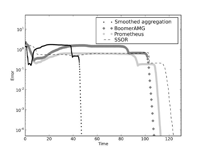
In figure 4, we compare the smoothed aggregation preconditioner to two other algebraic multigrid algorithms available through the PETSc library (BoomerAMG and Prometheus), and the classical Symmetric Successive Over-Relaxation (SSOR) preconditioner. The four preconditioners are combined with the Conjugate Gradient method in solving the pressure Poisson equation on Mesh A rescaled to an aspect ratio of $1/1000$ (a reasonable aspect ratio for large scale oceanographic applications). It is shown that the smoothed aggregation is substantially more effective than the other methods (we additionally notice that the other multigrid methods are not much more effective than SSOR in this small aspect ratio example, although both methods contain a number of parameters and it may be possible to obtain better results by tuning). All four methods produce long “plateaus” in the error that are maintained for many iterations before the error finally drops. This means that none of these preconditioners result in feasible methods for solving the pressure Poisson equation in small aspect ratio domains.

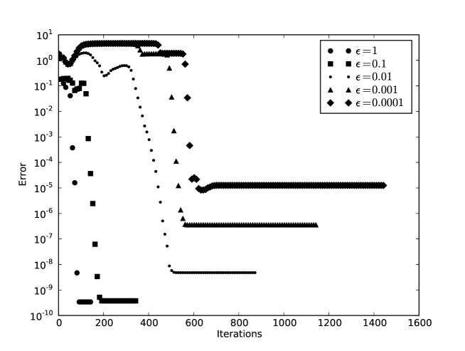
In figure 5, we further illustrate the problems that occur when the Conjugate Gradient method with the smoothed aggregation multigrid preconditioner is applied to the Poisson equation on mesh A. The error is plotted against the iteration number for the preconditioned Conjugate Gradient method for various aspect ratios. As the aspect ratio of the domain decreases, the condition number increases and the convergence rate of the iterative solver gets slower. We observe a “plateau” in the error which is maintained for many iterations before the error finally drops; this plateau becomes longer and longer as the aspect ratio decreases. For small aspect ratios this makes the iterative solver prohibitively slow.

Figure 4: Plot showing error versus computation time for the smoothed aggregation multigrid preconditioner combined with the Conjugate Gradient method, compared with two other multigrid preconditioners available within PETSc (namely BoomerAMG and Prometheus), and the SSOR preconditioner. The smoothed aggregation method uses a coarsening strategy which is weighted by the matrix entries. When the aspect ratio is small (it is $1/1000$ in this case), this method tends to aggregate degrees of freedom which are nearly vertically aligned. The smoothed aggregation method is substantially more effective than the other multigrid methods and the SSOR method, but we still observe a long period during which the error is not reduced.

Figure 5: Plot showing error (using the $\infty$-norm) against number of iterations, for the Conjugate Gradient method applied to the Poisson equation discretised on mesh A, using the smoothed aggregation multigrid preconditioner. The mesh has been rescaled to various different aspect ratios $\epsilon$ as indicated in the plot. The number of iterations required to converge increases with decreasing $\epsilon$, with a long “plateau” for small aspect ratios.

6.2 Preconditioner with vertical lumping

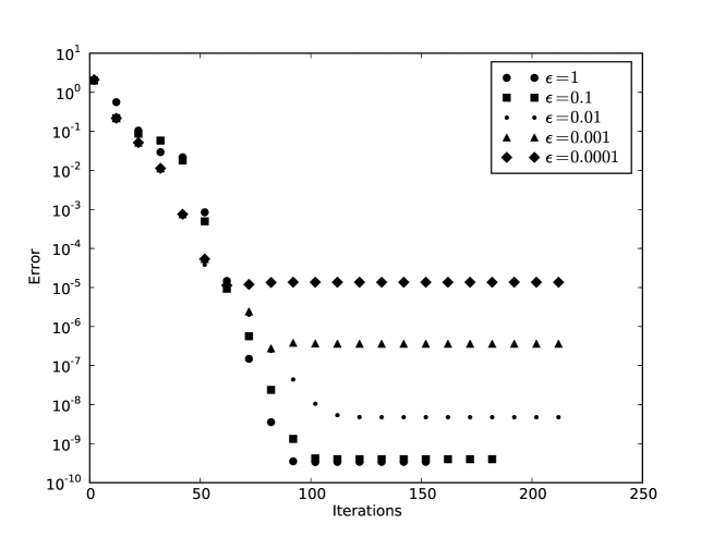
In figure 6, the same information (error plotted against iteration number for the solution of the matrix system obtained from Mesh A) is given for the vertically lumped preconditioner using an SOR smoother. We note that in contrast to the standard multigrid preconditioners tested in the previous subsection, there is no plateau and the convergence rate becomes independent of $\epsilon$ for small aspect ratios. We attribute this fast convergence to the removal of small eigenvalues in (nearly) vertically-independent eigenmodes by the vertically lumped preconditioner. For small aspect ratios there is an exponential decay of error with iteration from the very first iterations.

As an aside, we observe that the remaining error in the approximation after the solver has stopped converging, increases with decreasing $\epsilon$. We ascribe this to numerical round off error (all runs are done in double precision). The scaling of the condition number with $\epsilon$ is consistent with the observed loss in accuracy. The smallest used $\epsilon$ of $0.0001$ still gives an accuracy that is acceptable. This remaining error will show up in all further figures.

Figure 6: Plot showing error (using the $\infty$-norm) against number of iterations, for the Conjugate Gradient method applied to the Poisson equation discretised on mesh A, using the vertically lumped preconditioner. The mesh has been rescaled to various different aspect ratios $\epsilon$ as indicated in the plot. The convergence rate becomes independent of $\epsilon$ for small aspect ratios.

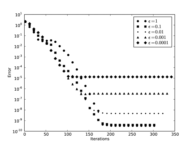
In figure 7, the error is plotted against iteration for the vertically lumped preconditioner using our additive smoother. We note that the error again decays exponentially with iteration number at a rate which is independent of $\epsilon$ for small aspect ratios. However, one sweep of the additive smoother is more expensive than one SOR sweep, and hence it is necessary to compare the performance of the two smoothing strategies in terms of computational cost as well as number of iterations.

Figure 7: Plot showing error (using the $\infty$-norm) against number of iterations, for the Conjugate Gradient method applied to the Poisson equation discretised on mesh A, using the vertically lumped preconditioner combined with additive smoothing. The mesh has been rescaled to various different aspect ratios $\epsilon$ as indicated in the plot. The convergence rate becomes independent of $\epsilon$ for small aspect ratios, but the smoother does not improve the convergence much for this mesh.

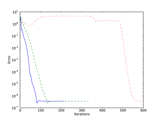
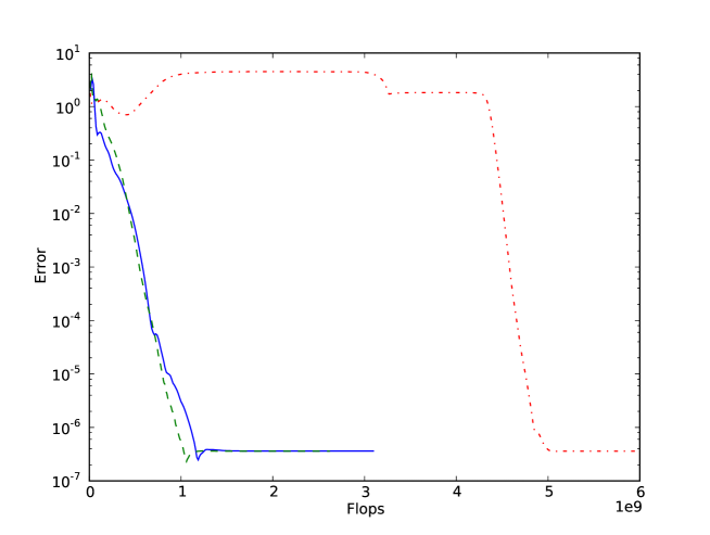
In figure 8, the error is plotted against number of iterations for the smoothed aggregation preconditioner and the vertically lumped preconditioner with and without the additive smoother for the matrix obtained from Mesh A with $\epsilon=0.001$. We observe that the vertically lumped preconditioner converges much faster than the smoothed aggregation preconditioner, and that the additive smoother reduces the number of iterations required for convergence. The vertically lumped preconditioner has made it feasible to solve the pressure Poisson equation on this type of mesh. However, as we observe in figure 9 which shows the error plotted against flops, the additive smoother is more expensive than SOR since it involves several applications of SOR at different levels. We observe that for Mesh A, the time to converge is approximately the same with the SOR smoother or with the additive smoother. The vertically lumped preconditioner produces an approximation to the vertically-independent (barotropic) component of the solution with very small eigenvalues and it is the job of the smoothers to approximate the vertically-varying (baroclinic) component. These results show that for Mesh A, which has roughly isotropic tetrahedra before rescaling to small aspect ratio, the SOR smoother is reasonably effective in approximate the baroclinic components.

Figure 8: Plot showing error (using the $\infty$-norm) against number of iterations, for the Conjugate Gradient method applied to the Poisson equation discretised on mesh A ($\epsilon=0.001$), with various different preconditioners. The continuous line indicates the vertically lumped preconditioner with the additive smoother, the dashed line indicates the vertically lumped preconditioner without the additive smoother, and the dash-dotted line indicates the smoothed aggregation multigrid preconditioner.

Figure 9: Plot showing error (using the $\infty$-norm) against number of floating point operations (flops) counted by PETSc, for the Conjugate Gradient method applied to the Poisson equation discretised on Mesh A ($\epsilon=0.001$), with various different preconditioners. The continuous line indicates the vertically lumped preconditioner with the additive smoother, the dashed line indicates the vertically lumped preconditioner without the additive smoother, and the dash-dotted line indicates the smoothed aggregation multigrid preconditioner.

Figure 10: Plot showing “cutaway” surface through mesh B, used for benchmarking the preconditioner. The mesh has very fine mesh elements at the middle of the domain, so that there are a large range of lengthscales in the mesh.

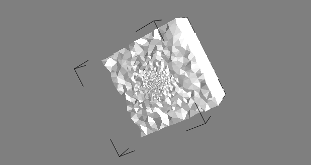
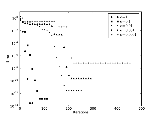
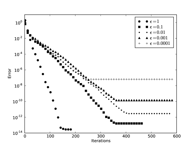
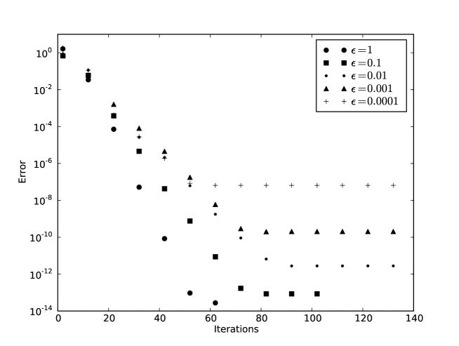
Next we present results for Mesh B which is a multiscale mesh, as illustrated in figure 10. In figure 11, we plot the convergence of the smoothed aggregation multigrid method applied to the matrix obtained from mesh B, which again shows a convergence plateau which becomes longer as $\epsilon\to 0$. Figures 12 and 13 show the convergence rate in iterations for the vertically lumped preconditioner with and without the additive smoother respectively. In both cases the convergence rate becomes independent of $\epsilon$ for small aspect ratios. In this case the additive smoother is producing a faster decay of error as the number of iterations increases, compared to the SOR smoother. This suggests that the additive smoother is more effective at approximating the baroclinic components of the solution, which have a complex multiscale structure. The additive smoother uses an algebraic multigrid cycle applied to the baroclinic components, which operates at several scales simultaneously.

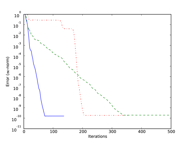
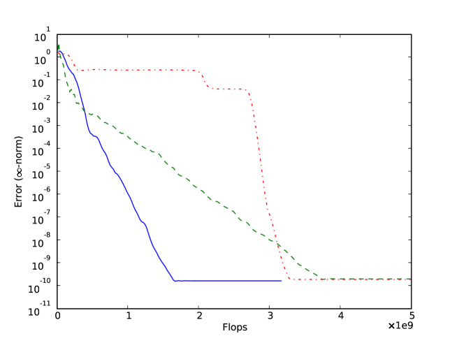
Finally in figure 14, the error is plotted against number of iterations for the smoothed aggregation preconditioner and the vertically lumped preconditioner with and without the additive smoother for the matrix obtained from Mesh B with $\epsilon=0.001$. We observe again that the vertically lumped preconditioner converges much faster than the smoothed aggregation preconditioner. Here the vertically lumped preconditioner does not exhibit a convergence plateau but does have a slow rate of convergence which we attribute to the presence of the small eigenvalues associated with small scales in the mesh which are not altered by the vertically lumped preconditioner. The inclusion of the additive smoother means that the number of iterations is dramatically reduced, since the additive smoother is a multigrid preconditioner which treats all of the scales in the mesh. Despite the added cost of the additive smoother, we observe that it results in a much more efficient solver. We conclude that the additive smoother should be used when small scales are present in the mesh which lead to eigenvalues which are of the same size as those associated with eigenvectors corresponding to horizontal modes.

Figure 11: Plot showing error (using the $\infty$-norm) against number of iterations, for the Conjugate Gradient method applied to the Poisson equation discretised on mesh B (shown in figure 10, $\epsilon=0.001$), using the smoothed aggregation multigrid preconditioner. The mesh has been rescaled to various different aspect ratios $\epsilon$ as indicated in the plot. The number of iterations required to converge increases for decreasing $\epsilon$, with a long “plateau” for small aspect ratios.

Figure 12: Plot showing error (using the $\infty$-norm) against number of iterations, for the Conjugate Gradient method applied to the Poisson equation discretised on mesh B (shown in figure 10, $\epsilon=0.001$), using the vertically lumped preconditioner. The mesh has been rescaled to various different aspect ratios $\epsilon$ as indicated in the plot. The convergence rate becomes independent of $\epsilon$ for small aspect ratios.

Figure 13: Plot showing error (using the $\infty$-norm) against number of iterations, for the Conjugate Gradient method applied to the Poisson equation discretised on mesh B (shown in figure 10), using the vertically lumped preconditioner combined with additive smoothing. The mesh has been rescaled to various different aspect ratios $\epsilon$ as indicated in the plot. The convergence rate becomes independent of $\epsilon$ for small aspect ratios, with a substantial improvement over the vertically lumped preconditioner with standard SOR smoothing, shown in figure 12.

Figure 14: Plot showing error (using the $\infty$-norm) against number of iterations, for the Conjugate Gradient method applied to the Poisson equation discretised on mesh B (shown in figure 10), with various different preconditioners. The continuous line indicates the vertically lumped preconditioner with the additive smoother, the dashed line indicates the vertically lumped preconditioner without the additive smoother, and the dash dotted line indicates the smoothed aggregation multigrid preconditioner.

Figure 15: Plot showing error (using the $\infty$-norm) against number of floating point operations (flops) counted by PETSc, for the Conjugate Gradient method applied to the Poisson equation discretised on Mesh B (shown in figure 10), with various different preconditioners. The continuous line indicates the vertically lumped preconditioner with the additive smoother, the dashed line indicates the vertically lumped preconditioner without the additive smoother, and the dash dotted line indicates the smoothed aggregation multigrid preconditioner.

7 Summary and outlook

In this paper we discussed the ill conditioning of the linear system obtained from the finite element approximation of the pressure Poisson equation on general vertically unstructured meshes in small aspect ratio domains (such as the global oceans). We showed that the condition number scales like $\epsilon^{-2}$ as $\epsilon\to 0$ (where $\epsilon$ is the aspect ratio $H/L$) in the case in which Neumann boundary conditions are set on all surfaces. We also showed that the condition number is independent of $\epsilon$ when Dirichlet conditions are applied at the top surface. This motivated a preconditioner consisting of two stages: in the first stage an approximate reduced system for the surface degrees of freedom is solved, and in the second stage the solution is reconstructed throughout the domain with the approximate surface solution used as a Dirichlet boundary condition. The first stage results in a much smaller linear system, and the second stage involves a submatrix which has a condition number which is independent of $\epsilon$. The reduced system is obtained using an algebraic multigrid prolongation operator which approximates the vertical extrapolation operator, and the second stage submatrix can be solved using further algebraic multigrid stages. Using numerical experiments, we showed that this preconditioner, when combined with the Conjugate Gradient method, results in a solver which has a convergence rate that is independent of the aspect ratio. Further, we showed that the additional computational cost of using the additive smoother means that it is only beneficial in truly multiscale meshes. Those are meshes that do not just have two entirely different lenght scales, the horizontal and the vertical, but a whole range of scales inbetween . This strategy will become crucial when solving process study problems consisting of small scale dynamics (such as open ocean deep convection, or density overflows) that are embedded in a large scale circulation. We also anticipate that the smoother will become important when parallel domain decomposition methods are used, where (block) SOR smoothing methods are known to be less effective. The methods described in this paper have been implemented in ICOM where they will be used to investigate adaptive unstructured large scale ocean modelling.

8 Acknowledgements

The authors would like to acknowledge the funding of the UK Natural Environment Research Council under grant NE/C52101X/1, and of Fujitsu Laboratories of Europe.

References

- Balay et al. (1997) Balay, S., Gropp, W. D., McInnes, L. C., Smith, B. F., 1997. Efficient management of parallelism in object oriented numerical software libraries. In: Arge, E., Bruaset, A. M., Langtangen, H. P. (Eds.), Modern Software Tools in Scientific Computing. Birkhäuser Press, pp. 163–202.
- Benzi et al. (1996) Benzi, M., Meyer, C. D., Tuma, M., 1996. A sparse approximate inverse preconditioner for the conjugate gradient method. SIAM Journal on Scientific Computing 17 (5), 1135–1149.
- Bochev and Lehoucq (2005) Bochev, P., Lehoucq, R. B., 2005. On the finite element solution of the pure Neumann problem. SIAM Review 47 (1), 50–66.
- Brenner and Scott (1994) Brenner, S., Scott, R., 1994. The Mathematical Theory of Finite Element Methods. Springer-Verlag.
- Chorin (1967) Chorin, A. J., 1967. The numerical solution of the Navier-Stokes equations for an incompressible fluid. Bull. Amer. Math. Soc. 73 (6), 928–931.
- Fringer et al. (2006) Fringer, O. B., Gerritsen, M., Street, R. L., 2006. An unstructured-grid, finite-volume, nonhydrostatic, parallel coastal-ocean simulator. Ocean Modelling 14 (3-4), 139–278.
- Gresho and Sani (2000) Gresho, P. M., Sani, R. L., 2000. Incompressible Flow and the Finite Element Method, Volume 2, Isothermal Laminar Flow. Wiley.
- Holm et al. (1998) Holm, D. D., Marsden, J. E., Ratiu, T. S., 1998. The Euler–Poincaré equations and semidirect products with applications to continuum theories. Adv. in Math. 137, 1–81.
- Karniadakis and Sherwin (2005) Karniadakis, G. E. M., Sherwin, S., 2005. Spectral/hp Element Methods for Computational Fluid Dynamics. Oxford Science Publications, Ch. 7.
- Labeur and Pietrzak (2005) Labeur, R. J., Pietrzak, J. D., 2005. A fully three dimensional unstructured grid non-hydrostatic finite element coastal model. Ocean Modelling 10 (1-2), 51–67, the Second International Workshop on Unstructured Mesh Numerical Modelling of Coastal, Shelf and Ocean Flows.
- Marshall et al. (1997) Marshall, J., Adcroft, A., Hill, C., Perelman, L., Heisey, C., 1997. A finite-volume, incompressible Navier Stokes model for studies of the ocean on parallel computers. Journal of Geophysical Research 102, 5753–5766.
- Pain et al. (2005) Pain, C., Piggott, M., Goddard, A., Fang, F., Gorman, G., Marshall, D., Eaton, M., Power, P., de Oliveira, C., 2005. Three-dimensional unstructured mesh ocean modelling. Ocean Modelling 10 (1-2), 5 – 33.
- Pedlosky (1987) Pedlosky, J., 1987. Geophysical Fluid Dynamics, 2nd Edition. Springer.
- Piggott et al. (2008) Piggott, M. D., Gorman, G. J., Pain, C. C., Allison, P. A., Candy, A. S., Martin, B. T., Wells, M. R., 2008. A new computational framework for multi-scale ocean modelling based on adapting unstructured meshes. International Journal for Numerical Methods in Fluids 56 (8), 1003–1015.
- Saad (1993) Saad, Y., 1993. A flexible inner-outer preconditioned gmres algorithm. SIAM J. Sci. Comput. 14 (2), 461–469.
- Shchepetkin and McWilliams (2005) Shchepetkin, A. F., McWilliams, J., 2005. The Regional Ocean Modeling System (ROMS): A split-explicit, free-surface, topography-following coordinates ocean model. Ocean Modelling 9, 347–404.
- Shewchuk (1994) Shewchuk, J. R., 1994. An introduction to the conjugate gradient method without the agonizing pain, www.cs.cmu.edu/ quake-papers/painless-conjugate-gradient.pdf.
- Stüben (2001) Stüben, K., 2001. A review of algebraic multigrid. J. Comput. Appl. Math. 128, 281.
- Temam (1969) Temam, R., 1969. Sur l’approximation de la solution des équations de Navier-Stokes par la méthode des pas fractionnaires (ii). Arch. Rational Mech. Anal. 33 (377–385).
- Vanek et al. (1996) Vanek, P., Mandel, J., Brezina, M., 1996. Algebraic multigrid by smoothed aggregation for second and fourth order elliptic problems. Computing 56, 179–196.