Multiplicative Noise Removal Using Variable Splitting and Constrained Optimization

Abstract

Multiplicative noise (also known as speckle noise) models are central to the study of coherent imaging systems, such as synthetic aperture radar and sonar, and ultrasound and laser imaging. These models introduce two additional layers of difficulties with respect to the standard Gaussian additive noise scenario: (1) the noise is multiplied by (rather than added to) the original image; (2) the noise is not Gaussian, with Rayleigh and Gamma being commonly used densities. These two features of multiplicative noise models preclude the direct application of most state-of-the-art algorithms, which are designed for solving unconstrained optimization problems where the objective has two terms: a quadratic data term (log-likelihood), reflecting the additive and Gaussian nature of the noise, plus a convex (possibly nonsmooth) regularizer (e.g., a total variation or wavelet-based regularizer/prior). In this paper, we address these difficulties by: (1) converting the multiplicative model into an additive one by taking logarithms, as proposed by some other authors; (2) using variable splitting to obtain an equivalent constrained problem; and (3) dealing with this optimization problem using the augmented Lagrangian framework. A set of experiments shows that the proposed method, which we name MIDAL (multiplicative image denoising by augmented Lagrangian), yields state-of-the-art results both in terms of speed and denoising performance.

I Introduction

Many special purpose imaging systems use coherent demodulation of reflected electromagnetic or acoustic waves; well known examples include ultrasound imaging, synthetic aperture radar (SAR) and sonar (SAS), and laser imaging. Due to the coherent nature of these image acquisition processes, the standard additive Gaussian noise model, so prevalent in image processing, is inadequate. Instead, multiplicative noise models, i.e., in which the noise field is multiplied by (not added to) the original image, provide an accurate description of these coherent imaging systems. In these models, the noise field is described by a non-Gaussian probability density function, with Rayleigh and Gamma being common models.

In this introductory section, we begin by briefly recalling how coherent imaging acquisition processes lead to multiplicative noise models; for a more detailed coverage of this topic, the reader is referred to [24], [25], [31], [34]. We then review previous approaches for dealing with images affected by multiplicative noise and finally briefly describe the approach proposed in this paper.

I-A Coherent Imaging and Multiplicative Noise

With respect to a given resolution cell of the imaging device, a coherent system acquires the so-called in-phase and quadrature components, which are the outputs of two demodulators with respect to, respectively, $\cos(\omega t)$ and $\sin(\omega t)$, where $\omega$ is the angular frequency of the carrier signal. Usually, these two components are collected into a complex number, with the in-phase and quadrature components corresponding to the real and imaginary parts, respectively [24]. The complex observation from a given resolution cell results from the contributions of all the individual scatterers present in that cell, which interfere in a destructive or constructive manner, according to their spatial configuration. When this configuration is random, it yields random fluctuations of the complex observation, a phenomenon which is usually referred to as speckle. The statistical properties of speckle have been widely studied and are the topic of a large body of literature [24], [25], [29], [31].

Assuming a large number of randomly distributed scatterers and no strong specular reflectors in each resolution cell the complex observation is well modeled by a zero-mean complex Gaussian circular density (i.e., the real and imaginary parts are independent Gaussian variables with a common variance). Consequently, the magnitude of this complex observation follows a Rayleigh distribution and the square of the magnitude (the so-called intensity) is exponentially distributed [29], [31]. The term multiplicative noise is clear from the following observation: an exponential random variable can be written as the product of its mean value, the so-called reflectance (the parameter of interest to be estimated) by an exponential variable of unit mean (the noise).

The scenario just described, known as fully developed speckle, leads to observed intensity images with a characteristic granular appearance, due to the very low signal to noise ratio (SNR). Notice that the SNR, defined as the ratio between the squared intensity mean and the intensity variance, is equal to one ($0\,$dB); this is a consequence of the equality between the mean and the standard deviation of an exponential distribution.

I-B Improving the SNR: Multi-look Acquisition

A common approach to improving the SNR in coherent imaging consists in averaging independent observations of the same resolution cell (pixel). In SAR/SAS systems, this procedure is called multi-look ($M$-look, in the case of $M$ looks), and each independent observation may be obtained by a different segment of the sensor array. For fully developed speckle, the resulting averages are Gamma distributed and the SNR of an $M$-look image is improved to $M$.

Another way to obtain an M-look image is to apply a low pass spatial filter (with a moving average kernel with support size $M$) to a 1-look fully developed speckle image, making evident the tradeoff between SNR and spatial resolution. This type of $M$-look image can be understood as an estimate of the underlying reflectance, under the assumption that this reflectance is constant in the set of cells (pixels) included in the averaging process. A great deal of research has been devoted to developing space variant filters which average large numbers of pixels in homogeneous regions, yet avoid smoothing across reflectance discontinuities, in order to preserve details/edges [20]. Many other speckle reduction techniques have been proposed; see [31] for a comprehensive review of the literature up to 1998.

I-C Estimation of Reflectance: Variational Approaches

What is usually referred to as multiplicative noise removal is of course nothing but the estimation of the reflectance of the underlying scene. This is an inverse problem calling for regularization, which usually consists in assuming that the underlying reflectance image is piecewise smooth. In image denoising under multiplicative noise, this assumption has been formalized, in a Bayesian estimation framework, using Markov random field priors [7], [31]. More recently, variational approaches using total variation (TV) regularization were proposed [1], [27], [34], [37], [38]. In a way, these approaches extend the spatial filtering methods referred to in the previous subsection; instead of explicitly piecewise flat estimates, these approaches yield piecewise smooth estimates adapted to the structure of the underlying reflectance.

Both the variational and the Bayesian maximum a posteriori (MAP) formulations to image denoising (under multiplicative, Gaussian, or other noise models) lead to optimization problems with two terms: a data fidelity term (log-likelihood) and a regularizer (log-prior). Whereas in Gaussian noise models, the data fidelity term is quadratic, thus quite benign from an optimization point of view, the same is no longer true under multiplicative observations. In [1], the data fidelity term is the negative log-likelihood resulting directly from the $M$-look multiplicative model, which, being non-convex, raises difficulties from an optimization point of view. Another class of approaches, which is the one adopted in this paper, also uses the $M$-look multiplicative model, but yields convex data fidelity terms by formulating the problem with respect to the logarithm of the reflectance; see [15], [27], [34], [37], [38], and references therein. A detailed analysis of several data fidelity terms for the multiplicative noise model can be found in [38].

The combination of TV regularization with the log-likelihood resulting from the multiplicative observation model leads to an objective function, with a non-quadratic term (the log-likelihood) plus a non-smooth term (the TV regularizer), to which some research work has been recently devoted [1], [27], [34], [37], [38]. Even when the log-likelihood is convex (as in [27], [34], [37], [38]), it does not have a Lipschitz-continuous gradient, which is a necessary condition for the applicability (with guaranteed convergence) of algorithms of the forward-backward splitting (FBS) class [3], [6], [13], [41]. Methods based on the Douglas-Rachford splitting (DRS), which do not require the objective function to have a Lipschitz-continuous gradient, have been recently proposed [12], [38].

I-D Proposed Approach

In this paper we address the (unconstrained) convex optimization problem which results from the $M$-look multiplicative model formulated with respect to the logarithm of the reflectance. As shown in [38], this is the most adequate formulation to address reflectance estimation under multiplicative noise with TV regularization. We propose an optimization algorithm with the following building blocks:

• the original unconstrained optimization problem is first transformed into an equivalent constrained problem, via a variable splitting procedure;

• this constrained problem is then addressed using an augmented Lagrangian method.

This paper is an elaboration of our previous work [5], where we have addressed multiplicative noise removal also via a variable splitting procedure. In that paper, the constrained optimization problem was dealt with by exploiting the recent split-Bregman approach [23], but using a splitting strategy which is quite different from the one in [23].

It happens that the Bregman iterative methods recently proposed to handle imaging inverse problems are equivalent to augmented Lagrangian (AL) methods [30], as shown in [42]. We prefer the AL perspective, rather than the Bregman iterative view, as it is a standard and more elementary optimization tool (covered in most textbooks on optimization). In particular, we solve the constrained problem resulting from the variable splitting using an algorithm (of the AL family) known as alternating direction method of multipliers (ADMM) [16], [21], [22].

Other authors have recently addressed the variational restoration of speckled images [1], [12], [27], [34], [37], [38]. The commonalities and differences between our approach and the approaches followed by other authors will be discussed after the detailed description of our method, since this discussion requires notation and concepts which will be introduced in the next section.

The paper is organized as follows. Section II formulates the problem, including the detailed description of the multiplicative noise model and the TV regularization we adopt to estimate the reflectance image. Section III reviews the variable splitting and the augmented Lagrangian optimization methods, which are the basic tools with which our approach is built. Section IV introduces the proposed algorithm by direct application of the basic tools introduced in Section III. Section V discusses related work. Section VI reports the results of a series of experiments aiming at comparing the proposed algorithm with previous state-of-the-art competitors. Finally, Section VII concludes the paper.

II Problem Formulation

Let ${\bf y}\in\mathbb{R}_{+}^{n}$ denote an $n$-pixel observed image, assumed to be a sample of a random image ${\bf Y}$, the mean of which is the underlying (unknown) reflectance image ${\bf x}\in\mathbb{R}_{+}^{n}$, that is, $\mathbb{E}[{\bf Y}]={\bf x}$. Adopting a conditionally independent multiplicative noise model, we have

$$Y_{i}=x_{i}\,N_{i},\;\;\mbox{for\ $\;i=1,...,n$,}$$ (1)

where ${\bf N}\in\mathbb{R}_{+}^{n}$ is an image of independent and identically distributed (iid) random variables with unit mean, $\mathbb{E}(N_{i})=1$, following a common probability density function $p_{N}$. In the case of $M$-look fully developed speckle noise, $p_{N}$ is a Gamma density

$$p_{N}(n)=\frac{M^{M}}{\Gamma(M)}\;n^{M-1}e^{-nM},$$ (2)

thus with expected value $\mathbb{E}[N]=1$ and variance

$$\sigma_{N}^{2}\equiv\mathbb{E}\left[(N-\mathbb{E}[N])^{2}\right]=\frac{1}{M}.$$

Accordingly, we define the signal-to-noise ratio (SNR) associated to a random variable $Y_{i}$, for $i=1,\dots,n$, as

$$\mbox{SNR}\equiv\frac{\mathbb{E}[Y_{i}]^{2}}{\sigma^{2}_{Y_{i}}}=M.$$ (3)

An additive noise model is obtained by taking logarithms of (1) [15], [27], [34], [37], [38]. For an arbitrary pixel of the image (thus dropping the pixel subscript for simplicity), the observation model becomes

$$\underbrace{\log Y}_{G}=\underbrace{\log x}_{z}+\underbrace{\log N}_{W}.$$ (4)

The density of the random variable $W=\log N$ is

$$p_{W}(w) = p_{N}(e^{w})\,e^{w}$$ (5)

$$= \frac{M^{M}}{\Gamma(M)}\;e^{Mw}e^{-e^{w}M},$$

thus

$$p_{G|z}(g|z)=p_{W}(g-z).$$ (6)

Invoking the conditional independence assumption, we are finally lead to

$$\log p_{{\bf G}|{\bf z}}({\bf g}|{\bf z}) = \sum_{s=1}^{n}\log p_{W}(g_{s}-z_{s})$$ (7)

$$= C-M\sum_{s=1}^{n}(z_{s}+e^{\,g_{s}-z_{s}}),$$ (8)

where $C$ is a constant (irrelevant for estimation purposes).

Using the MAP criterion (which is equivalent to a regularization method), the original image is inferred by solving an unconstrained minimization problem with the form

$$\widehat{{\bf z}}\in\arg\min_{{\bf z}}L({\bf z}),$$ (9)

where $L({\bf z})$ is the objective function given by

$$L({\bf z}) = -\log p_{{\bf G}|{\bf Z}}({\bf g}|{\bf z})+\lambda\,\phi({\bf z}).$$ (10)

$$= M\sum_{s=1}^{n}\left(z_{s}+e^{g_{s}-z_{s}}\right)+\lambda\,\phi({\bf z})+A;$$ (11)

in (11), $A$ is an irrelevant additive constant, $\phi$ is the negative of the log-prior (the regularizer), and $\lambda$ is the so-called regularization parameter.

In this work, we adopt the standard isotropic discrete TV regularizer [8], that is,

$$\phi({\bf z})\equiv\sum_{s=1}^{n}\sqrt{(\Delta^{h}_{s}{\bf z})^{2}+(\Delta^{v}_{s}{\bf z})^{2}},$$ (12)

where $\Delta^{h}_{s}{\bf z}$ and $\Delta^{v}_{s}{\bf z}$ denote the horizontal and vertical first order differences at pixel $s\in\{1,\dots,n\}$, respectively.

Each term $\left(z_{s}+e^{g_{s}-z_{s}}\right)$ of (11), corresponding to the negative log-likelihood, is strictly convex and coercive, thus so is their sum. Since the TV regularizer is also convex (though not strictly so), the objective function $L$ possesses a unique minimizer [13], which is a fundamental property, in terms of optimization. In contrast, the formulation of the problem in terms of the original variables ${\bf x}$ (rather than their logarithm) leads to a non-convex optimization problem [1], [34]. As seen in [1], the uniqueness of the minimizer of that non-convex objective is not guaranteed in general.

In this paper, we will address problem (9) using variable splitting and augmented Lagrangian optimization. In the next section, we briefly review these tools, before presenting our approach in detail.

III Basic Tools

III-A Variable Splitting

Consider an unconstrained optimization problem in which the objective function is the sum of two functions, one of which is written as a composition:

$$\min_{{\bf u}\in\mathbb{R}^{n}}f_{1}({\bf u})+f_{2}\left(g({\bf u})\right).$$ (13)

Variable splitting is a very simple procedure that consists in creating a new variable, say ${\bf v}$, to serve as the argument of $f_{2}$, under the constraint that $g({\bf u})={\bf v}$. The idea is to consider the constrained problem

$$\begin{array}[]{cl}{\displaystyle\min_{{\bf u},{\bf v}\in\mathbb{R}^{n}}}&f_{1}({\bf u})+f_{2}({\bf v})\\ \mbox{s.t.}&g({\bf u})={\bf v},\end{array}$$ (14)

which is clearly equivalent to unconstrained problem (13). Notice that in the feasible set $\{({\bf u},{\bf v}):g({\bf u})={\bf v}\}$, the objective function in (14) coincides with that in (13).

The rationale behind variable splitting methods is that it may be easier to solve the constrained problem (14) than it is to solve its unconstrained counterpart (13). This idea has been recently used in several image processing applications [4], [23], [27], [40].

A variable splitting method was used in [40] to obtain a fast algorithm for TV-based image restoration. Variable splitting was also used in [4] to handle problems involving compound regularizers; i.e., where instead of a single regularizer $\lambda\phi$ as in (11), one has a linear combination of two (or more) regularizers $\lambda_{1}\phi_{1}+\lambda_{2}\phi_{2}$. In [4], [27], and [40], the constrained problem (14) is attacked by a quadratic penalty approach, i.e., by solving

$$\min_{{\bf u},{\bf v}\in\mathbb{R}^{n}}f_{1}({\bf u})+f_{2}({\bf v})+\frac{\mu}{2}\,\|g({\bf u})-{\bf v}\|_{2}^{2},$$ (15)

by alternating minimization with respect to ${\bf u}$ and ${\bf v}$, while slowly taking $\mu$ to very large values (a continuation process), to force the solution of (15) to approach that of (14), which in turn is equivalent to (13). The rationale behind these methods is that each step of this alternating minimization may be much easier than the original unconstrained problem (13). The drawback is that as $\mu$ becomes very large, the intermediate minimization problems become increasingly ill-conditioned, thus causing numerical problems (see [30], Chapter 17).

A similar variable splitting approach underlies the recently proposed split-Bregman methods [23]; however, instead of using a quadratic penalty technique, those methods attack the constrained problem directly using a Bregman iterative algorithm [42]. It has been shown that, when $g$ is a linear function, i.e., the constraints in (14) are linear (e.g., $g({\bf u})={\bf Gu}$), the Bregman iterative algorithm is equivalent to the augmented Lagrangian method [42], which is briefly reviewed in the following subsection.

III-B Augmented Lagrangian

In this brief presentation of the augmented Lagrangian method, we closely follow [30], which the reader should consult for more details. Consider an equality constrained optimization problem (which includes (14) as a particular instance, if $g$ is linear)

$$\begin{array}[]{cl}{\displaystyle\min_{{\bf z}\in\mathbb{R}^{d}}}&E({\bf z})\\ \mbox{s.t.}&{\bf Az-b=}\mbox{\boldmath$0$},\end{array}$$ (16)

where ${\bf b}\in\mathbb{R}^{p}$ and ${\bf A}\in\mathbb{R}^{p\times d}$, i.e., there are $p$ linear equality constraints. The so-called augmented Lagrangian function for this problem is defined as

$${\cal L}_{A}({\bf z},\mbox{\boldmath$\lambda$},\mu)=E({\bf z})+\mbox{\boldmath$\lambda$}^{T}({\bf Az-b})+\frac{\mu}{2}\,\|{\bf Az-b}\|_{2}^{2},$$ (17)

where $\mbox{\boldmath$\lambda$}\in\mathbb{R}^{p}$ is a vector of Lagrange multipliers and $\mu\geq 0$ is the penalty parameter.

The so-called augmented Lagrangian method (ALM), also known as the method of multipliers [26], [33], consists in minimizing ${\cal L}_{A}({\bf z},\mbox{\boldmath$\lambda$},\mu)$ with respect to ${\bf z}$, keeping $\lambda$ fixed, and then updating $\lambda$.

• Set $k=0$, choose $\mu>0$, and $\mbox{\boldmath$\lambda$}_{0}$.

• repeat

• ${\bf z}_{k+1}\in\arg\min_{{\bf z}}{\cal L}_{A}({\bf z},\mbox{\boldmath$\lambda$}_{k},\mu)$

• $\mbox{\boldmath$\lambda$}_{k+1}\leftarrow\mbox{\boldmath$\lambda$}_{k}+\mu({\bf Az}_{k+1}-{\bf b})$

• $k\leftarrow k+1$

• until stopping criterion is satisfied.

Although it is possible (even recommended) to update the value of $\mu$ in each iteration [2], [30], we will not consider that option in this paper. Importantly, unlike in the quadratic penalty method, it is not necessary to take $\mu$ to infinity to guarantee that the ALM converges to the solution of the constrained problem (16).

Notice that (after a straightforward complete-the-squares procedure) the terms added to $E({\bf z})$ in the definition of the augmented Lagrangian ${\cal L}_{A}({\bf z},\mbox{\boldmath$\lambda$},\mu)$ in (17) can be written as a single quadratic term, leading to the following alternative form for the ALM algorithm:

• Set $k=0$, choose $\mu>0$, ${\bf z}_{0}$, and ${\bf d}_{0}$.

• repeat

• ${\bf z}_{k+1}\in\arg\min_{{\bf z}}E({\bf z})+\frac{\mu}{2}\|{\bf Az-d}_{k}\|_{2}^{2}$

• ${\bf d}_{k+1}\leftarrow{\bf d}_{k}-({\bf Az}_{k+1}-{\bf b})$

• $k\leftarrow k+1$

• until stopping criterion is satisfied.

This form of the ALM algorithm makes clear its equivalence with the Bregman iterative method (see [42]).

It has been shown that, with adequate initializations, the ALM algorithm generates the same sequence as a proximal point algorithm (PPA) applied to the Lagrange dual of problem (16); for further details, see [28], [35], and references therein. Moreover, the sequence $\{{\bf d}_{k}\}$ converges to a solution of this dual problem and that all cluster points of the sequence $\{{\bf z}_{k}\}$ are solutions of the (primal) problem (16) [28].

III-C Augmented Lagrangian for Variable Splitting

We now show how ALM can be used to address problem (14), in the particular case where $g({\bf u})\equiv{\bf u}$ (i.e., $g$ is the identity function). This problem can be written in the form (16) using the following definitions:

$${\bf z}\equiv\left[\!\begin{array}[]{c}{\bf u}\\ {\bf v}\end{array}\!\right],\hskip 14.22636pt{\bf b}\equiv{\bf 0},\hskip 14.22636pt{\bf A}\equiv[\,{\bf I}\;\;-{\bf I}\,],$$ (18)

and

$$E({\bf z})\equiv f_{1}({\bf u})+f_{2}({\bf v}).$$ (19)

With these definitions in place, steps 3 and 4 of the ALM (version II) can be written as follows

$$\left[\!\!\!\begin{array}[]{c}{\bf u}_{k+1}\\ {\bf v}_{k+1}\end{array}\!\!\!\right]\!\! \!\!\in\!\! \!\!\arg\min_{{\bf u},{\bf v}}\left\{\!f_{1}({\bf u})\!+\!f_{2}({\bf v})\!+\!\frac{\mu}{2}\|{\bf u}\!-\!{\bf v}\!-\!{\bf d}_{k}\|_{2}^{2}\right\}\hskip 11.38092pt$$ (22)

$${\bf d}_{k+1}\!\! \!\!\leftarrow\!\! \!\!{\bf d}_{k}-({\bf u}_{k+1}-{\bf v}_{k+1}).$$ (23)

The minimization (22) is not trivial since, in general, it involves non-separable quadratic and possibly non-smooth terms. A natural solution is to use a non-linear block-Gauss-Seidel (NLBGS) technique, in which (22) is solved by alternating minimization with respect to ${\bf u}$ and ${\bf v}$. Of course this raises several questions: for a given ${\bf d}_{k}$, how much computational effort should be spent in approximating the solution of (22)? Does this NLBGS procedure converge? Taking just one step of this NLBGS scheme in each iteration of ALM leads to an algorithm known as the alternating direction method of multipliers (ADMM) [16], [21], [22] (see also [17], [35], [38]):

• Set $k=0$, choose $\mu>0$, ${\bf v}_{0}$, and ${\bf d}_{0}$.

• repeat

• ${\bf u}_{k+1}\in\arg\min_{{\bf u}}f_{1}({\bf u})+\frac{\mu}{2}\|{\bf u}-{\bf v}_{k}-{\bf d}_{k}\|_{2}^{2}$

• ${\bf v}_{k+1}\in\arg\min_{{\bf v}}f_{2}({\bf v})+\frac{\mu}{2}\|{\bf u}_{k+1}-{\bf v}-{\bf d}_{k}\|_{2}^{2}$

• ${\bf d}_{k+1}\leftarrow{\bf d}_{k}-({\bf u}_{k+1}-{\bf v}_{k+1}-{\bf b})$

• $k\leftarrow k+1$

• until stopping criterion is satisfied.

For later reference, we now recall the theorem by Eckstein and Bertsekas [16] in which convergence of (a generalized version of) ADMM is shown. This theorem applies to problems of the form (13) with $g({\bf u})\equiv{\bf G}{\bf u}$, i.e.,

$$\min_{{\bf u}\in\mathbb{R}^{n}}f_{1}({\bf u})+f_{2}\left({\bf G\,u}\right),$$ (24)

of which (14) is the constrained optimization reformulation.

Theorem 1 (Eckstein-Bertsekas, [16])

Consider problem (24), where ${\bf G}\in\mathbb{R}^{d\times n}$ has full column rank and $f_{1}\,:\,\mathbb{R}^{n}\rightarrow(-\infty,\infty]$ and $f_{2}\,:\,\mathbb{R}^{d}\rightarrow(-\infty,\infty]$ are closed, proper, convex functions. Consider arbitrary $\mu>0$ and ${\bf v}_{0},{\bf d}_{0}\in\mathbb{R}^{d}$. Let $\{\eta_{k}\geq 0,\;k=0,1,...\}$ and $\{\nu_{k}\geq 0,\;k=0,1,...\}$ be two sequences such that

$$\sum_{k=0}^{\infty}\eta_{k}<\infty\;\;\;\mbox{and}\;\;\;\sum_{k=0}^{\infty}\nu_{k}<\infty.$$

Consider three sequences $\{{\bf u}_{k}\in\mathbb{R}^{n},\;k=0,1,...\}$, $\{{\bf v}_{k}\in\mathbb{R}^{d},\;k=0,1,...\}$, and $\{{\bf d}_{k}\in\mathbb{R}^{d},\;k=0,1,...\}$ that satisfy

$$\eta_{k} \geq \left\|{\bf u}_{k+1}-\arg\min_{{\bf u}}f_{1}({\bf u})+\frac{\mu}{2}\|{\bf G}{\bf u}\!-\!{\bf v}_{k}\!-\!{\bf d}_{k}\|_{2}^{2}\right\|$$

$$\nu_{k} \geq \left\|{\bf v}_{k+1}-\arg\min_{{\bf v}}f_{2}({\bf v})+\frac{\mu}{2}\|{\bf G}{\bf u}_{k+1}\!-\!{\bf v}\!-\!{\bf d}_{k}\|_{2}^{2}\right\|$$

$${\bf d}_{k+1} = {\bf d}_{k}-({\bf Gu}_{k+1}-{\bf v}_{k+1}).$$

Then, if (24) has a solution, say ${\bf u}^{*}$, the sequence $\{{\bf u}_{k}\}$ to ${\bf u}^{*}$. If (24) does not have a solution, then at least one of the sequences $\{{\bf v}_{k}\}$ or $\{{\bf d}_{k}\}$ diverges.

Notice that the ADMM algorithm defined above generates sequences $\{{\bf u}_{k}\}$, $\{{\bf v}_{k}\}$, and $\{{\bf d}_{k}\}$ which satisfy the conditions in Theorem 1 in a strict sense (i.e., with $\eta_{k}=\nu_{k}=0$). One of the important consequences of this theorem is that it shows that it is not necessary to exactly solve the minimizations in lines 3 and 4 of ADMM; as long as the sequence of errors are absolutely summable, convergence is not compromised.

The proof of Theorem 1 is based on the equivalence between ADMM and the so-called Douglas-Rachford splitting method (DRSM) applied to the dual of problem (24). The DRSM was recently used for image recovery problems in [12]. For recent and comprehensive reviews of ALM, ADMM, DRSM, and their relationship with Bregman and split-Bregman methods, see [17], [35].

IV Proposed Approach

To address the optimization problem (9) using the tools reviewed in the previous section, we begin by rewriting it as

$$(\widehat{{\bf z}},\widehat{{\bf u}}) = \arg\min_{{\bf z},{\bf u}}L({\bf z},{\bf u})$$ (25)

s.t. $${\bf z}={\bf u},$$ (26)

with

$$L({\bf z},{\bf u})=M\sum_{s=1}^{n}\left(z_{s}+e^{g_{s}-z_{s}}\right)+\lambda\,\phi({\bf u}).$$ (27)

Notice how the original variable (image) ${\bf z}$ was split into a pair of variables $({\bf z,u})$, which are decoupled in the objective function (27).

The approach followed in [38] also considers a variable splitting, aiming at the application of the ADMM method. However, the splitting therein adopted is different from ours and, as shown below, leads to a more complicated algorithm with an additional ADMM inner loop.

Applying the ADMM method to the constrained problem defined by (25)–(27) leads to the proposed algorithm, which we call multiplicative image denoising by augmented Lagrangian (MIDAL). Obviously, the estimate of the image ${\bf x}$ is computed as $\widehat{\bf x}=e^{{\bf z}_{k}}$, component-wise.

• Choose $\mu>0$, $\lambda\geq 0$, ${\bf u}_{0}$, and ${\bf d}_{0}$. Set $k\leftarrow 0$.

• repeat

• ${\bf z}^{\prime}\leftarrow{\bf u}_{k}+{\bf d}_{k}$

• ${\bf z}_{k+1}\leftarrow{\displaystyle\arg\min_{{\bf z}}\sum_{s=1}^{n}\left(z_{s}+e^{\,g_{s}-z_{s}}\right)+\frac{\mu}{2M}\|{\bf z}-{\bf z}^{\prime}\|^{2}}$

• ${\bf u}^{\prime}\leftarrow{\bf z}_{k}-{\bf d}_{k}$

• ${\bf u}_{k+1}\leftarrow{\displaystyle\arg\min_{{\bf u}}\frac{1}{2}\|{\bf u}-{\bf u}^{\prime}\|^{2}+\frac{\lambda}{\mu}\,\phi({\bf u})}$.

• ${\bf d}_{k+1}\leftarrow{\bf d}_{k}-({\bf z}_{k+1}-{\bf u}_{k+1})$

• $k\leftarrow k+1$

• until a stopping criterion is satisfied.

The minimization with respect to ${\bf z}$ (line 4) is in fact a set of $n$ decoupled scalar convex minimizations. Each of these minimizations has closed form solution in terms of the Lambert W function [14]. However, as in [5], we apply the Newton method, as it yields a faster (and very accurate) solution by running just a few iterations.

The minimization with respect to ${\bf u}$ (line 6) corresponds to solving a $\ell_{2}-$TV denoising problem with observed image ${\bf u}^{\prime}$ and regularization parameter $\lambda/\mu$ or, equivalently, to computing the so-called Moreau proximity operator (see [13]) of $(\lambda/\mu)\phi$, denoted $\mbox{prox}_{(\lambda/\mu)\phi}$ at ${\bf u}^{\prime}$; i.e., for $\gamma\geq 0$,

$$\mbox{prox}_{\gamma\phi}({\bf u}^{\prime})\equiv\arg\min_{{\bf u}}\frac{1}{2}\|{\bf u}-{\bf u}^{\prime}\|^{2}+\gamma\phi({\bf u}).$$ (28)

We use Chambolle’s algorithm [8] to compute $\mbox{prox}_{\gamma\phi}$, although faster algorithms could be applied [40]. As stated in Theorem 1, this computation does not have to be solved exactly as long as the Euclidian norm of the errors are summable along the ADMM iterations (and thus along the MIDAL iterations).

Still invoking Theorem 1, and assuming that the sequences of optimization errors with respect to ${\bf z}$ (line 4 of MIDAL pseudo-code) and ${\bf u}$ (line 6 of MIDAL pseudo-code) are absolutely summable, then MIDAL convergence is guaranteed, because $f_{1}$ and $f_{2}$ are closed proper convex functions, and ${\bf G}=\bf I$ has full column rank.

V Comments on Related Work

We will now make a few remarks on related work. Notice how the variable splitting approach followed by the ADMM method allowed converting a difficult problem involving a non-quadratic term and a TV regularizer into a sequence of two simpler problems: a decoupled minimization problem and a TV denoising problem with a quadratic data term. In contrast, the variable splitting adopted in [38] leads to an intermediate optimization that is neither separable nor quadratic, which is dealt with by an inner DRS iterative technique.

TV-based image restoration under multiplicative noise was recently addressed in [37]. The authors apply an inverse scale space flow, which converges to the solution of the constrained problem of minimizing $\mbox{TV}({\bf z})$ under an equality constraint on the log-likelihood; this requires a carefully chosen stopping criterion, because the solution of this constrained problem is not a good estimate. Moreover, as evidenced in the experiments reported in [15], the method proposed in [37] has a performance far from the state-of-the-art.

In [27], a variable splitting is also used to obtain an objective function with the form

$$E({\bf z,u})=L({\bf z,u})+\alpha\|{\bf z-u}\|_{2}^{2};$$ (29)

this is the so-called splitting-and-penalty method. Notice that the minimizers of $E({\bf z,u})$ converge to those of (25)-(26) only when $\alpha$ approaches infinity. However, since $E({\bf z,u})$ becomes severely ill-conditioned when $\alpha$ is very large, causing numerical difficulties, it is only practical to minimize $E({\bf z,u})$ with moderate values of $\alpha$; consequently, the solutions obtained are not minima of the regularized negative log-likelihood (11). Nevertheless, the method exhibits good performance, although not as good as the method herein proposed, as shown in the experiments reported below.

As mentioned in Subsection I-C, in the approach followed in [1], the objective function is con-convex. In addition to a lack of guarantee of uniqueness of the minimizer, this feature raises difficulties from an optimization point of view. Namely, as confirmed experimentally in [27], the obtained estimate depends critically on the initialization.

Finally, we should mention that the algorithmic approach herein pursued can also be interpreted from a Douglas-Rachford splitting perspective [12], [17], [35]. In [12], that approach was applied to several image restoration problems with non-Gaussian noise, including a multiplicative noise case, but not with the Gamma distribution herein considered.

VI Experiments

In this section, we report experimental results comparing the performance of the proposed approach with those of the recent state-of-the-art methods introduced in [15] and [27]. We chose to focus on those two references for two reasons: (a) they report quantitative results and the corresponding implementations are available; (b) experimental results reported in those papers show that the methods therein proposed outperform other recent techniques, namely the above mentioned [1] and [37], as well as the (non-iterative) block-Stein thresholding of [11].

The proposed algorithm is implemented in MATLAB 7.5 and all the tests were carried out on a PC with a 3.0GHz Intel Core2Extreme CPU and 4Gb of RAM. All the experiments use synthetic data, in the sense that the observed image is generated according to (1)–(2), where ${\bf x}$ is the original image. In Table I we list the details of the 16 experimental setups considered: the original images, their sizes, and the maximum and minimum pixel values ($x_{\mbox{\footnotesize max}}$ and $x_{\mbox{\footnotesize min}}$); the M values (which coincides with the SNR (3)); the adopted value of $\lambda$ (the regularization parameter in (11)) for our algorithm.

Experiments $1-7$ reproduce the experimental setup used in [1] and [27]; experiments 8–16 follow those reported in [15]. The 8 original images used are shown in Figure 1. The values of $x_{\mbox{\footnotesize max}}$ and $x_{\mbox{\footnotesize min}}$ are as in [15] and [27], for comparison purposes. Notice the very low SNR values ($M$ values) for most observed images, a usual scenario in applications involving multiplicative noise.

The focus of this paper is mainly the speed of the algorithms to solve the optimization problem (9), thus the automatic choice of the regularization parameter $\lambda$ is out of scope. Therefore, as in [1], [15], and [27], we select $\lambda$ by searching for the value leading to the lowest mean squared error with respect to the true image.

Assuming that conditions of Theorem 1 are met, MIDAL is guaranteed to converge for any value of the penalty parameter $\mu>0$. This parameter has, however, a strong impact in the convergence speed. We have verified experimentally that setting $\mu=\lambda$ yields good results. For these reason, we have used this setting in all the experiments.

MIDAL is initialized with the observed noisy image. The quality of the estimates is assessed using the relative error (as in [27])

$$\mbox{Err}\equiv\frac{\|\widehat{\bf x}-{\bf x}\|_{2}}{\|{\bf x}\|_{2}},$$

and the mean absolute-deviation error (MAE) (as in [15])

$$\mbox{MAE}\equiv\frac{\|\widehat{\bf x}-{\bf x}\|_{1}}{n},$$

where $\widehat{\bf x}\equiv\exp(\widehat{\bf z})$ and $\|\cdot\|_{2}$ and $\|\cdot\|_{1}$ stand for the $\ell_{2}$ and $\ell_{1}$ norms, respectively. As in [27], we use the stopping criterion

$$\frac{\|{\bf x}_{k+1}-{\bf x}_{k}\|_{2}}{\|{\bf x}_{k}\|_{2}}\leq 10^{-m},$$

with $m=4$ in experiments 1 to 7, as in [27], and $m=2$ in experiments 8 to 16.

TABLE I: Experimental setup

Exp.	Image	Size	$M$	$x_{\mbox{\footnotesize min}}$	$x_{\mbox{\footnotesize max}}$	$\lambda$
1	Cameraman	$256\times 256$	3	0.03	0.9	4
2	Cameraman	$256\times 256$	13	0.03	0.9	6.5
3	Lena	$256\times 256$	5	0.03	0.9	4.5
4	Lena	$256\times 256$	33	0.03	0.9	9.8
5	Sim1	$128\times 128$	2	0.05	0.46	5.5
6	Sim2	$300\times 300$	1	0.13	0.39	3.5
7	Sim3	$300\times 300$	2	0.03	0.9	3
8	Fields	$512\times 512$	1	101	727	3.5
9	Fields	$512\times 512$	4	101	727	4.5
10	Fields	$512\times 512$	10	101	727	6.7
11	Nîmes	$512\times 512$	1	$10^{-4}$	255	2
12	Nîmes	$512\times 512$	4	$10^{-4}$	255	2.7
13	Nîmes	$512\times 512$	10	$10^{-4}$	255	4
14	Cameraman	$256\times 256$	1	7	253	2.7
15	Cameraman	$256\times 256$	4	7	253	4.5
16	Cameraman	$256\times 256$	10	7	253	6.1

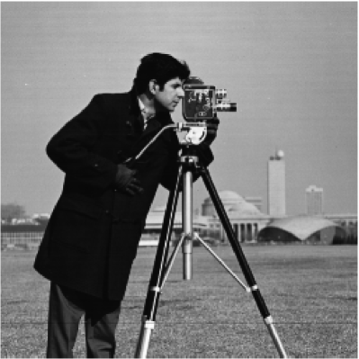
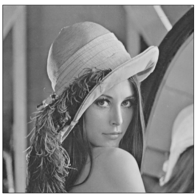
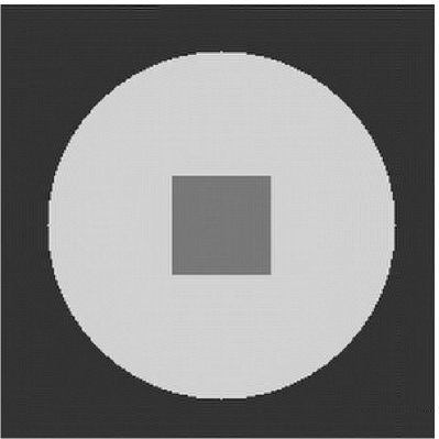
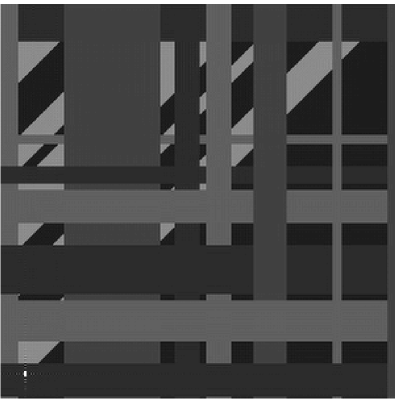
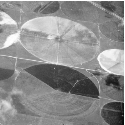
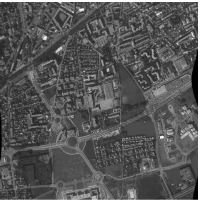
Figure 1: The 7 original images used in the 16 experiments: from top to bottom and left to right: Cameraman, Lena, Sim1, Sim2, Sim3, Fields, and Nîmes.

VI-A Computing the TV Proximity Operator

MIDAL requires, in each iteration, the computation of the TV proximity operator, $\mbox{prox}_{\gamma\phi}$, given by (28), for which we use Chambolle’s fixed point iterative algorithm [8]. Aiming at faster convergence of Chambolle’s algorithm, and consequently of MIDAL, we initialize each run with the dual variables (see [8] for details on the dual variables) computed in the previous run. The underlying rationale is that, as MIDAL proceeds, the images to which the proximity operator is applied get closer; thus, by initializing the computation of the next proximity operator with the internal variables of the previous iteration, the burn-in period is largely avoided.

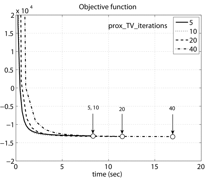
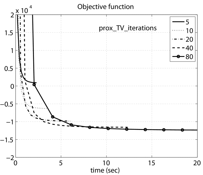
Figure 2: Evolution of the objective function (11) for the setting of Experiment 1, using Chambolle’s fixed point iterative algorithm [8] to compute the TV proximity operator with different initializations. Top plot: initialization with the dual variables computed in the previous iteration. Bottom plot: initialization with the dual variables set to zero.

Another perspective to look at this procedure, already referred to, is given by Theorem 1, which states that there is no need to exactly solve the minimizations in each iteration, but just to ensure the minimization errors along the iterations are absolutely summable. The fulfilment of this condition is easier to achieve with the proposed initialization than with a fixed initialization. Fig. 2 illustrates this aspect. For the setting of Experiment 1, it shows the evolution of the objective function (11) when the dual variables are initialized with the ones computed in the previous iteration (left hand) and when the dual variables are initialized to zero (right hand). All the curves in the top plot reach essentially the same value. Notice that MIDAL takes, approximately, the same time for a number of fixed point iterations between 5 and 20 to compute the TV proximity operator. For a number of iterations higher than 20, MIDAL time increases because, in each iteration, it runs more fixed point iterations than necessary. In the plots in the right hand side, we see that the minimum of the objective function is never reached, although it can be approximated for large values of the fixed point iterations. Based on these observations, we set the number of fixed point iterations to 20 in all experiments of this section.

VI-B Results

Table II reports the results of the 16 experiments. The times for our algorithm and that of [27] are relative to the computer mentioned above. The numbers of iterations are also given, but just as side information since the computational complexity per iteration of each algorithm is different. The initialization of the algorithm of [27] is either the observed image or the mean of the observed image; since the final values of Err are essentially the same for both initializations, we report the best of the two times.

For experiments 8 to 16, we did not have access to the code of [15], so we report the MAE and Err values presented in that paper. According to the authors, their algorithm was run for a fixed number of iterations, thus the computation time depends only on the image size. The time values shown in Table II were provided by the authors and were obtained on a MacBook Pro with a 2.53GHz Intel CoreDuo processor and 4Gb of RAM.

In experiments 1 to 7, our method always achieves lower estimation errors than the method of [27]. Notice that the gain of MIDAL is larger for images with lower SNR, corresponding to the more difficult problems. Moreover, our algorithm is faster than that of [27] in all the experiments, by a factor larger than 3.

In all the experiments 8 to 16, our algorithm achieves lower MAE than the method of [15]. Concerning the relative error Err, our algorithm outperforms theirs in 5 out of 9 cases, there is a tie in two cases, and is outperformed (albeit by a very small margin) in two cases.

TABLE II: Experimental results. Iter, Err, and MAE denote, respectively, the number of iterations, the relative error, and the mean absolute-deviation error. The times are reported in seconds. The time for [15] is referred to a different machine (see text).

	MIDAL				[27]			[15]
Exp.	Err	MAE	Iter	Time	Err	Iter	Time	Err	MAE	Time∗
1	0.130	0.035	21	10	0.151	113	32	–	–	–
2	0.090	0.025	16	8	0.098	115	36	–	–	–
3	0.111	0.036	23	10	0.118	133	38	–	–	–
4	0.069	0.023	17	9	0.071	182	52	–	–	–
5	0.128	0.009	16	1.4	0.143	165	8	–	–	–
6	0.069	0.012	32	21	0.083	166	70	–	–	–
7	0.137	0.023	17	11	0.174	165	69	–	–	–
8	0.089	29.06	61	121	–	–	–	0.096	32.67	245
9	0.066	20.86	34	68	–	–	–	0.066	22.0	245
10	0.056	17.94	29	58	–	–	–	0.055	18.24	245
11	0.301	12.38	25	14	–	–	–	0.314	13.27	245
12	0.217	8.78	25	50	–	–	–	0.217	8.98	245
13	0.170	6.87	23	46	–	–	–	0.174	7.11	245
14	0.167	12.74	33	15	–	–	–	0.192	16.78	54
15	0.124	9.43	19	9	–	–	–	0.131	10.67	54
16	0.097	7.42	56	26	–	–	–	0.091	7.44	54

Figures 3, 4, 5, and 6 show the noisy and restored images, for the Experiments 1 to 4, 5 to 7, 8 to 10, and 11 to 13, respectively. Finally, Fig. 7 plots the evolution of the objective function $L({\bf u}_{k})$ and of the constraint function $\|{\bf z}_{k}-{\bf u}_{k}\|_{2}^{2}$ along the iterations, for the Experiment 1 (Cameraman image and $M=3$). notice the decrease of approximately 7 orders of magnitude of $\|{\bf z}_{k}-{\bf u}_{k}\|_{2}^{2}$ along the 21 MIDAL iterations, showing that, for all practical purposes, the constraint (26) is satisfied.

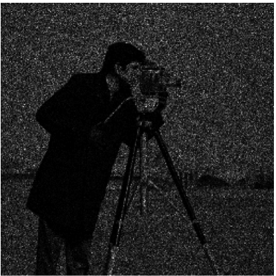
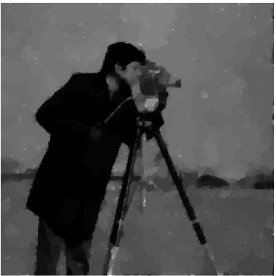
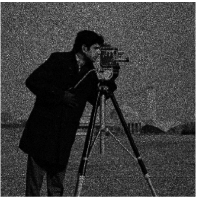
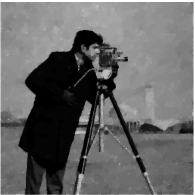
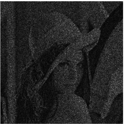
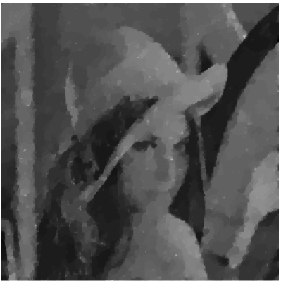
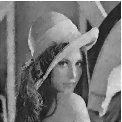
Figure 3: Left column: observed noisy images for Experiments 1 to 4 with $M=3,13,5,33$, respectively. Right column: image estimates.

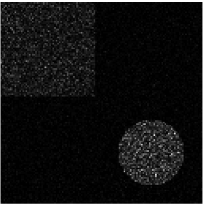
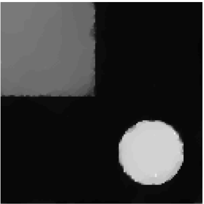
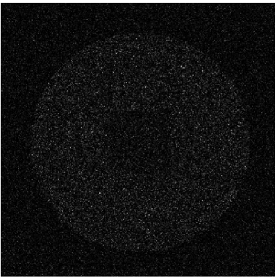
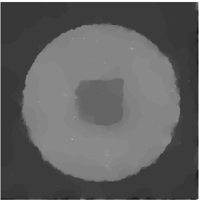
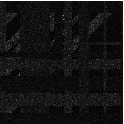
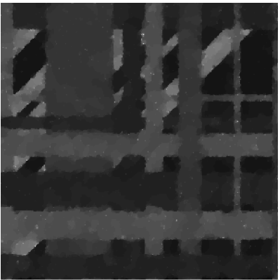
Figure 4: Left column: observed noisy images for Experiments 5 to 7 with $M=2,1,2$, respectively. Right column: image estimates.

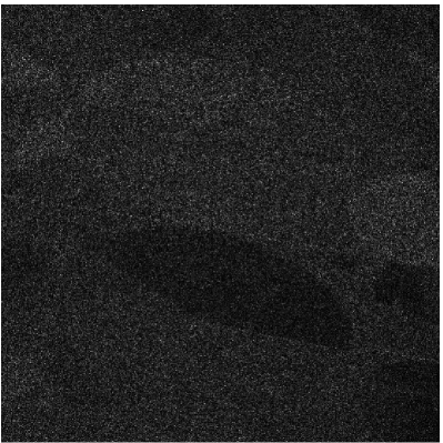
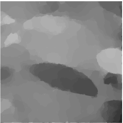
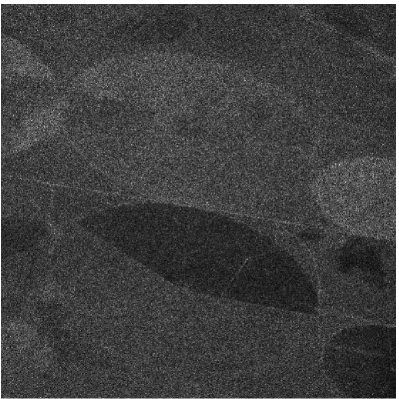
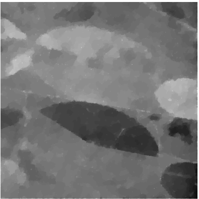
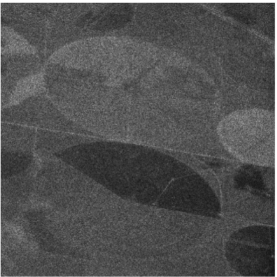
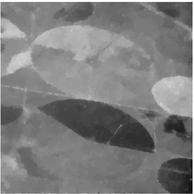
Figure 5: Left column: observed noisy images for Experiments 8 to 10. Right column: image estimates. Note: for better visualization, all the images underwent the nonlinear transformation $(\cdot)^{0.7}$ prior to being displayed.

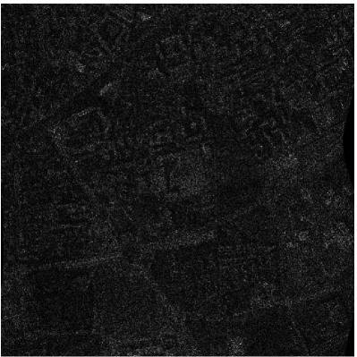
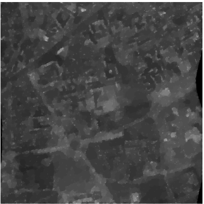
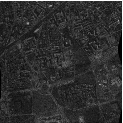
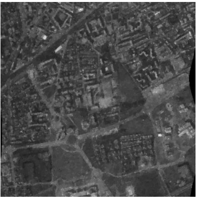
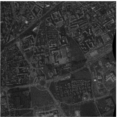
Figure 6: Left column: observed noisy images for Experiments 11 to 13. Right column: image estimates. Note: for better visualization, all the images underwent the nonlinear transformation $(\cdot)^{0.7}$ prior to being displayed.

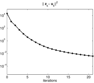
Figure 7: Evolution of the objective function $L({\bf u}_{k})$ and of the constraint function $\|{\bf z}_{k}-{\bf u}_{k}\|_{2}^{2}$, along the iterations of the algorithm, for Experiment 1.

VII Concluding Remarks

We have proposed a new approach to solve the optimization problem resulting from variational (equivalently MAP) estimation of images observed under multiplicative noise models. Although the proposed formulation and algorithm can be used with other priors (namely, frame-based), here we have focused on total-variation regularization. Our approach is based on two building blocks: (1) the original unconstrained optimization problem was first transformed into an equivalent constrained problem, via a variable splitting procedure; (2) this constrained problem was then addressed using an augmented Lagrangian method, more specifically, the alternating direction method of multipliers (ADMM). We have shown that the conditions for the convergence of ADMM are satisfied.

Multiplicative noise removal (equivalently reflectance estimation) was formulated with respect to the logarithm of the reflectance, as proposed by some other authors. As a consequence, the multiplicative noise was converted into additive noise yielding a strictly convex data term (i.e., negative of the log-likelihood function), which was not the case with the original multiplicative noise model. A consequence of this strict convexity, together with the convexity of the total variation regularizer, was that the solution of the variational problem (the denoised image) is unique and the resulting algorithm, termed MIDAL (multiplicative image denoising by augmented Lagrangian), is guaranteed to converge.

MIDAL is very simple and, in the experiments herein reported, exhibited state-of-the-art estimation performance and speed. For example, compared with the hybrid method in [15], which combines curvelet-based and total-variation regularization, MIDAL yields comparable or better results in all the experiments.

We are currently working on extending our approach to problems involving linear observation operators (e.g., blurs), other non-additive and non-Gaussian noise models, such as Poissonian observations [19], [36], and other regularizers, such as those based on frame representations.

References

- [1] G. Aubert and J. Aujol, “A variational approach to remove multiplicative noise”, SIAM Journal of Applied Mathematics, vol. 68, no. 4, pp. 925–946, 2008.
- [2] M. Bazaraa, H. Sherali, and C. Shetty, Nonlinear Programming: Theory and Algorithms, John Wiley & Sons, New York, 1993.
- [3] A. Beck and M. Teboulle, “A fast iterative shrinkage-thresholding algorithm for linear inverse problems”, SIAM Journal on Imaging Sciences, vol. 2, pp. 183 202, 2009.
- [4] J. Bioucas-Dias and M. Figueiredo, “An iterative algorithm for linear inverse problems with compound regularizers”, Proceedings of the IEEE International Conference on Image Processing - ICIP’2008, San Diego, CA, USA, 2008.
- [5] J. Bioucas-Dias and M. Figueiredo, “Total variation restoration of speckled images using a split-Bregman algorithm”, Proceedings of the IEEE International Conference on Image Processing - ICIP’2009, Cairo, Egypt, 2009.
- [6] J. Bioucas-Dias and M. Figueiredo, “A new TwIST: two-step iterative shrinkage/thresholding algorithms for image restoration”, IEEE Transactions on Image Processing, vol. 16, pp. 2980-2991, 2007.
- [7] J. Bioucas-Dias, T. Silva, and J. Leitão, “Adaptive restoration of speckled SAR images”, Proceedings of the IEEE International Geoscience and Remote Sensing Symposium – GRSS’98, vol. I, pp. 19–23, 1998.
- [8] A. Chambolle, “An algorithm for total variation minimization and applications,” Journal of Mathematical Imaging and Vision, vol. 20, pp. 89-97, 2004.
- [9] T. Chan, S. Esedoglu, F. Park, and A. Yip, “Recent developments in total variation image restoration,” in Mathematical Models of Computer Vision, Springer, 2005.
- [10] T. Chan, G. Golub, and P. Mulet, “A nonlinear primal-dual method for total variation-based image restoration”, SIAM Journal on Scientific Computing, vol. 20, pp. 1964–1977, 1999.
- [11] C. Chesneau, J. Fadili, and J.-L. Starck, “Stein block thresholding for image denoising”, Applied and Computational Harmonic Analysis, vol. 28, pp. 67- 88, 2010.
- [12] P. L. Combettes and J.-C. Pesquet, “A Douglas-Rachford splitting approach to nonsmooth convex variational signal recovery,” IEEE Journal of Selected Topics in Signal Processing, vol. 1, pp. 564-574, 2007.
- [13] P. L. Combettes and V. Wajs, “Signal recovery by proximal forward-backward splitting,” SIAM Journal on Multiscale Modeling & Simulation, vol. 4, pp. 1168–1200, 2005.
- [14] R. Corless, G. Gonnet, D. Hare, D. Jeffrey, and D. Knuth, “On the Lambert W function”, Advances in Computational Mathematics, vol. 5, pp. 329–359, 1996.
- [15] S. Durand, J. Fadili, and M. Nikolova, “Multiplicative noise removal using L1 fidelity on frame coefficients”, Journal of Mathematical Imaging and Vision, 2009 (to appear).
- [16] J. Eckstein and D. Bertsekas, “On the Douglas Rachford splitting method and the proximal point algorithm for maximal monotone operators”, Mathematical Programming, vol. 5, pp. 293 -318, 1992.
- [17] E. Esser, “Applications of Lagrangian-based alternating direction methods and connections to split Bregman”, Technical Report 09-31, Computational and Applied Mathematics, University of California, Los Angeles, 2009.
- [18] M. Figueiredo, J. Bioucas-Dias, J. Oliveira, and R. Nowak, “On total-variation denoising: A new majorization-minimization algorithm and an experimental comparison with wavalet denoising,” Proceedings of the IEEE International Conference on Image Processing – ICIP’06, 2006.
- [19] M. Figueiredo and J. Bioucas-Dias, “Deconvolution of Poissonian images using variable splitting and augmented Lagrangian optimization”, Proceedings of the IEEE Workshop on Statistical Signal Processing – SSP 2009, Cardiff, 2009. Available at http://arxiv.org/abs/0904.4868
- [20] V. Frost, K. Shanmugan, and J. Holtzman, “A model for radar images and its applications to adaptive digital filtering of multiplicative noise”, IEEE Transactions on Pattern Analysis and Machine Intelligence, vol. 2, pp. 157–166, 1982.
- [21] D. Gabay and B. Mercier, “A dual algorithm for the solution of nonlinear variational problems via finite-element approximations”, Computers and Mathematics with Applications, vol. 2, pp. 17–40, 1976.
- [22] R. Glowinski and A. Marroco, “Sur l’approximation, par elements finis d’ordre un, et la resolution, par penalisation-dualité d’une classe de problemes de Dirichlet non lineares”, Revue Française d’Automatique, Informatique et Recherche Opérationelle, vol. 9, pp. 41–76, 1975.
- [23] T. Goldstein and S. Osher, “The split Bregman method for L1 regularized problems”, SIAM Journal on Imaging Science, vol. 2, pp. 323–343, 2009.
- [24] J. Goodman, “Some fundamental properties of speckle”, Journal of the Optical Society of America, vol. 66, pp. 1145–1150, 1976.
- [25] J. Goodman, Speckle Phenomena in Optics: Theory and Applications, Roberts and Company Publishers, 2007.
- [26] M. Hestenes, “Multiplier and Gradient Methods”, Journal of Optimization Theory and Applications, vol. 4, pp. 303-320, 1969.
- [27] Y. Huang, M. Ng, and Y. Wen, “A new total variation method for multiplicative noise removal”, SIAM Journal on Imaging Sciences, vol. 2, no. 1, pp. 20–40, 2009.
- [28] A. Iusem, “Augmented Lagrangian methods and proximal point methods for convex optimization”, Investigación Operativa, vol. 8, pp. 11–49, 1999.
- [29] C. Jakowatz, D. Wahl, P. Eichel, D. Ghiglia, and P. Thompson, Spotlight-Mode Synthetic Aperture Radar: A Signal Processing Approach, Kluwer Academic Publishers, 1996.
- [30] J. Nocedal and S. Wright, Numerical Optimization, Springer, 2006.
- [31] C. Oliver and S. Quegan, Understanding Synthetic Aperture Radar Images, Artech House, 1998.
- [32] S. Osher, L. Rudin, and E. Fatemi, “Nonlinear total variation based noise removal algorithms,” Physica D, vol. 60, pp. 259–268, 1992.
- [33] M. Powell, “A Method for nonlinear Constraints in Minimization Problems”, in Optimization, R. Fletcher, (editor), Academic Press, pp. 283–298, New York, 1969.
- [34] L. Rudin, P. Lions, and S. Osher, “Multiplicative denoising and deblurring: theory and algorithms”, in Geometric Level Set Methods in Imaging, Vision, and Graphics, S. Osher and N. Paragios (editors), pp. 103–120, Springer, 2003.
- [35] S. Setzer, “Split Bregman algorithm, Douglas-Rachford splitting, and frame shrinkage”, Proceedings of the Second International Conference on Scale Space Methods and Variational Methods in Computer Vision, LNCS vol. 5567, pp. 464-476, Springer, 2009.
- [36] S. Setzer, G. Steidl and T. Teuber, “Deblurring Poissonian images by split Bregman techniques”, Journal of Visual Communication and Image Representation, 2009 (to appear).
- [37] J. Shi and S. Osher, “A nonlinear inverse scale space method for a convex multiplicative noise model”, Technical Report 07-10, Computational and Applied Mathematics, University of California, Los Angeles, 2007.
- [38] G. Steidl and T. Teuber, “Removing multiplicative noise by Douglas-Rachford splitting methods”, Journal of Mathematical Imaging and Vision, 2009 (to appear).
- [39] X. Tai and C. Wu, “Augmented Lagrangian method, dual methods and split Bregman iteration for ROF model”, Technical Report 09-05, Computational and Applied Mathematics, University of California, Los Angeles, 2009.
- [40] Y. Wang, J. Yang, W. Yin, and Y. Zhang, “A new alternating minimization algorithm for total variation image reconstruction”, SIAM Journal on Imaging Sciences, vol. 1, no. 3, pp. 248–272, 2008.
- [41] S. Wright, R. Nowak, M. Figueiredo, “Sparse reconstruction by separable approximation , IEEE Transactions on Signal Processing, vol. 57, pp. 2479-2493, 2009.
- [42] W. Yin, S. Osher, D. Goldfarb, J. Darbon, “Bregman iterative algorithms for -minimization with applications to compressed sensing”, SIAM Journal on Imaging Sciences, vol. 1, no. 1, pp. 143–168, 2008.
- [43] M. Zhu, S. Wright, and T. Chan, “Duality-based algorithms for total variation image restoration”, Technical Report 08-33, Computational and Applied Mathematics, University of California, Los Angeles, 2008.