Local Asymptotics of $P$-Spline Smoothing

Abstract

This paper addresses asymptotic properties of general penalized spline estimators with an arbitrary B-spline degree and an arbitrary order difference penalty. The estimator is approximated by a solution of a linear differential equation subject to suitable boundary conditions. It is shown that, in certain sense, the penalized smoothing corresponds approximately to smoothing by the kernel method. The equivalent kernels for both inner points and boundary points are obtained with the help of Green’s functions of the differential equation. Further, the asymptotic normality is established for the estimator at interior points. It is shown that the convergence rate is independent of the degree of the splines, and the number of knots does not affect the asymptotic distribution, provided that it tends to infinity fast enough.

Key Words: Difference penalty, equivalent kernel, Green’s function, $P$-spline.

1 Introduction

Consider the problem of estimating the function $f:\mathbb{[}0,1]\rightarrow\mathbb{R}$ from a univariate regression model $y_{i}=f(t_{i})+\epsilon_{i}$, $i=1,\ldots,n$, where the $t_{i}$ are pre-specified design points and the $\epsilon_{i}$ are iid normal random variables with mean $0$ and variance $\sigma^{2}$. This paper presents a local asymptotic theory of penalized spline estimators of $f$.

The penalized spline regression model with difference penalty was introduced by Eilers and Marx (1996), who coined the term “$P$-splines”, but using less knots for the regression problem can be traced back at least to O’Sullivan (1986). Penalized spline smoothing has become popular over the last decade and the uses of low rank bases lead to highly tractable computation. The methodology and applications of $P$-splines are discussed extensively in Ruppert, Wand and Carroll (2003). On the other hand, asymptotic properties of the $P$-spline estimators are less explored in the literature. A few exceptions include recent papers such as Hall and Opsomer (2005), Li and Ruppert (2008), and Claeskens, Krivobokova, and Opsomer (2009). Hall and Opsomer (2005) placed knots continuously over a design set and established consistency of the estimator. Li and Ruppert (2008) developed an asymptotic theory of $P$-splines for piecewise constant and linear B-splines with the first and second order difference penalties. Claeskens, Krivobokova, and Opsomer (2009) studied bias, variance and asymptotic rates of the $P$-spline estimator under different choices of the number of knots and penalty parameters. An interested reader may also refer to Pal and Woodroofe (2007), Shen and Wang (2009), and Wang and Shen (2009) for shape constrained regression estimators and their applications.

The $P$-spline model approximates the regression function by $f^{[p]}(x)=\sum_{k=1}^{K_{n}+p}b_{k}B^{[p]}_{k}(x)$, where $\big{\{}B^{[p]}_{k}:k=1,\ldots,K_{n}+p\,\big{\}}$ is the $p\,$th degree B-spline basis with knots $0=\kappa_{0}<\kappa_{1}<\cdots<\kappa_{K_{n}}=1$. The value of $K_{n}$ will depend upon $n$ as discussed below. The spline coefficients $\hat{b}=\{\hat{b}_{k},k=1,\ldots,K_{n}+p\}$ subject to the $m$th-order difference penalty are chosen to minimize

$$\sum_{i=1}^{n}\big{[}y_{i}-\sum_{k=1}^{K_{n}+p}b_{k}B_{k}^{[p]}(t_{i})\big{]}^{2}+\lambda^{*}\sum_{k=m+1}^{K_{n}+p}\big{[}\Delta^{m}(b_{k})\big{]}^{2},$$ (1)

where $\lambda^{*}>0$ and $\Delta$ is the backward difference operator, i.e., $\Delta b_{k}\equiv b_{k}-b_{k-1}$ and

$$\Delta^{m}b_{k}=\Delta\Delta^{m-1}b_{k}=\cdots=\sum_{j=0}^{m}(-1)^{m-j}{m\choose j}b_{k-m+j}.$$ (2)

For simplicity, we assume that both the design points and the knots are equally spaced on the interval $[0,1]$. We also assume that $n/K_{n}$ is an integer denoted by $M_{n}$. Hence every $M_{n}$th design point is a knot, that is, $\kappa_{j}=t_{jM_{n}}$ for $j=1,\ldots,K_{n}$; a more general case is discussed briefly in Section 6. The $P$-spline estimator is given by $\hat{f}^{[p]}(x)=\sum_{k=1}^{K_{n}+p}\hat{b}_{k}B^{[p]}_{k}(x)$.

This paper develops a general asymptotic theory of $P$-splines under an arbitrary choice of $p$ and $m$. It is shown that the $P$-spline estimator can be approximated by the solution of an ordinary differential equation (ODE) with suitable boundary conditions. This estimator is then shown to be described by a kernel estimator, using a Green’s function obtained from a closely related boundary value problem as a kernel. The asymptotic properties of the estimator thus are explicitly established based on the Green’s function and the solution of the differential equation. It is worth mentioning that asymptotic analysis of smoothing splines using Green’s functions was performed by Rice and Rosenblatt (1983), Silverman (1984), Messer (1991), Nychka (1995) and Pal and Woodroofe (2007). However, these papers only treat limited special cases. In contrast, the current paper develops a general framework for $P$-splines. This framework leads to a relatively simpler approach to obtain a closed-form expression of an equivalent kernel for both inner points and boundary points at the first time. Further, we show that the convergence rate of $\hat{f}^{[p]}$ depends only on $m$ but not on $p$, as long as $K_{n}$ tends to infinity fast enough; see Corollary 4.1 where $K_{n}$ is of order $n^{\gamma}$, where $\gamma>(2m-1)/(4m+1)$.

The contributions of the present paper are twofold: (i) the paper develops a general approach for asymptotic analysis of a $P$-spline estimator with an arbitrary spline degree and arbitrary order difference penalty via Green’s functions. To handle a general $P$-spline estimator, various techniques for linear ODEs are exploited to obtain a corresponding Green’s function. (ii) the closed-form expressions of equivalent kernels for both inner and boundary points are established and convergence rates are developed for general $P$-spline estimators. Compared with the existing results based on matrix techniques, e.g. Li and Ruppert (2008) and Claeskens, Krivobokova, and Opsomer (2009), the use of Green’s functions considerably simplifies the development and yields an instrumental alternative to establish the equivalent kernels for general $P$-splines. Moreover, this also leads to the convergence rates and the observation that the rates are independent of the splines’ degrees and the number of knots for an arbitrary $P$-spline estimator. While this observation is pointed out by Li and Ruppert (2008) for piecewise constant and piecewise linear splines and is conjectured for general $P$-splines, no rigorous justification has been given for general $P$-splines in the literature; the current paper offers a satisfactory answer to this issue in a general setting.

The paper is organized as follows. Section 2 characterizes the general $P$-spline estimator as an approximate solution of a linear differential equation subject to suitable boundary conditions. Section 3 investigates the solution of such the differential equation and obtains the related Green’s functions as equivalent kernels for a $P$-spline estimator of an arbitrary B-spline degree with any order difference penalty. Using these Green’s functions, the asymptotic properties of $P$-splines are established in Section 4. Section 5 addresses kernel approximation near the boundary of the design set. By formulating boundary conditions as an appropriate integral form, an explicit equivalent kernel is obtained. Finally, extensions to unequally spaced data and multivariate $P$-splines are discussed in Section 6.

2 Characterization of the estimator

Let $X=[B_{k}(x_{i})]\in\mathbb{R}^{n\times(K_{n}+p)}$ be the design matrix, and let $D_{m}\in\mathbb{R}^{(K+p-m)\times(K+p)}$ be the $m$th-order difference matrix such that $D_{m}b=[\Delta^{m}(b_{m+1}),\ldots,\Delta^{m}(b_{K_{n}+p})]^{T}$. The optimality condition is given by

$$(X^{T}X+\lambda^{*}D_{m}^{T}D_{m})\hat{b}=X^{T}y,$$ (3)

where $y=(y_{1},\ldots,y_{n})^{T}$.

To characterize the $P$-spline estimator $\hat{f}^{[p]}$, we introduce more notation. Define $C\in\mathbb{R}^{(K_{n}+p)\times(K_{n}+p)}$ and $\tilde{C}\in\mathbb{R}^{(K_{n}+p)\times n}$, respectively, as

$$C=\left[\begin{array}[]{ccccccccc}1&0&0&0&\cdots&0&0\\ 1&1&0&0&\cdots&0&0\\ 1&1&1&0&\cdots&0&0\\ &\cdots&&&\cdots&&\\ 1&1&1&1&\cdots&1&0\\ 1&1&1&1&\cdots&1&1\end{array}\right]~{}~{}~{}\mbox{and}~{}~{}~{}\tilde{C}=\left[\begin{array}[]{cccccccccccccccccc}0&0&0&\cdots&0&0\\ &\cdots&&\cdots&&\\ 0&0&0&\cdots&0&0\\ {\bf 1}^{T}&0&0&\cdots&0&0\\ {\bf 1}^{T}&{\bf 1}^{T}&0&\cdots&0&0\\ &\cdots&&\cdots&&\\ {\bf 1}^{T}&{\bf 1}^{T}&{\bf 1}^{T}&\cdots&{\bf 1}^{T}&0\\ {\bf 1}^{T}&{\bf 1}^{T}&{\bf 1}^{T}&\cdots&{\bf 1}^{T}&{\bf 1}^{T}\end{array}\right],$$

where ${\bf 1}=[1,1,\cdots,1]^{T}\in\mathbb{R}^{M_{n}\times 1}$. Since $C$ is invertible, for any $k\in\mathbb{N}$, (3) is equivalent to

$$\lambda^{*}C^{k}D_{m}^{T}D_{m}\hat{b}+C^{k}X^{T}\hat{f}=C^{k}X^{T}y,$$ (4)

where $\hat{f}=[\hat{f}^{[p]}(x_{1}),\ldots,\hat{f}^{[p]}(x_{n})]^{T}$ and $C^{k}=\underbrace{CC\cdots C}_{k-\mbox{copies}}$. The matrix $D_{m}^{T}D_{m}$ is a banded symmetric matrix. Except for the first $m$ and last $m$ rows, every row of $D_{m}^{T}D_{m}$ has the form $(0,\cdots,0,\omega_{0}^{*},\omega_{1}^{*},\cdots,\omega_{2m}^{*},0,\cdots,0)$, where $\omega_{j}^{*}=(-1)^{m}(-1)^{2m-j}{2m\choose j}$, $j=0,\ldots,2m$. Moreover, except for the first $m-k$ and last $m$ rows, the $i$th row of $C^{k}D_{m}^{T}D_{m}$ has the form

$$\Big{(}\,\underbrace{0,\cdots,0,}_{(i-m+k-1)-\mbox{copies}}\omega_{0},\cdots,\omega_{2m-k},\underbrace{0,\cdots,0}_{(K_{n}+p)-(i+m)-\mbox{copies}}\,\Big{)},$$

where

$$\omega_{j}=(-1)^{m}(-1)^{2m-k-j}{2m-k\choose j},\ j=0,\ldots,2m-k.$$ (5)

Further, the elements of the last $k$ rows of $C^{k}D_{m}^{T}D_{m}$ are all zeros. In particular, when $k=m$,

$$C^{m}D_{m}^{T}D_{m}\hat{b}=(-1)^{m}\ \big{[}~{}\Delta^{m}\hat{b}_{m+1},\Delta^{m}\hat{b}_{m+2},\cdots,\Delta^{m}\hat{b}_{K_{n}+p},0,\ldots,0~{}\big{]}^{T}.$$ (6)

It is also interesting to note the derivative formula for B-spline functions (de Boor, 2001)

$${d^{\,l}\over dx^{l}}\sum_{k=1}^{K_{n}+p}b_{k}B_{k}^{[p]}(x)=\sum_{k=l+1}^{K_{n}+p}K_{n}^{l}\Delta^{l}b_{k}\ B_{k-1}^{[p-l]}(x),~{}~{}~{}l\leq p.$$ (7)

Hence,

$${d^{m}\over dx^{m}}\sum_{k=1}^{K_{n}+m}\hat{b}_{k}B_{k}^{[m]}(x)=K_{n}^{m}\sum_{k=m+1}^{K_{n}+m}\Delta^{m}\hat{b}_{k}B_{k-m}^{[0]}(x),$$

and therefore,

$$\Delta^{m}\hat{b}_{m+k}={1\over K_{n}^{m}}{d^{m}\over dx^{m}}\hat{f}^{[m]}(x),~{}~{}~{}~{}x\in(\kappa_{k-1},\kappa_{k}],~{}~{}~{}k=1,\ldots,K_{n}.$$ (8)

Let $\omega_{1}$ be the uniform distribution on $x_{1},\ldots,x_{n}$ and $\omega_{2}$ be the uniform distribution on $\kappa_{1},\ldots,\kappa_{K_{n}}$. Let $g$ and $\check{f}$ be two piecewise constant functions for which $g(x_{k})=y_{k}$ and $\check{f}(x_{k})=\hat{f}(x_{k})$ for $k=1,...,n$, respectively. Let $G_{1}(x)=\int_{0}^{x}g(t)d\omega_{1}(t)$, $\check{F}_{1}(x)=\int_{0}^{x}\check{f}(t)d\omega_{1}(t)$, $\hat{F}_{1}(x)=\int_{0}^{x}\hat{f}(t)dt$, and for $k\geq 2$, define

$$G_{k}(x)=\int_{0}^{x}G_{k-1}(t)d\omega_{2}(t),~{}~{}~{}~{}\check{F}_{k}(x)=\int_{0}^{x}\check{F}_{k-1}(t)d\omega_{2}(t),~{}~{}~{}~{}\hat{F}_{k}(x)=\int_{0}^{x}\hat{F}_{k-1}(t)dt.$$

To obtain the analogous representation for $\hat{f}$, we introduce a few variables and functions related to the true regression function $f$. Define $\Phi_{1}(x)=\int_{0}^{x}f(t)dt$, $\tilde{\Phi}_{1}(x)=\int_{0}^{x}f(t)d\omega_{1}(t)$, and for $k\geq 2$,

$$\Phi_{k}(x)=\int_{0}^{x}\Phi_{k-1}(t)dt,~{}~{}~{}~{}\tilde{\Phi}_{k}(x)=\int_{0}^{x}\tilde{\Phi}_{k-1}(t)d\omega_{2}(t).$$

Letting $R=C\ X^{T}-\tilde{C}$, we have $C^{m}X^{T}\hat{f}=C^{m-1}\tilde{C}\hat{f}+C^{m-1}R\hat{f}$. Therefore, the $j$th row of (4), when $k=m$, can be written as

$$\check{F}_{m}(\kappa_{j+p-1})+R_{fj}+(-1)^{m}{\lambda^{*}\over nK_{n}^{m-1}}\Delta^{m}b_{m+j}=G_{m}(\kappa_{j+p-1})+R_{yj},\ \ j=1,\ldots,K_{n},$$ (9)

where $R_{fj}$ and $R_{yj}$ are the $j$th row of ${1\over nK_{n}^{m-1}}C^{m-1}R\hat{f}$ and ${1\over nK_{n}^{m-1}}C^{m-1}Ry$, respectively. Furthermore, since the elements of the last $k$ rows of $C^{k}D_{m}^{T}D_{m}$ are all zeros, we also have

$$\check{F}_{k}(1)=G_{k}(1),~{}~{}~{}~{}~{}k=1,\ldots,m.$$ (10)

Next, we proceed by replacing that difference equation (9) by an analogous differential equation. We shall focus on the case when $p=m$ first; the case when $p\neq m$ will be discussed in Section 4. For any $x\in[0,1]$, letting $k_{x}=\lfloor K_{n}x\rfloor+1$, (9) gives

$$\check{F}_{m}(\kappa_{k_{x}+p})+R_{f,k_{x}+1}+(-1)^{m}{\lambda^{*}\over nK_{n}^{m-1}}\Delta^{m}b_{m+k_{x}+1}=G_{m}(\kappa_{k_{x}+p})+R_{y,k_{x}+1}.$$ (11)

Define

$$\tilde{R}(x)=\hat{F}_{m}(x)-G_{m}(x)+G_{m}(\kappa_{k_{x}+p})-\check{F}_{m}(\kappa_{k_{x}+p})+R_{y,k_{x}+1}-R_{f,k_{x}+1}.$$ (12)

Then, from (8) and (11), $\hat{F}_{m}$ solves the ordinary differential equation

$$(-1)^{m}\alpha\hat{F}^{(2m)}_{m}(x)+\hat{F}_{m}(x)=G_{m}(x)+\tilde{R}(x),~{}~{}~{}~{}0\leq x\leq 1,$$ (13)

where $\alpha=\lambda^{*}/(nK_{n}^{2m-1})$. We have $2m$ boundary conditions for (13):

$$\hat{F}_{m}^{(k)}(0)=0,~{}~{}~{}\hat{F}_{m}^{(k)}(1)=G_{m-k}(1)+e_{m-k},~{}~{}~{}k=0,\ldots,m-1,$$

where $e_{m-k}=\hat{F}_{m}^{(k)}(1)-\check{F}_{m-k}(1)$. We shall show that $\hat{f}^{[p]}$ is stochastically bounded, therefore the $e_{k}$ are small with an order of $O_{p}(1/n)$.

3 Green’s functions

The solution to (13) can be represented by a corresponding Green’s function explicitly. It shall be shown that the $P$-spline estimator can be approximated by a kernel estimator, using the corresponding Green’s function. For this end, consider the differential equation

$$(-1)^{m}\alpha F^{(2m)}(t)+F(t)=G(t),~{}~{}~{}~{}~{}~{}~{}0\leq t\leq 1,$$ (14)

subject to the boundary conditions $F^{(i)}(0)=0$ and $F^{(i)}(1)=G^{(i)}(1)$, $i=0,\ldots,m-1$. Let $\beta\equiv\alpha^{-1/(2m)}$. We consider two cases: (1) $m$ is even; and (2) $m$ is odd.

3.1 Even $m$

In this case, the characteristic equation is given by $\lambda^{2m}+\beta^{2m}=0$, and we obtain $2m$ eigenvalues

$$\lambda_{k}=\beta\Big{[}\cos\frac{(1+2k)\pi}{2m}+\imath\,\sin\frac{(1+2k)\pi}{2m}\Big{]},\ \ \ k=0,1,\cdots,2m-1.$$

Let

$$\mu_{k}=\cos\frac{(1+2k)\pi}{2m}~{}~{}\mbox{ and }~{}~{}\omega_{k}=\sin\frac{(1+2k)\pi}{2m}.$$

Then the homogeneous ODE: $\alpha F^{(2m)}(t)+F(t)=0$ has $2m$ solutions

$$e^{(\pm\mu_{k}\pm\imath\omega_{k})\beta t}=e^{\pm\beta\mu_{k}t}\,\big{[}\cos(\beta\omega_{k}t)\pm\imath\,\sin(\beta\omega_{k}t)\big{]},\ \ \ k=0,\cdots,\frac{m}{2}-1,$$

where $\mu_{k}>0$ and $\omega_{k}>0$ for $k=0,\cdots,\frac{m}{2}-1$.

To find the corresponding Green’s function for the ODE: $\alpha F^{(2m)}(t)+F(t)=G(t)$ on $[0,1]$, we define the following function

$$L(t)\,\equiv\,\sum^{\frac{m}{2}-1}_{k=0}\,\beta\,e^{-\beta\mu_{k}t}\big{[}\,c_{k}\,\cos(\omega_{k}\beta t)+d_{k}\,\sin(\omega_{k}\beta t)\big{]},$$ (15)

where the coefficients $c_{k},d_{k}$ are to be determined, and $K(t,s)\,\equiv\,L(|t-s|).$ Since $L$ is a linear combination of the solutions of the homogeneous ODE, $L^{(2m)}+\beta^{2m}L=0$ also holds. Let

$$F_{0}(t)\equiv\int^{1}_{0}K(t,s)G(s)ds,\ \ \ t\in[0,1].$$

By noting $F_{0}(t)=\int^{t}_{0}L(t-s)G(s)ds+\int^{1}_{t}L(s-t)G(s)ds$ for all $t\in[0,1]$, it is easy to verify that if

$$L^{(k)}(t)\big{|}_{t=0}=0,\ \ \forall\ \ k=1,3,\cdots,2m-3,\ \ \mbox{ and }\ \ \ L^{(2m-1)}(t)\big{|}_{t=0}=\frac{\beta^{\,2m}}{2},$$ (16)

then $F_{0}(t)$ is a solution of $\alpha F^{(2m)}+F=G$.

To find the coefficients $c_{k},d_{k}$, define

$$p_{\,k}(t)\,\equiv\,e^{-\beta\mu_{k}t}\big{[}\,c_{k}\,\cos(\omega_{k}\beta t)+d_{k}\,\sin(\omega_{k}\beta t)\big{]},\ \ \ q_{k}(t)\,\equiv\,e^{-\beta\mu_{k}t}\big{[}\,-c_{k}\,\sin(\omega_{k}\beta t)+d_{k}\,\cos(\omega_{k}\beta t)\big{]}.$$

Hence $p_{\,k}(0)=c_{k}$ and $q_{k}(0)=d_{k}$. Since

$$\begin{pmatrix}p^{\prime}_{\,k}(t)\\ q^{\prime}_{k}(t)\end{pmatrix}\,=\,\beta\underbrace{\begin{bmatrix}-\mu_{k}&\omega_{k}\\ -\omega_{k}&-\mu_{k}\end{bmatrix}}_{A_{k}}\begin{pmatrix}p_{\,k}(t)\\ q_{k}(t)\end{pmatrix},$$ (17)

we have

$$\begin{pmatrix}p^{(j)}_{\,k}(t)\\ q^{(j)}_{k}(t)\end{pmatrix}\,=\,\big{(}\beta A_{k}\big{)}^{j}\begin{pmatrix}p_{\,k}(t)\\ q_{k}(t)\end{pmatrix},$$

where $p^{(j)}_{\,k}(t)$ and $q^{(j)}_{k}(t)$ stand for the $j$-th derivatives of $p_{k}$ and $q_{k}$ respectively. Letting $A^{j}_{k}(i,\ell)$ denote the $(i,\ell)$-element of $A^{j}_{k}$, we obtain the following linear equation for $\{c_{k},d_{k}\}$ from (16):

$${\small\underbrace{\begin{bmatrix}A_{0}(1,1)&A_{0}(1,2)&\cdots&\cdots&A_{\frac{m}{2}-1}(1,1)&A_{\frac{m}{2}-1}(1,2)\\ A^{3}_{0}(1,1)&A^{3}_{0}(1,2)&\cdots&\cdots&A^{3}_{\frac{m}{2}-1}(1,1)&A^{3}_{\frac{m}{2}-1}(1,2)\\ \vdots&\vdots&&&\vdots&\vdots\\ A^{(2m-3)}_{0}(1,1)&A^{(2m-3)}_{0}(1,2)&\cdots&\cdots&A^{(2m-3)}_{\frac{m}{2}-1}(1,1)&A^{(2m-3)}_{\frac{m}{2}-1}(1,2)\\ A^{(2m-1)}_{0}(1,1)&A^{(2m-1)}_{0}(1,2)&\cdots&\cdots&A^{(2m-1)}_{\frac{m}{2}-1}(1,1)&A^{(2m-1)}_{\frac{m}{2}-1}(1,2)\end{bmatrix}}_{A^{e}}\begin{bmatrix}c_{0}\\ d_{0}\\ \vdots\\ c_{\frac{m}{2}-1}\\ d_{\frac{m}{2}-1}\end{bmatrix}\,=\,\begin{bmatrix}0\\ 0\\ \vdots\\ 0\\ \frac{1}{2}\end{bmatrix}.}$$ (18)

It shall be shown in Lemma 3.1 that the above equation has a unique solution.

3.2 Odd $m$

The characteristic equation is given by $\lambda^{2m}-\beta^{2m}=0$ and the eigenvalues are:

$$\lambda_{k}=\beta\Big{(}\cos\frac{k\pi}{m}+\imath\,\sin\frac{k\pi}{m}\Big{)},\ \ \ k=0,1,\cdots,2m-1.$$

Then the homogeneous ODE: $\alpha F^{(2m)}(t)+F(t)=0$ has $2m$ solutions: $e^{\pm\beta t}$ and

$$e^{(\pm\mu_{k}\pm\imath\omega_{k})\beta t}=e^{\pm\beta\mu_{k}t}\,\big{[}\cos(\beta\omega_{k}t)\pm\imath\,\sin(\beta\omega_{k}t)\big{]},\ \ \ k=1,\cdots,\frac{m-1}{2},$$

where $\mu_{k}=\cos\frac{k\pi}{m}>0$ and $\omega_{k}=\sin\frac{k\pi}{m}>0$ for $k=1,\cdots,\frac{m-1}{2}$. Similar to the even case, define

$$P(t)\,\equiv\,c_{0}\,\beta e^{-\beta t}+\sum^{(m-1)/2}_{k=1}\,\beta\,e^{-\beta\mu_{k}t}\big{[}\,c_{k}\,\cos(\omega_{k}\beta t)+d_{k}\,\sin(\omega_{k}\beta t)\big{]},$$ (19)

where the coefficients $c_{k},d_{k}$ are to be determined, and $P(t)$ satisfies $P^{(2m)}(t)-\beta^{2m}P(t)=0$. Let $K(t,s)\equiv P(|t-s|)$ and $F_{0}(t)\equiv\int^{1}_{0}K(t,s)G(s)ds$. It can be verified that if

$$P^{(k)}(t)\big{|}_{t=0}=0,\ \ \forall\ \ k=1,3,\cdots,2m-3,\ \ \mbox{ and }\ \ \ P^{(2m-1)}(t)\big{|}_{t=0}=-\frac{\beta^{\,2m}}{2},$$ (20)

then $F_{0}(t)$ is a solution of $\alpha F^{(2m)}-F=-G$. Similarly, it can be shown that $P$ is also a $2m$th-order kernel. To find the coefficients $c_{0}$ and $c_{k},d_{k}$, we may use $p_{\,k}$, $q_{k}$ and $A_{k}$ introduced in the last subsection. Indeed, we obtain the following linear equation for $c_{0}$ and $\{c_{k},d_{k}\}$ from (20):

$${\small\underbrace{\begin{bmatrix}-1&A_{1}(1,1)&A_{1}(1,2)&\cdots&\cdots&A_{\frac{m-1}{2}}(1,1)&A_{\frac{m-1}{2}}(1,2)\\ -1&A^{3}_{1}(1,1)&A^{3}_{1}(1,2)&\cdots&\cdots&A^{3}_{\frac{m-1}{2}}(1,1)&A^{3}_{\frac{m-1}{2}}(1,2)\\ \vdots&\vdots&\vdots&&&\vdots&\vdots\\ -1&A^{(2m-3)}_{1}(1,1)&A^{(2m-3)}_{1}(1,2)&\cdots&\cdots&A^{(2m-3)}_{\frac{m-1}{2}}(1,1)&A^{(2m-3)}_{\frac{m-1}{2}}(1,2)\\ -1&A^{(2m-1)}_{1}(1,1)&A^{(2m-1)}_{1}(1,2)&\cdots&\cdots&A^{(2m-1)}_{\frac{m-1}{2}}(1,1)&A^{(2m-1)}_{\frac{m-1}{2}}(1,2)\end{bmatrix}}_{A^{o}}\begin{bmatrix}c_{0}\\ c_{1}\\ d_{1}\\ \vdots\\ c_{\frac{m-1}{2}}\\ d_{\frac{m-1}{2}}\end{bmatrix}\,=\,\begin{bmatrix}0\\ 0\\ 0\\ \vdots\\ 0\\ -\frac{1}{2}\end{bmatrix}.}$$ (21)

3.3 The equivalent kernels

Lemma 3.1.

Each of the equations (18) and (21) has a unique solution.

Proof.

We introduce some trigonometric identities to be used in the proof. Let $p,q\in\mathbb{N}$. By observing $\sin(-\theta)\sum^{p}_{k=1}\cos[(2k-1)\theta]=\frac{1}{2}\sum^{p}_{k=1}\big{[}\sin(2(k-1)\theta)+\sin(-2k\theta)\big{]}$ and $\sin(\theta)\sum^{p}_{k=1}\sin[(2k-1)\theta]=\frac{1}{2}\sum^{p}_{k=1}\big{[}\cos(2(k-1)\theta)-\cos(2k\theta)\big{]}$, it is easy to see (i) for $\displaystyle\theta=\frac{q}{2p}\pi$, $\sum^{p}_{k=1}\cos[(2k-1)\theta]=0$; and (ii) for $\displaystyle\theta=\frac{q}{p}\pi$, $\sum^{p}_{k=1}\sin[(2k-1)\theta]=0$.

We consider an even $m$ first. Let $\displaystyle\theta\equiv\pi-\frac{\pi}{2m}$. It is clear that $-\mu_{k}=\cos\big{(}(2k+1)\theta\big{)}$ and $\omega_{k}=\sin\big{(}(2k+1)\theta\big{)}$ for all $k=0,\cdots,m/2-1$. Hence $A_{k}$ in (17) becomes $A_{k}=M((2k+1)\theta)$, where $M(\cdot)\in\mbox{SO}(2)$ is given by

$$M(\cdot)\equiv\begin{bmatrix}\cos(\cdot)&\sin(\cdot)\\ -\sin(\cdot)&\cos(\cdot)\end{bmatrix}.$$ (22)

Thus $(A_{k})^{j}=M(j(2k+1)\theta)$. Let $A^{e}_{i\bullet}$ denote the $i$th row of $A^{e}$ and $\eta_{i}\equiv(2i-1)\theta$. Hence,

$$A^{e}_{i\bullet}\,=\,\begin{pmatrix}\ \cos(\eta_{i})&\sin(\eta_{i})&\cos(3\eta_{i})&\sin(3\eta_{i})&\cdots&\cos((m-1)\eta_{i})&\sin((m-1)\eta_{i})\ \end{pmatrix}.$$

Therefore, $A^{e}_{i\bullet}\,\big{(}A^{e}_{i\bullet}\big{)}^{T}=\frac{m}{2}$, and if $i\neq j$, then

$$A^{e}_{i\bullet}\,\big{(}A^{e}_{j\bullet}\big{)}^{T} = \sum^{\frac{m}{2}}_{\ell=1}\Big{[}\cos((2\ell-1)(2i-1)\theta)\,\cos((2\ell-1)(2j-1)\theta)$$

$$\ \ \ \ \ \ \ \ \ \ \ +\sin((2\ell-1)(2i-1)\theta)\,\sin((2\ell-1)(2j-1)\theta)\Big{]}$$

$$= \sum^{\frac{m}{2}}_{\ell=1}\cos\big{(}2(2\ell-1)(i-j)\theta\big{)}\,=\,\sum^{\frac{m}{2}}_{\ell=1}\cos\big{(}(2\ell-1)(i-j)\frac{\pi}{m}\big{)}\,=\,0,$$

where the last step is attained from (i). This shows that $A^{e}(A^{e})^{T}=\frac{m}{2}I$. Thus $A^{e}$ is invertible so that equation (18) has a unique solution.

We then consider an odd $m$. In this case, $-\mu_{k}=\cos\big{(}\pi-\frac{k\pi}{m}\big{)}$ and $\omega_{k}=\sin\big{(}\pi-\frac{k\pi}{m}\big{)}$ for $k=1,\cdots,(m-1)/2$. Let $\gamma_{k}\equiv\pi-\frac{k\pi}{m}$. Then the $i$th row of $A^{o}$ is given by

$$A^{o}_{i\bullet} = \left(\begin{array}[]{cccccccccccc}\cos((2i-1)\pi)&\cos((2i-1)\gamma_{1})&\sin((2i-1)\gamma_{1})&\cos((2i-1)\gamma_{2})&\sin((2i-1)\gamma_{2})\\ \end{array}\right.$$

$$\left.\begin{array}[]{cccccccccccc}\hskip 130.08621pt\cdots&\cdots&\cos\big{(}(2i-1)\gamma_{\frac{m-1}{2}}\big{)}&\sin\big{(}(2i-1)\gamma_{\frac{m-1}{2}}\big{)}\end{array}\right).$$

Let $A^{o}_{\bullet i}$ denote the $i$th column of $A^{o}$. Clearly $\big{(}A^{o}_{\bullet i}\big{)}^{T}\,A^{o}_{\bullet i}>0$. For $i\neq j$, either $\big{(}A^{o}_{\bullet i}\big{)}^{T}\,A^{o}_{\bullet j}=\sum^{m}_{k=1}\cos((2k-1)\gamma_{s})\cos((2k-1)\gamma_{t})$ with $s\neq t$ or $\big{(}A^{o}_{\bullet i}\big{)}^{T}\,A^{o}_{\bullet j}=\sum^{m}_{k=1}\cos((2k-1)\gamma_{s})\sin((2k-1)\gamma_{t})$, for some $s,t\in\{1,\cdots,\frac{m-1}{2}\}$. Since

$$\sum^{m}_{k=1}\cos\big{(}(2k-1)\gamma_{s}\big{)}\cos\big{(}(2k-1)\gamma_{t}\big{)}=\frac{1}{2}\sum^{m}_{k=1}\Big{[}\cos((2k-1)(\gamma_{s}+\gamma_{t}))+\cos((2k-1)(\gamma_{s}-\gamma_{t}))\Big{]},$$

$$\sum^{m}_{k=1}\cos\big{(}(2k-1)\gamma_{s}\big{)}\sin\big{(}(2k-1)\gamma_{t}\big{)}=\frac{1}{2}\sum^{m}_{k=1}\Big{[}\sin((2k-1)(\gamma_{s}+\gamma_{t}))+\sin((2k-1)(\gamma_{s}-\gamma_{t}))\Big{]},$$

we conclude that $\big{(}A^{o}_{\bullet i}\big{)}^{T}\,A^{o}_{\bullet j}=0$ by using (i)–(ii) established at the beginning of the proof. This shows that $(A^{o})^{T}A^{o}$ is a diagonal matrix with positive diagonal entries. Therefore $A^{o}$ is invertible and equation (21) has a unique solution. ∎

The following proposition show that $L$ and $P$ derived above yield the equivalent kernels.

Proposition 3.1.

When $\beta=1$, $L(|t|)$ in (15) and $P(|t|)$ in (19) are $2m$th order kernels respectively.

Proof.

We consider $L(|t|)$ only since the other case follows from the similar argument. We shall show that $\int^{\infty}_{-\infty}L(|\tau|)d\tau=1$ and $\int^{\infty}_{-\infty}\tau^{k}L(|\tau|)d\tau=0$ for all $k=1,\cdots,2m-1$. This holds true trivially when $k$ is odd. For an even $k$, by observing $L^{(2m)}+\beta^{2m}L=0$ (with $\beta=1$), we have

$$\int^{\infty}_{-\infty}\tau^{k}L(|\tau|)d\tau=2\int^{\infty}_{0}\tau^{k}L(\tau)d\tau=-2\int^{\infty}_{0}\tau^{k}L^{(2m)}(\tau)d\tau.$$

Repeatedly using the integration by part, we deduce

$$\int^{t}_{0}\tau^{k}L^{(2m)}(\tau)d\tau=\sum^{k}_{i=0}\frac{k!}{(k-i)!}(-1)^{i}t^{k-i}\Big{(}L^{(2m-1-i)}(t)-L^{(2m-1-i)}(0)\Big{)}.$$

In light of (16), we obtain the desired result. ∎

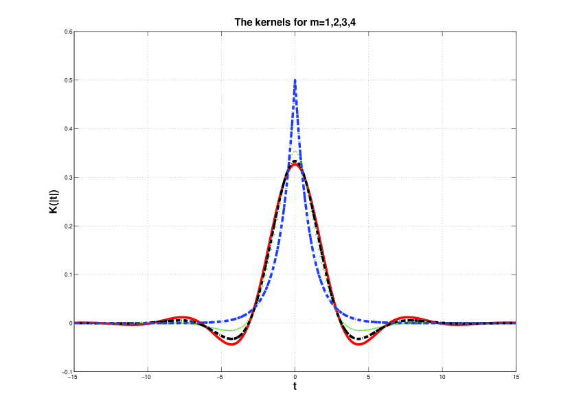
Figure 1: The equivalent kernels for $m=1,2,3,4$: (i) $m=1$: the dashed line; (ii) $m=2$: the dotted line; (iii) $m=3$: the dashdot line; (iv) $m=4$: the solid line.

Example 3.1.

As an illustration, the closed-form expressions of the first four equivalent kernels are given below and their plots are shown in Figure 1, respectively.

$$m=1:\ \ K(t) = \frac{1}{2}e^{-|t|}$$

$$m=2:\ \ K(t) = \frac{1}{2\sqrt{2}}\,e^{-\frac{1}{\sqrt{2}}|t|}\Big{(}\,\cos\frac{|t|}{\sqrt{2}}+\sin\frac{|t|}{\sqrt{2}}\,\Big{)}$$

$$m=3:\ \ K(t) = \frac{1}{6}e^{-|t|}+\,e^{-\frac{1}{2}|t|}\Big{(}\,\frac{1}{6}\cos\frac{\sqrt{3}|t|}{2}+\frac{\sqrt{3}}{6}\sin\frac{\sqrt{3}|t|}{2}\,\Big{)}$$

$$m=4:\ \ K(t) = e^{-0.9239|t|}\Big{(}\,0.2310\cos(0.3827|t|)+0.0957\sin(0.3827|t|)\,\Big{)}$$

$$\,+\,e^{-0.3827|t|}\Big{(}\,0.0957\cos(0.9239|t|)+0.2310\sin(0.9239|t|)\,\Big{)}$$

3.4 Boundary conditions

Recall that the boundary conditions for the ODE (14) are $F^{(i)}(0)=0$, $F^{(i)}(1)=G^{(i)}(1)$, $i=0,\cdots,m-1$. In the following, we consider an even $m$ first. In this case, the homogeneous ODE: $F^{(2m)}+\beta^{2m}F=0$ has the following $2m$ (linearly independent) solutions:

$$e^{-\beta\mu_{k}t}\cos(\beta\omega_{k}t),\ \ \ e^{-\beta\mu_{k}t}\sin(\beta\omega_{k}t),\ \ \ \ e^{-\beta\mu_{k}(1-t)}\cos(\beta\omega_{k}t),\ \ \ e^{-\beta\mu_{k}(1-t)}\sin(\beta\omega_{k}t),$$

where $k=0,\cdots,\frac{m}{2}-1$ and $\mu_{k},\omega_{k}>0$ for the above $k$. The solution to ODE (14) subject to the boundary conditions can be written as

$$F(t)=\underbrace{\int^{1}_{0}L(|t-s|)G(s)ds}_{F_{0}(t)}+J(t),$$ (25)

where

$$J(t)=\sum^{\frac{m}{2}-1}_{k=0}\Big{\{}e^{-\beta\mu_{k}t}\big{[}a_{k}\cos(\beta\omega_{k}t)+b_{k}\sin(\beta\omega_{k}t)\big{]}+e^{-\beta\mu_{k}(1-t)}\big{[}a^{+}_{k}\cos(\beta\omega_{k}t)+b^{+}_{k}\sin(\beta\omega_{k}t)\big{]}\Big{\}},$$ (26)

and the coefficients $a_{k},b_{k},a^{+}_{k},b^{+}_{k}$ are to be determined from the boundary conditions, and the kernel $L$ is given in (15). Define $\displaystyle\|G\|\equiv\sup_{t\in[0,1]}|G(t)|$. Let ${\bf G}=\big{(}\|G\|,G(1),G^{\prime}(1),\cdots,G^{(m-1)}(1)\big{)}$, and

$${\bf a}\,=\,\Big{(}\,a_{0},b_{0},\cdots,a_{\frac{m}{2}-1},b_{\frac{m}{2}-1},a^{+}_{0},b^{+}_{0},\cdots,a^{+}_{\frac{m}{2}-1},b^{+}_{\frac{m}{2}-1}\,\Big{)}^{T}$$ (27)

be the coefficient vector.

By making use of the boundary conditions, we obtain the linear equation $B^{e}{\bf a}=\bf v$, where ${\bf v}^{T}=[{\bf v_{0}},{\bf v_{1}}]$,

$${\bf v_{0}}=\Big{[}\,-F_{0}(0),\,-\frac{F^{\prime}_{0}(0)}{\beta},\,\cdots,\,-\frac{F^{(m-1)}_{0}(0)}{\beta^{m-1}}\,\Big{]},$$

$${\bf v_{1}}=\Big{[}\,-F_{0}(1)+G(1),\,\frac{-F^{\prime}_{0}(1)+G^{\prime}(1)}{\beta},\,\cdots,\,\frac{-F^{(m-1)}_{0}(1)+G^{(m-1)}(1)}{\beta^{m-1}}\,\Big{]},$$

and

$$B^{e}=\begin{bmatrix}B^{e}_{11}&B^{e}_{12}\\ B^{e}_{21}&B^{e}_{22}\end{bmatrix}.$$

Here the matrix blocks $B^{e}_{ij}\in\mathbb{R}^{m\times m}$ are obtained via the similar technique in Section 3.1 as

$$B^{e}_{11}=$$

$${\small\begin{bmatrix}1&0&1&0&\cdots&\cdots&1&0\\ \cos(\eta_{1})&\sin(\eta_{1})&\cos(3\eta_{1})&\sin(3\eta_{1})&\cdots&\cdots&\cos((m-1)\eta_{1})&\sin((m-1)\eta_{1})\\ \vdots&\vdots&\vdots&\vdots&&&\vdots&\vdots\\ \cos(\eta_{m-1})&\sin(\eta_{m-1})&\cos(3\eta_{m-1})&\sin(3\eta_{m-1})&\cdots&\cdots&\cos((m-1)\eta_{m-1})&\sin((m-1)\eta_{m-1})\end{bmatrix},}$$

where $\eta_{k}=k(\pi-\frac{\pi}{2m}),\,k=1,\cdots,m-1$, and

$$B^{e}_{22}\,=\,$$

$${\small\begin{bmatrix}\cos(\psi_{0,0})&\sin(\psi_{0,0})&\cos(\psi_{1,0})&\sin(\psi_{1,0})&\cdots&\cdots&\cos(\psi_{{m\over 2}-1,0})&\sin(\psi_{{m\over 2}-1,0})\\ \cos(\psi_{0,1})&\sin(\psi_{0,1})&\cos(\psi_{1,1})&\sin(\psi_{1,1})&\cdots&\cdots&\cos(\psi_{{m\over 2}-1,1})&\sin(\psi_{{m\over 2}-1,1})\\ \vdots&\vdots&\vdots&\vdots&&&\vdots&\vdots\\ \cos(\psi_{0,m-1})&\sin(\psi_{0,m-1})&\cos(\psi_{1,m-1})&\sin(\psi_{1,m-1})&\cdots&\cdots&\cos(\psi_{{m\over 2}-1,m-1})&\sin(\psi_{{m\over 2}-1,m-1})\end{bmatrix}},$$

where $\eta^{+}_{k}=\frac{k\pi}{2m}$ for $k=0,\cdots,m-1$, and $\psi_{j,\ell}=\beta\,\omega_{j}+(2j+1)\eta^{+}_{\ell}$ for all $j=0,\cdots,\frac{m}{2},\,\ell=0,\cdots,m-1$, and each entry of $B^{e}_{12}$ and $B^{e}_{21}$ is of order $O(e^{-\beta})$.

Lemma 3.2.

Given an even $m$. There exist positive real numbers $\beta_{*}$ and $\varrho$, dependent on $m$ only, such that for all $\beta\geq\beta_{*}$, the coefficient vector $\bf a$ is unique and satisfies $\|\bf a\|\leq\varrho\,\|\bf G\|$.

Proof.

Note that for $\beta$ sufficiently large, each element of $B^{e}_{12}$ and $B^{e}_{21}$ is sufficiently small. Hence it suffices to show that $B^{e}_{11}$ and $B^{e}_{22}$ are invertible. For this end, let $B^{e}_{11}(k)$ denote the $k$th column of $B^{e}_{11}$. Define $C_{11}\equiv\big{[}B^{e}_{11}(2)\ B^{e}_{11}(1)\ B^{e}_{11}(4)\ B^{e}_{11}(3)\ \cdots\ B^{e}_{11}(m)\ B^{e}_{11}(m-1)\big{]}$. Letting $\vartheta=\frac{\pi}{2m}$, it can be verified that

$$B^{e}_{11}+\imath C_{11}\,=\,$$

$${\footnotesize\begin{bmatrix}1&\imath&1&\imath&\cdots&\cdots&1&\imath\\ -e^{-\imath\vartheta}&-\imath e^{\imath\vartheta}&-e^{-\imath 3\vartheta}&-\imath e^{\imath 3\vartheta}&\cdots&\cdots&-e^{-\imath(m-1)\vartheta}&-\imath e^{\imath(m-1)\vartheta}\\ \vdots&\vdots&\vdots&\vdots&&&\vdots&\vdots\\ (-e^{-\imath\vartheta})^{m-1}&\imath(-e^{\imath\vartheta})^{m-1}&(-e^{-\imath 3\vartheta})^{m-1}&\imath(-e^{\imath 3\vartheta})^{m-1}&\cdots&\cdots&(-e^{-\imath(m-1)\vartheta})^{m-1}&\imath(-e^{\imath(m-1)\vartheta})^{m-1}\end{bmatrix}.}$$

Therefore $B^{e}_{11}+\imath C_{11}$ can be written as $\mbox{diag}(1,\imath,1,\imath,\cdots,1,\imath)V$, where $V$ is an invertible Vandermonde matrix. This implies that $B^{e}_{11}+\imath C_{11}$ is invertible. On the other hand, by noting $C_{11}=B^{e}_{11}J$, where $J=\mbox{diag}\underbrace{(J_{*},\cdots,J_{*})}_{\frac{m}{2}-\mbox{copies}}$ with $J_{*}=\begin{bmatrix}0&1\\ 1&0\end{bmatrix}$, $B^{e}_{11}+\imath C_{11}=B^{e}_{11}(I+\imath J)$. It is easily seen that $I+\imath J$ is invertible, so is $B^{e}_{11}$. To show the invertibility of $B^{e}_{22}$, it is noticed that $B^{e}_{22}=\widetilde{B}^{e}_{22}R$, where $\widetilde{B}^{e}_{22}$ is similar to $B^{e}_{11}$ defined in (3.4) with $\eta_{i}$ replaced by $\eta^{+}_{i}$ and $R=\mbox{diag}\big{(}M(\beta\omega_{0}),M(\beta\omega_{1}),\cdots,M(\beta\omega_{\frac{m}{2}})\big{)}$ where $M(\cdot)$ is given in (22). Clearly $R$ is invertible for all $\beta$, and it can be proved in the similar way as for $B^{e}_{11}$ that $\widetilde{B}^{e}_{22}$ is nonsingular. Hence, $B^{e}_{22}$ is invertible for all $\beta$. Consequently $\det(B^{e})=\det(B^{e}_{11})\det(B^{e}_{22})+O(e^{-m\beta})\neq 0$ for all $\beta$ sufficiently large. In addition, since each entry of the adjoint of $B^{e}$ is bounded, we deduce that $(B^{e})^{-1}=\frac{\mbox{adj}(B^{e})}{\det(B^{e})}$ is bounded and the upper bound depends on $m$ only, where $\mbox{adj}(B^{e})$ stands for the adjoint of $B^{e}$. Furthermore, letting $\kappa=\max_{k}(|c_{k}|,|d_{k}|)$, where $c_{k},d_{k}$ are the coefficients in the kernel $L$, and $\varrho=\min\{\mu_{k},\,k=0,\cdots,\frac{m}{2}-1\}$, we have, for $t_{*}=0$ or $1$,

$$\frac{\big{|}F^{(j)}_{0}(t_{*})\big{|}}{\beta^{j}}\,\leq\,2m\kappa\int^{1}_{0}\beta e^{-\beta\varrho\tau}d\tau\,\|G\|\leq 2m\kappa/\varrho\,\|G\|,\ \ \ \ \forall\ j=1,\cdots,m-1.$$

As a result, the equation $B^{e}x=\bf v$ has a unique solution $\bf a$ that satisfies the desired bound. ∎

Consider an odd $m$. The homogeneous ODE: $F^{(2m)}-\beta^{2m}F=0$ has the following $2m$ (linearly independent) solutions:

$$e^{\pm\beta t},\ \ e^{-\beta\mu_{k}t}\cos(\beta\omega_{k}t),\ \ \ e^{-\beta\mu_{k}t}\sin(\beta\omega_{k}t),\ \ \ \ e^{-\beta\mu_{k}(1-t)}\cos(\beta\omega_{k}t),\ \ \ e^{-\beta\mu_{k}(1-t)}\sin(\beta\omega_{k}t),$$

where $k=1,\cdots,\frac{m-1}{2}$ and $\mu_{k},\omega_{k}>0$ for the above $k$. The solution to ODE (14) subject to the boundary conditions can be written as

$$F(t)\,=\,\underbrace{\int^{1}_{0}P(|t-s|)G(s)ds}_{F_{0}(t)}+J(t),$$ (29)

where

$$J(t) = a_{0}e^{-\beta t}+a^{+}_{0}e^{-\beta(1-t)}+\sum^{\frac{m-1}{2}}_{k=1}\Big{\{}e^{-\beta\mu_{k}t}\big{[}a_{k}\cos(\beta\omega_{k}t)+b_{k}\sin(\beta\omega_{k}t)\big{]}$$ (30)

$$~{}~{}~{}~{}~{}~{}~{}~{}~{}~{}~{}~{}~{}~{}~{}+\ e^{-\beta\mu_{k}(1-t)}\big{[}a^{+}_{k}\cos(\beta\omega_{k}t)+b^{+}_{k}\sin(\beta\omega_{k}t)\big{]}\Big{\}},$$

and the coefficients $a_{k},b_{k},a^{+}_{k},b^{+}_{k}$ are to be determined from the boundary conditions, and the kernel $P$ is given in (19). Let

$${\bf b}\,=\,\Big{(}a_{0},a_{1},b_{1},\cdots,a_{\frac{m-1}{2}},b_{\frac{m-1}{2}},a^{+}_{0},a^{+}_{1},b^{+}_{1},\cdots,a^{+}_{\frac{m-1}{2}},b^{+}_{\frac{m-1}{2}}\Big{)}^{T}$$ (31)

be the coefficient vector. Similar to the case where $m$ is even, we obtain the linear equation $B^{o}{\bf b}=\bf v$, where ${\bf v}^{T}=[{\bf v_{0}},{\bf v_{1}}]$ and

$$B^{o}\,=\,\begin{bmatrix}B^{o}_{11}&B^{o}_{12}\\ B^{o}_{21}&B^{o}_{22}\end{bmatrix}.$$

Here the matrix blocks $B^{o}_{ij}\in\mathbb{R}^{m\times m}$ are obtained via the similar technique in Section 3.2 as

$$B^{o}_{11}\,=\,$$

$${\small\begin{bmatrix}1&1&0&\cdots&\cdots&1&0\\ -1&\cos(\gamma_{1})&\sin(\gamma_{1})&\cdots&\cdots&\cos(\gamma_{\frac{m-1}{2}})&\sin(\gamma_{\frac{m-1}{2}})\\ \vdots&\vdots&\vdots&&&\vdots&\vdots\\ (-1)^{m-1}&\cos((m-1)\gamma_{1})&\sin((m-1)\gamma_{1})&\cdots&\cdots&\cos((m-1)\gamma_{\frac{m-1}{2}})&\sin((m-1)\gamma_{\frac{m-1}{2}})\end{bmatrix},}$$

where $\gamma_{k}=(\pi-\frac{k\pi}{m}),k=1,2,\cdots,\frac{m-1}{2}$, and

$$B^{o}_{22}\,=\,\begin{bmatrix}1&\cos(\zeta_{1,0})&\sin(\zeta_{1,0})&\cdots&\cdots&\cos(\zeta_{\frac{m-1}{2},0})&\sin(\zeta_{\frac{m-1}{2},0})\\ 1&\cos(\zeta_{1,1})&\sin(\zeta_{1,1})&\cdots&\cdots&\cos(\zeta_{\frac{m-1}{2},1})&\sin(\zeta_{\frac{m-1}{2},1})\\ \vdots&\vdots&\vdots&&&\vdots&\vdots\\ 1&\cos(\zeta_{1,m-1})&\sin(\zeta_{1,m-1})&\cdots&\cdots&\cos(\zeta_{\frac{m-1}{2},m-1})&\sin(\zeta_{\frac{m-1}{2},m-1})\end{bmatrix},$$

where $\gamma^{+}_{k}=\frac{k\pi}{m},\,\zeta_{k,\ell}=\beta\,\omega_{k}+\ell\gamma^{+}_{k}$ for all $k=1,2,\cdots,\frac{m-1}{2},\,\ell=0,1,\cdots,m-1$, and each entry of $B^{o}_{12}$ and $B^{o}_{21}$ is of order $O(e^{-\beta})$. To show the invertibility of $B^{o}_{11}$, we introduce $E_{11}\equiv\big{[}0\ B^{o}_{11}(3)\ B^{o}_{11}(2)\ B^{o}_{11}(5)\ B^{o}_{11}(4)\ \cdots\ B^{o}_{11}(m)\ B^{e}_{11}(m-1)\big{]}$, where $B^{o}_{11}(k)$ denotes the $k$th column of $B^{o}_{11}$. As before it can be shown that $B^{o}_{11}+\imath E_{11}$ is nonsingular and $B^{o}_{11}+\imath E_{11}=B^{o}_{11}(I+\imath K)$, where $K\equiv\mbox{diag}(0,\underbrace{J_{*},\cdots,J_{*}}_{\frac{m-1}{2}-\mbox{copies}})$ and $J_{*}$ is the $2\times 2$ matrix defined before. Since $I+\imath K$ is nonsingular, so is $B^{o}_{11}$. Furthermore, by applying the similar technique, we can show that $B^{o}_{22}$ is invertible for all $\beta$. This thus implies that for all $\beta$ sufficiently large, $B^{o}$ is invertible and each entry of $(B^{o})^{-1}$ is bounded by a positive number depending on $m$ only. We summarize the above discussions as follows:

Lemma 3.3.

Given an odd $m$. There exist positive real numbers $\beta_{*}$ and $\varrho$, dependent on $m$ only, such that for all $\beta\geq\beta_{*}$, the coefficient vector $\bf b$ is unique and satisfies $\|\bf b\|\leq\varrho\,\|\bf G\|$.

4 Asymptotic properties of $P$-splines

To establish the asymptotic properties of the estimator, we first represent $\hat{F}_{m}$ as the sum of the convolutions of $K(t,s)$ (defined in Section 3) with $G_{m}$ and a remainder term that is of smaller order.

Lemma 4.1.

The $\hat{F}_{m}$ in (13) can be represented as

$$\hat{F}_{m}(t)=\int_{0}^{1}K(s,t)G_{m}(s)ds+\int_{0}^{1}K(s,t)\tilde{R}(s)ds+J(t),$$ (33)

where $J(t)$ is given by (26) and (30) for even $m$ and odd $m$, respectively. The $\|\cdot\|_{\infty}$-norms of both coefficient vectors ${\bf a}$ in (27) and ${\bf b}$ in (31) are stochastically bounded, and $\|\tilde{R}\|=O_{p}\Big{(}\big{(}{\log K_{n}\over nK_{n}}\big{)}^{1/2}\Big{)}$.

Proof.

The representation of $\hat{F}_{m}$ in (33) follows from the discussions in Section 3. The stochastic boundedness of the coefficient vectors is the direct applications of Lemma 3.2 and Lemma 3.3. Let $\bar{y}={K_{n}\over n}X^{T}y$ and $\lambda=\lambda^{*}K_{n}/n$. Claeskens et al. (2009) showed that $\|H^{-1}\|_{\infty}=O(1)$, where $H={K_{n}\over n}X^{T}X+\lambda D^{T}_{m}D_{m}$. Thus, $\hat{b}$ is stochastically bounded, so is $\hat{f}^{[p]}$. Let $\bar{b}$ solve $(X^{T}X+\lambda^{*}D_{m}^{T}D_{m})\bar{b}=X^{T}f$ and denote $\bar{f}(x)=\sum_{k=1}^{K_{n}+p}\bar{b}_{k}B_{k}^{(p)}(x)$. We have

$$\|\hat{f}^{[p]}-\bar{f}\|\,\leq\,\|\hat{b}-\bar{b}\|_{\infty}\,\leq\,\|H^{-1}\|_{\infty}\,\|\ \bar{y}-\mathbb{E}[\bar{y}]\ \|_{\infty}\,=\,O_{p}\Big{(}\sqrt{K_{n}\over n}\sqrt{2\log K_{n}}~{}\Big{)}.$$ (34)

It is shown that $\|\bar{f}-f\|=O(\alpha)$ if $p=m$. The development of this result is a special case of Theorem 4.1 in Section 4. Thus,

$$|\hat{F}_{1}(x)-G_{1}(x)+G_{1}(\kappa_{k_{x}+p})-\check{F}_{1}(\kappa_{k_{x}+p})|$$

$$\leq |\hat{F}_{1}(x)-\check{F}_{1}(x)|+|(G_{1}(\kappa_{k_{x}+p})-G_{1}(x))-(\Phi_{1}(\kappa_{k_{x}+p})-\Phi_{1}(x))|$$

$$+|(\Phi_{1}(\kappa_{k_{x}+p})-\Phi_{1}(x))-(\bar{F}_{1}(\kappa_{k_{x}+p})-\bar{F}_{1}(x))|+|(\bar{F}_{1}(\kappa_{k_{x}+p})-\bar{F}_{1}(x))-(\check{F}_{1}(\kappa_{k_{x}+p})-\check{F}_{1}(x))|$$

$$\leq {2\over n}\|\hat{f}\|+O_{p}\Big{(}{1\over\sqrt{nK_{n}}}\Big{)}+{pM_{n}\over n}\|\bar{f}-f\|+{pM_{n}\over n}\|\hat{f}-\bar{f}\|$$

$$= O_{p}\Big{(}\,{1\over n}\,\Big{)}+O_{p}\Big{(}\big{(}{\log K_{n}\over nK_{n}}\big{)}^{1/2}\Big{)}+O_{p}\Big{(}{\alpha\over K_{n}}\Big{)}.$$

A similar rate can be obtained for $|R_{y,k_{x}+1}-R_{f,k_{x}+1}|$. Given the admissible ranges of $K_{n}$ and $\alpha$ in next Corollary 4.2, $O_{p}(({\log K_{n}/nK_{n}})^{1/2})$ is the dominating term. Hence, the lemma follows. ∎

Theorem 4.1.

If the true regression function is $2m$th order continuously differentiable with bounded $2m$th derivative, then the $P$-spline estimator $\hat{f}^{[m]}$ can be written as

$$\hat{f}^{[m]}(t) = f(t)+(-1)^{m-1}\alpha f^{(2m)}(t)+o(\alpha)+{1\over n}\sum_{i=1}^{n}K(t,t_{i})\epsilon_{i}$$

$$~{}~{}~{}~{}~{}~{}~{}~{}~{}~{}~{}~{}~{}~{}~{}~{}~{}~{}~{}~{}~{}~{}~{}~{}+O_{p}\Big{(}\sqrt{\log K_{n}\over nK_{n}}~{}\Big{)}\beta^{m}+e^{-\beta t(1-t)}O_{p}(\beta^{m}),$$

uniformly in $\alpha$ and in $t\in(0,1)$.

Proof.

Taking the $m$th derivative of $\int_{0}^{1}K(s,t)G_{m}(s)ds$, we obtain

$$\int_{0}^{1}{\partial^{m}K(t,s)\over\partial t^{m}}G_{m}(s)ds = \int_{0}^{1}{\partial^{m}K(t,s)\over\partial t^{m}}\Phi_{m}(s)ds+\int_{0}^{1}{\partial^{m}K(t,s)\over\partial t^{m}}\Big{[}G_{m}(s)-\tilde{\Phi}_{m}(s)\Big{]}ds$$

$$+\int_{0}^{1}{\partial^{m}K(t,s)\over\partial t^{m}}\Big{[}\tilde{\Phi}_{m}(s)-\Phi_{m}(s)\Big{]}ds.$$

It is easy to show that

$$\int_{0}^{1}{\partial K(t,s)\over\partial t}\Phi_{m}(s)ds=-\int_{0}^{1}{\partial K(t,s)\over\partial s}\Phi_{m}(s)ds=-\Phi_{m}(1)K(t,1)+\int_{0}^{1}K(t,s)\Phi_{m-1}(s)ds.$$

Therefore,

$$\int_{0}^{1}{\partial^{m}K(t,s)\over\partial t^{m}}\Phi_{m}(s)ds=-\sum_{j=0}^{m-1}\Phi_{m-j}(1){\partial^{m-j}\over\partial t^{(m-j)}}K(t,1)+\int_{0}^{1}K(t,s)f(s)ds.$$

By Equation (6.4) in Theorem 2.2 of Nychka (1995), we have

$$\int_{0}^{1}K(t,s)f(s)ds=f(t)+(-1)^{m-1}\alpha f^{(2m)}(t)+o(\alpha).$$

Similarly,

$$\int_{0}^{1}{\partial^{m}K(t,s)\over\partial t^{m}}\Big{[}G_{m}(s)-\tilde{\Phi}_{m}(s)\Big{]}ds = -\sum_{j=0}^{m-1}\Big{[}G_{m-j}(1)-\tilde{\Phi}_{m-j}(1)\Big{]}{\partial^{m-j}\over\partial t^{(m-j)}}K(t,1)$$

$$+\int_{0}^{1}K(t,s)\Big{[}dG_{1}(s)-d\tilde{\Phi}_{1}(s)\Big{]},$$

$$= O_{p}\Big{(}{\beta^{m}e^{-\beta(1-t)\over\sqrt{n}}}\Big{)}+{1\over n}\sum_{i=1}^{n}K(t,t_{i})\epsilon_{i}.$$

Moreover,

$$\Big{|}\int_{0}^{1}{\partial^{m}K(t,s)\over\partial t^{m}}\Big{[}\tilde{\Phi}_{m}(s)-\Phi_{m}(s)\Big{]}ds\Big{|}\leq\|\tilde{\Phi}_{m}-\Phi_{m}\|~{}~{}\Big{|}\int_{0}^{1}{\partial^{m}K(t,s)\over\partial t^{m}}ds\Big{|},$$

which is of order $O(1/n)\beta^{m}$. Finally, in light of Lemma 4.1, $\|{d^{m}\over dt^{m}}\int_{0}^{1}K(s,t)\tilde{R}(s)ds\|$ is of order $(\log K_{n}/nK_{n})^{1/2}\beta^{m}$. It is easy to verify that the $m$th derivative of $J(t)$ is of order $e^{-\beta t(1-t)}\beta^{m}$. This completes the detail of the representation. ∎

Remark 4.1.

Theorem 4.1 indicates that the $P$-spline estimator is approximately a kernel regression estimator. The equivalent kernel is $K(t,s)$ given in Section 3, and $\alpha$ plays a role similar to the bandwidth $h$. The asymptotic mean has the bias $(-1)^{m-1}\alpha f^{(2m)}(x)$, which can be negligible if $\alpha$ is reasonably small. On the other hand, $\alpha$ can not be arbitrarily small as that will inflate the random component. The admissible range for $\alpha$ given in Corollary 4.1 is a compromise between these two.

Corollary 4.1.

Let $\alpha$ satisfy $\alpha n^{2m/(4m+1)}\rightarrow 0$ and $\alpha^{-(2m-1)/2m}\log K_{n}/K_{n}\rightarrow 0$. Suppose also that the true regression function $f$ is $2m$th order continuously differentiable with bounded $2m$th derivative. Then for $t\in(0,1)$,

$$\sqrt{n\over\beta}~{}[\hat{f}^{[m]}(t)-f(t)]\rightarrow^{d}N\big{(}0,\sigma_{K}^{2}(t)\big{)},$$ (36)

where ${1\over\beta}\int_{0}^{1}K^{2}(t,s)ds\rightarrow\sigma_{K}^{2}(t)$ as $n\rightarrow\infty$. However, if $\alpha=c^{2m}n^{-{2m\over 4m+1}}$ for $c>0$, and let $K_{n}\sim n^{\gamma}$ with $\gamma>(2m-1)/(4m+1)$, then

$$n^{2m/(4m+1)}~{}[\hat{f}^{[m]}(t)-f(t)]\rightarrow^{d}N\Big{(}(-1)^{m-1}c^{2m}f^{(2m)}(t),~{}~{}{\sigma_{K}^{2}(t)\over c}~{}\Big{)}.$$ (37)

Proof.

Let $\Pi(t)={1\over n}\sum_{i=1}^{n}K(t,t_{i})\epsilon_{i}$. For any fixed $t$, the Lindeberg-Levy central limit theorem gives

$$\sqrt{n\over\beta}~{}\Pi(t)\rightarrow N(0,\sigma_{K}^{2}(t))$$

in distribution, where ${1\over\beta}\int_{0}^{1}K^{2}(t,s)ds\rightarrow\sigma_{K}^{2}(t)$ as $n\rightarrow\infty$. If $\alpha$ satisfies $\alpha n^{2m/(4m+1)}\rightarrow 0$ and $\alpha^{-(2m-1)/2m}\log K_{n}/K_{n}\rightarrow 0$, it is easy to see that the remainder terms in (4.1) are $o_{p}(1)$. If $\alpha=c^{2m}n^{-{2m\over 4m+1}}$ for $c>0$, and $K_{n}\sim n^{\gamma}$ with $\gamma>(2m-1)/(4m+1)$, we have $\sqrt{n/\beta}\alpha=c^{2m+1/2}$ and $\sqrt{n/\beta}\sqrt{\log K_{n}\over nK_{n}}\beta^{m}\rightarrow 0$. The theorem follows. ∎

Remark 4.2.

The asymptotic results in Corollary 4.1 provide theoretical justification of the observation that the number of knots is not important, as long as it is above some minimal level (Ruppert, 2002). It is easy to find that the mean squared error of the $P$-spline estimator is of order $n^{-4m/4m+1}$, which achieves the optimal rate of convergence given in Stone (1982).

In the following, we study the asymptotic property of $\hat{f}^{[p]}(t)=\sum_{k=1}^{K_{n}+p}\hat{b}_{k}B_{k}^{[p]}(t)$ when $p\neq m$. We first define a piecewise $m$th degree polynomial $\tilde{f}^{[m]}$, where $\hat{f}^{[p]}$ and $\tilde{f}^{[m]}$ share the same set of spline coefficients. In particular, define $\tilde{f}^{[m]}(t)=\sum_{k=1}^{K_{n}+m}\hat{b}_{k}B^{[m]}_{k}(t)$ if $p>m$, or $\tilde{f}^{[m]}(t)=\sum_{k=1}^{K_{n}+p}\hat{b}_{k}B^{[m]}_{k}(t)$ if $p<m$. Note that, if $p<m$, $\tilde{f}^{[m]}$ is defined on $[0,1-{m-p\over K_{n}}]$. Following the similar discussion as above, we can establish the asymptotic distribution for $\tilde{f}^{[m]}$ as in (36) and (37), respectively, under different admissible ranges of $\alpha$ and $K_{n}$.

Lemma 4.2.

For any $t\in(0,1)$, let $d=\lfloor K_{n}t\rfloor+1$. Let $\hat{\gamma}(t)=\hat{f}^{[p]}(t)-\tilde{f}^{[m]}(t)$. Then, if $p>m$,

$$\hat{\gamma}(t)=\sum_{q=m+1}^{p}\sum_{i=d+1}^{d+q}\Big{(}{K_{n}\over q}(t-\kappa_{i-q})\Big{)}B_{i}^{[q-1]}(t)\sum_{l=1}^{p}a_{i+1-d,l}K_{n}^{-l}{d^{l}\over dt^{l}}\hat{f}^{[p]}(t),$$ (38)

and if $p<m$,

$$\hat{\gamma}(t)=-\sum_{q=p+1}^{m}\sum_{i=d+1}^{d+m}\Big{(}{K_{n}\over q}(t-\kappa_{i-q})\Big{)}B_{i}^{[q-1]}(t)\sum_{l=1}^{m}b_{i+1-d,l}K_{n}^{-l}{d^{l}\over dt^{l}}\tilde{f}^{[m]}(t),$$ (39)

where the coefficients $\{a_{ij}\}$ and $\{b_{ij}\}$ are constants.

Proof.

The B-spline basis functions have the recurrence relationship such that

$$B_{j}^{[p]}(t)={K_{n}\over p}(t-\kappa_{j-p-1})B_{j-1}^{[p-1]}(t)+{K_{n}\over p}(\kappa_{j}-t)B_{j}^{[p-1]}(t).$$

Let $f^{[p-1]}(t)=\sum_{k=1}^{K_{n}+p-1}b_{k}B_{k}^{[p-1]}(t)$ with the same first $(K_{n}+p-1)$ coefficients of $f^{[p]}$. For $x\in(\kappa_{d},\kappa_{d+1})$, the difference between $f^{[p]}(t)$ and $f^{[p-1]}(t)$ is given by

$${f}^{[p]}(t)-{f}^{[p-1]}(t) = \sum_{i=d+1}^{d+p}\Big{[}b_{i+1}{K_{n}\over p}(t-\kappa_{i-p})+b_{i}\big{(}{K_{n}\over p}(\kappa_{i}-t)-1\big{)}\Big{]}B_{i}^{[p-1]}(t)$$ (40)

$$= \sum_{i=d+1}^{d+p}(b_{i+1}-b_{i})\Big{(}{K_{n}\over p}(t-\kappa_{i-p})\Big{)}B_{i}^{[p-1]}(t).$$

From (40), if $p>m$,

$$\hat{f}^{[p]}(t)=\tilde{f}^{[m]}(t)+\sum_{q=m+1}^{p}\sum_{i=d+1}^{d+q}\Delta b_{i+1}\Big{(}{K_{n}\over q}(t-\kappa_{i-q})\Big{)}B_{i}^{[q-1]}(t).$$

From (2), we have $\Delta^{l}b_{k}=c_{l}^{T}(\Delta b_{k-l+1},\Delta b_{k-l+2},\ldots,\Delta b_{k})$, where

$$c_{l}=\Big{[}~{}(-1)^{l-1}{l-1\choose 0},(-1)^{l-2}{l-1\choose 1},\ldots,(-1)^{0}{l-1\choose l-1}~{}\Big{]}^{T}.$$

Combining this with (7), it is easy to show that there exists $C_{d}\in\mathbb{R}^{p\times p}$ such that

$$\Big{[}~{}\Delta b_{d+2},\Delta b_{d+2},\ldots,\Delta b_{d+p+1}~{}\Big{]}^{T}=C_{d}~{}\Big{[}~{}K_{n}^{-1}{d\over dt}f^{[p]}(t),\ldots,K_{n}^{-p}{d^{p}\over dt^{p}}f^{[p]}(t)~{}\Big{]}^{T}.$$

Hence, we can write

$$\Delta b_{d+k}=\sum_{l=1}^{p}a_{kl}K_{n}^{-l}{d^{l}\over dx^{l}}f^{[p]}(t),\ k=2,\ldots,p+1,$$ (41)

which gives (38). (39) can be established similarly. Thus the lemma follows. ∎

Corollary 4.2.

Suppose that $f$ is $2m$th order continuously differentiable with bounded $2m$th derivative on $[0,1]$. Let $\alpha$ satisfy $\alpha n^{2m/(4m+1)}\rightarrow 0$ and $\alpha^{-(2m-1)/2m}\log K_{n}/K_{n}\rightarrow 0$. Then, for $t\in(0,1)$,

$$\sqrt{n\over\beta}~{}[\hat{f}^{[p]}(t)-f(t)-\hat{\gamma}(t)]\rightarrow^{d}N\big{(}0,\sigma_{K}^{2}(t)\big{)},$$ (42)

where $\gamma(t)$ is given by (38) if $p<m$ or (39) if $p>m$. However, if $\alpha=c^{2m}n^{-{2m\over 4m+1}}$ for $c>0$, and let $K_{n}\sim n^{\gamma}$ with $\gamma>(2m-1)/(4m+1)$, then

$$n^{2m/(4m+1)}~{}[\hat{f}^{[p]}(t)-f(t)-\hat{\gamma}(t)]\rightarrow^{d}N\Big{(}(-1)^{m-1}c^{2m}f^{(2m)}(t),~{}~{}{\sigma_{K}^{2}(t)\over c}~{}\Big{)}.$$ (43)

Remark 4.3.

When $p$ is not equal to $m$, the asymptotic bias has an additional term $\hat{\gamma}(t)$, which is of order $O_{p}(1/K_{n})$. When $K_{n}$ grows sufficiently fast with respect to $n$, this term is asymptotically negligible.

5 The equivalent kernels near boundary

The approximation of the equivalent kernel $K(t,s)$ deteriorates when $t$ is near the boundary points of the design set. In this section, we derive an explicit formula for the equivalent kernel when $t$ is close to the boundary. We discuss the case when $t$ is close to $0$ only; the case when $t$ is close to $1$ follows from the similar argument and thus is omitted.

Consider an even $m$ first. It follows from the closed-form expressions (25) and (26) for $\hat{F}_{m}(t)$ that for $t\in[0,1]$ sufficiently small, the $m$-th derivative of $\sum^{\frac{m}{2}-1}_{k=0}e^{-\beta\mu_{k}(1-t)}\big{[}a^{+}_{k}\cos(\beta\omega_{k}t)+b^{+}_{k}\sin(\beta\omega_{k}t)\big{]}$ is of order $O_{p}(\beta^{m}e^{-\beta})$. Hence, we only consider

$$\widetilde{F}(t)\equiv F_{0}(t)+\sum^{\frac{m}{2}-1}_{k=0}e^{-\beta\mu_{k}t}\big{[}a_{k}\cos(\beta\omega_{k}t)+b_{k}\sin(\beta\omega_{k}t)\big{]}.$$ (44)

In the subsequent, we shall express the coefficients $a_{k},b_{k}$ in terms of $F_{0}(0)$ and its derivatives. This will eventually lead to an explicit expression for the kernel.

In view of (15), we have

$$F^{(j)}_{0}(0)=\int^{1}_{0}\frac{\partial L^{(j)}(|s-t|)}{\partial\,t^{j}}\Big{|}_{t=0}G(s)ds=(-1)^{j}\int^{1}_{0}\frac{\partial L^{(j)}(s)}{\partial\,s^{j}}G(s)ds,\ \ \ \forall\ j=1,\cdots,2m-1.$$ (45)

Moreover, it follows from Section 3.1 that $\displaystyle L(s)=\beta\sum^{\frac{m}{2}-1}_{k=0}p_{k}(s)=\beta\sum^{\frac{m}{2}-1}_{k=0}\begin{bmatrix}\,1&0\end{bmatrix}\begin{bmatrix}p_{k}(s)\\ q_{k}(s)\end{bmatrix}$, where

$$\begin{bmatrix}p_{k}(s)\\ q_{k}(s)\end{bmatrix}=e^{-\beta\mu_{k}s}S(\omega_{k}\beta s)\begin{bmatrix}c_{k}\\ d_{k}\end{bmatrix},$$

and $S(\cdot)\in\mbox{SO}(2)$ is given by $S(\cdot)\,=\,\begin{bmatrix}\cos(\cdot)&\sin(\cdot)\\ -\sin(\cdot)&\cos(\cdot)\end{bmatrix}.$ In light of (17), we have

$$\begin{bmatrix}p^{(j)}_{k}(s)\\ q^{(j)}_{k}(s)\end{bmatrix}=(\beta A_{k})^{j}\begin{bmatrix}p_{k}(s)\\ q_{k}(s)\end{bmatrix}=(\beta A_{k})^{j}e^{-\beta\mu_{k}s}S(\omega_{k}\beta s)\begin{bmatrix}c_{k}\\ d_{k}\end{bmatrix}.$$

As a result, we obtain

$$\frac{\partial L^{(j)}(s)}{\partial\,s^{j}}\,=\,\beta\sum^{\frac{m}{2}-1}_{k=0}\begin{bmatrix}\,1&0\end{bmatrix}\begin{bmatrix}p^{(j)}_{k}(s)\\ q^{(j)}_{k}(s)\end{bmatrix}\,=\,\beta^{j+1}\sum^{\frac{m}{2}-1}_{k=0}(A_{k})^{j}_{1\bullet}e^{-\beta\mu_{k}s}S(\omega_{k}\beta s)\begin{bmatrix}c_{k}\\ d_{k}\end{bmatrix},$$

where $(A_{k})^{j}_{1\bullet}$ denotes the first row of the $j$-th power of $A_{k}$ given in (17). This, along with (45), yields

$$\frac{F^{(j)}_{0}(0)}{\beta^{j}} = (-1)^{j}\int^{1}_{0}\Big{(}\sum^{\frac{m}{2}-1}_{k=0}(A_{k})^{j}_{1\bullet}\beta e^{-\beta\mu_{k}s}S(\omega_{k}\beta s)\begin{bmatrix}c_{k}\\ d_{k}\end{bmatrix}\Big{)}G(s)ds$$

$$= \sum^{\frac{m}{2}-1}_{k=0}(-A_{k})^{j}_{1\bullet}\int^{1}_{0}\Big{(}\beta e^{-\beta\mu_{k}s}S(\omega_{k}\beta s)\begin{bmatrix}c_{k}\\ d_{k}\end{bmatrix}\Big{)}G(s)ds.$$

For notational simplicity, let $\widehat{B}^{e}_{11}$ denote the inverse of the matrix $B^{e}_{11}$ defined in (3.4) and let

$${\bf p}_{j}=\sum^{\frac{m}{2}-1}_{k=0}(-A_{k})^{j}_{1\bullet}\int^{1}_{0}\Big{(}\beta e^{-\beta\mu_{k}s}S(\omega_{k}\beta s)\begin{bmatrix}c_{k}\\ d_{k}\end{bmatrix}\Big{)}G(s)ds,~{}~{}j=0,\cdots,m-1,$$

and ${\bf p}=[{\bf p}_{0},{\bf p}_{1},\cdots,{\bf p}_{m-1}]^{T}\in\,\mathbb{R}^{m}$. Therefore, it follows from the development in Section 3.4 that

$$\begin{bmatrix}a_{0}\\ b_{0}\\ \vdots\\ a_{\frac{m}{2}-1}\\ b_{\frac{m}{2}-1}\end{bmatrix}\,=\,-(\widehat{B}^{e}_{11}+O_{p}(e^{-\beta}))\,{\bf p}\,=\,-\widehat{B}^{e}_{11}\,{\bf p}+O_{p}(e^{-\beta}).$$ (46)

Returning to $\widetilde{F}^{(m)}(t)$ and using (46), we have, for $\beta\rightarrow\infty$,

$$\widetilde{F}^{(m)}(t) = F^{(m)}_{0}(t)+\beta^{m}\sum^{\frac{m}{2}-1}_{\ell=0}(A_{\ell})^{m}_{1\bullet}e^{-\beta\mu_{\ell}t}S(\omega_{\ell}\beta\,t)\begin{bmatrix}a_{\ell}\\ b_{\ell}\end{bmatrix}$$ (47)

$$= \int^{1}_{0}\frac{\partial L^{(m)}(|t-s|)}{\partial\,s^{m}}G(s)ds\,+\,\beta^{m}\,{\bf q}^{T}(t)\Big{(}-\widehat{B}^{e}_{11}\Big{)}{\bf p},$$

where ${\bf q}(t)\equiv\big{[}{\bf q}_{0}(t),{\bf q}_{1}(t),\cdots,{\bf q}_{\frac{m}{2}-1}(t)\big{]}^{T}\in\mathbb{R}^{m}$ with ${\bf q}_{\ell}(t)\equiv(A_{\ell})^{m}_{1\bullet}e^{-\beta\mu_{\ell}t}S(\omega_{\ell}\beta t)\in\mathbb{R}^{1\times 2}$ for $\ell=0,1,\cdots,\frac{m}{2}-1$.

To find the kernel in this case, particularly the kernel for the second term, recall

$$\begin{bmatrix}p_{k}(s)\\ q_{k}(s)\end{bmatrix}=e^{-\beta\mu_{k}s}S(\omega_{k}\beta s)\begin{bmatrix}c_{k}\\ d_{k}\end{bmatrix}.$$

Therefore, the second term in (47) becomes

$$\beta^{m}\,{\bf q}^{T}(t)\Big{(}-\widehat{B}^{e}_{11}\Big{)}{\bf p}\,=\,\int_{0}^{1}W(t,s)G(s)ds,$$

where

$$W(t,s)=\beta^{m}{\bf q}^{T}(t)\,\Big{(}-\widehat{B}^{e}_{11}\Big{)}\begin{bmatrix}\nu_{0}(s)\\ \nu_{1}(s)\\ \vdots\\ \nu_{m-1}(s)\end{bmatrix}$$

and $\nu_{j}(s)=\displaystyle\sum^{\frac{m}{2}-1}_{k=0}(-A_{k})^{j}_{1\bullet}\Big{(}\beta\begin{bmatrix}p_{k}(s)\\ q_{k}(s)\end{bmatrix}\Big{)}$, $j=0,\ldots,m-1$.

Denote by $\overline{p}^{(r)}_{k}(s)$ and $\overline{q}^{(r)}_{k}(s)$ the $r$-th order integrals of $p_{k}(s)$ and $q_{k}(s)$ respectively, namely,

$$\overline{p}^{(r)}_{k}(s)\equiv\underbrace{\int\cdots\int}_{r-\mbox{copies}}p_{k}\,d\tau_{1}\cdots d\tau_{r},\ \ \ \ \overline{q}^{(r)}_{k}(s)\equiv\underbrace{\int\cdots\int}_{r-\mbox{copies}}q_{k}\,d\tau_{1}\cdots d\tau_{r}.$$

In light of (17), it is easy to verify that

$$\begin{bmatrix}\overline{p}^{(r)}_{k}(s)\\ \overline{q}^{(r)}_{k}(s)\end{bmatrix}=(\beta A_{k})^{-r}\begin{bmatrix}p_{k}(s)\\ q_{k}(s)\end{bmatrix}=e^{-\beta\mu_{k}s}(\beta A_{k})^{-r}S(\omega_{k}\beta s)\begin{bmatrix}c_{k}\\ d_{k}\end{bmatrix}.$$

Using this and $\displaystyle\frac{\partial^{m}\overline{p}^{(m)}_{k}(s)}{\partial s^{m}}=p_{k}(s),\frac{\partial^{m}\overline{q}^{(m)}_{k}(s)}{\partial s^{m}}=q_{k}(s)$, we have

$$\nu_{j}(s) = \displaystyle\sum^{\frac{m}{2}-1}_{k=0}(-A_{k})^{j}_{1\bullet}\Big{(}\beta\begin{bmatrix}\frac{\partial^{m}\overline{p}^{(m)}_{k}(s)}{\partial s^{m}}\\ \frac{\partial^{m}\overline{q}^{(m)}_{k}(s)}{\partial s^{m}}\end{bmatrix}\Big{)}={\partial^{m}\over\partial s^{m}}\displaystyle\sum^{\frac{m}{2}-1}_{k=0}(-A_{k})^{j}_{1\bullet}\Big{(}\beta\begin{bmatrix}\overline{p}^{(m)}_{k}(s)\\ \overline{q}^{(m)}_{k}(s)\end{bmatrix}\Big{)}$$

$$= {\partial^{m}\over\partial s^{m}}\displaystyle\sum^{\frac{m}{2}-1}_{k=0}(-A_{k})^{j}_{1\bullet}\Big{(}\beta e^{-\beta\mu_{k}s}(\beta A_{k})^{-m}S(\omega_{k}\beta s)\begin{bmatrix}c_{k}\\ d_{k}\end{bmatrix}\Big{)}.$$

Therefore,

$$W(t,s)\,\equiv\,{\partial^{m}\over\partial s^{m}}\Big{(}{\bf q}^{T}(t)\,\big{(}-\widehat{B}^{e}_{11}\big{)}~{}{\bf r}(s)\Big{)},$$ (48)

where ${\bf r}(s)=[{\bf r}_{0}(s),{\bf r}_{1}(s),\ldots,{\bf r}_{m-1}(s)]^{T}\in\mathbb{R}^{m}$, and

$${\bf r}_{j}(s)=\sum^{\frac{m}{2}-1}_{k=0}(-A_{k})^{-(m-j)}_{1\bullet}\beta e^{-\beta\mu_{k}s}S(\omega_{k}\beta s)\begin{bmatrix}c_{k}\\ d_{k}\end{bmatrix},~{}~{}~{}~{}j=0,\ldots,m-1.$$

Here the coefficients $c_{k},d_{k}$ satisfy the linear equation (18). Finally, we obtain the equivalent kernel for $t\geq 0$ sufficiently small (when $\beta\rightarrow\infty$) as

$$K_{b}(t,s)=L(|t-s|)+{\bf q}^{T}(t)\,\big{(}-\widehat{B}^{e}_{11}\big{)}~{}{\bf r}(s).$$ (49)

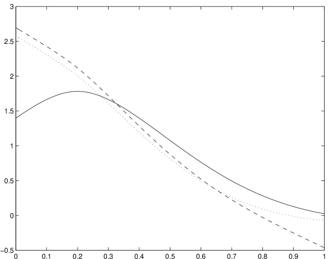
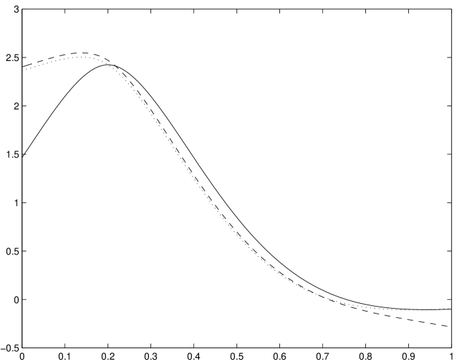
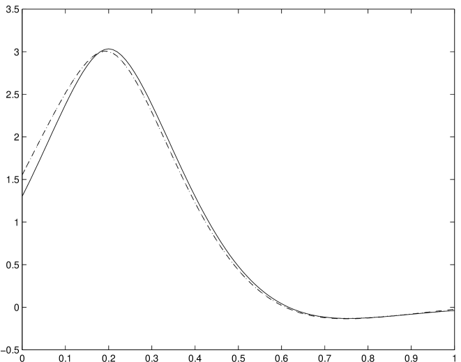
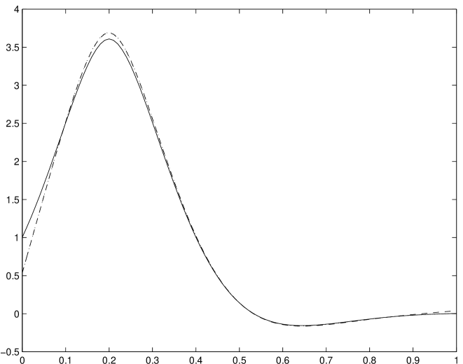
Figure 2: The non-boundary kernel (solid), the finite-sample kernel (dashed) and asymptotic boundary kernel (dotted) for $m=2$ and for (a) $\beta=4$, (b) $\beta=6$, (c) $\beta=8$, (d) $\beta=10$. The kernels are for estimation at $x=0.2$.

Example 5.1.

As an illustration, we derive the closed-form expression of the kernel near the boundary $t=0$ for $m=2$ and compare it with the boundary kernel established by Silverman (1984) for the smoothing splines. Since $c_{0}=d_{0}=\frac{1}{2\sqrt{2}}$,

$$A_{0}\,=\,\begin{bmatrix}\cos(\frac{3\pi}{4})&\sin(\frac{3\pi}{4})\\ -\sin(\frac{3\pi}{4})&\cos(\frac{3\pi}{4})\end{bmatrix},\ \ \ \ S(\omega_{0}\beta t)\,=\,\begin{bmatrix}\cos(\frac{\beta t}{\sqrt{2}})&\sin(\frac{\beta t}{\sqrt{2}})\\ -\sin(\frac{\beta t}{\sqrt{2}})&\cos(\frac{\beta t}{\sqrt{2}})\end{bmatrix},\ \ \ \ \widehat{B}^{e}_{11}=\begin{bmatrix}1&0\\ 1&\sqrt{2}\end{bmatrix},$$

we have

$${\bf q}(t)=e^{-\frac{\beta t}{\sqrt{2}}}\begin{bmatrix}\sin(\frac{\beta t}{\sqrt{2}})\\ -\cos(\frac{\beta t}{\sqrt{2}})\end{bmatrix},~{}~{}~{}~{}~{}{\bf r}(t)=\frac{\beta}{2\sqrt{2}}\,e^{-\frac{\beta s}{\sqrt{2}}}\begin{bmatrix}-\sin(\frac{\beta s}{\sqrt{2}})+\cos(\frac{\beta s}{\sqrt{2}})\\ \sqrt{2}\cos(\frac{\beta s}{\sqrt{2}})\end{bmatrix}.$$

Hence, the equivalent kernel near the boundary $t=0$ is

$$K_{b}(t,s)=L(|t-s|)+{\bf q}^{T}(t)\,\Big{(}-\widehat{B}^{e}_{11}\Big{)}~{}{\bf r}(s)$$

$$= L(|t-s|)\,+\,\frac{\beta}{2\sqrt{2}}\,e^{-\frac{\beta}{\sqrt{2}}(t+s)}\Big{[}\cos\big{(}\frac{\beta}{\sqrt{2}}(t-s)\big{)}+2\cos\big{(}\frac{\beta}{\sqrt{2}}t\big{)}\cos\big{(}\frac{\beta}{\sqrt{2}}s\big{)}-\sin\big{(}\frac{\beta}{\sqrt{2}}(t+s)\big{)}\Big{]}.$$

When $t=0$, since $L(|t-s|)=\frac{\beta}{2\sqrt{2}}\,e^{-\frac{\beta}{\sqrt{2}}s}\big{[}\cos(\frac{\beta}{\sqrt{2}}s)+\sin(\frac{\beta}{\sqrt{2}}s)\big{]}$, the boundary kernel becomes $\sqrt{2}\,e^{-\frac{\beta}{\sqrt{2}}s}\cos(\frac{\beta}{\sqrt{2}}s),\ s\in[0,1]$. It is interesting to notice that the boundary kernel in (5.1) agrees with that obtained by Silverman (1984). Figure 2 displays the non-boundary kernel, boundary kernel, and the finite sample kernel when we estimate $x=0.2$ with different choices of $\beta$, where the finite sample kernel is obtained by incorporating the terms containing $e^{-\beta\mu_{k}(1-t)}$ ignored in (44). Indeed, this kernel is given by

$$L(|t-s|)\,+\,\frac{\beta}{2\sqrt{2}}\,e^{-\frac{\beta}{\sqrt{2}}(t+s)}\Big{[}\cos\big{(}\frac{\beta}{\sqrt{2}}(t-s)\big{)}+2\cos\big{(}\frac{\beta}{\sqrt{2}}t\big{)}\cos\big{(}\frac{\beta}{\sqrt{2}}s\big{)}-\sin\big{(}\frac{\beta}{\sqrt{2}}(t+s)\big{)}\Big{]}$$

$$+\frac{\beta}{2}\,e^{-\frac{\beta}{\sqrt{2}}(2-t-s)}\Big{\{}\cos\big{(}\frac{\beta(1-t)}{\sqrt{2}}+\frac{\pi}{4}\big{)}\Big{[}\cos(\frac{\beta(1-s)}{\sqrt{2}})-\sin(\frac{\beta(1-s)}{\sqrt{2}})\Big{]}+\sqrt{2}\cos(\frac{\beta(1-t)}{\sqrt{2}})\cos(\frac{\beta(1-s)}{\sqrt{2}})\Big{\}}.$$

There are a good agreement between the finite-sample and asymptotic kernels when $\beta=6$ and an excellent agreement when $\beta=10$.

The development of the boundary kernel for an odd $m$ is similar and we omit the details here. For notational simplicity, let $\widehat{B}^{o}_{11}$ denote the inverse of the matrix $B^{o}_{11}$ defined in (3.4). we obtain the equivalent kernel for $t\geq 0$ sufficiently small (when $\beta\rightarrow\infty$) as

$$K_{b}(t,s)=P(|t-s|)+{\bf q}^{T}(t)\Big{(}-\widehat{B}^{o}_{11}\Big{)}{\bf r}(s),$$ (51)

where ${\bf q}(t)=\big{[}(-1)^{m}e^{-\beta t},{\bf q}_{1}(t),\ldots,{\bf q}_{{m-1\over 2}}(t)\big{]}^{T}\in\mathbb{R}^{m}$ and ${\bf r}(s)=[{\bf r}_{0}(s),{\bf r}_{1}(s),\ldots,{\bf r}_{m-1}(s)]^{T}\in\mathbb{R}^{m}$, and

$${\bf q}_{\ell}(t) = (A_{\ell})^{m}_{1\bullet}e^{-\beta\mu_{\ell}t}S(\omega_{\ell}\beta t)\in\mathbb{R}^{1\times 2},~{}~{}~{}~{}\ell=1,\ldots,{m-1\over 2},$$

$${\bf r}_{j}(s) = \displaystyle(-1)^{m}c_{0}\beta e^{-\beta s}+\sum^{\frac{m-1}{2}}_{k=1}(-A_{k})^{-(m-j)}_{1\bullet}\beta e^{-\beta\mu_{k}s}S(\omega_{k}\beta s)\begin{bmatrix}c_{k}\\ d_{k}\end{bmatrix},~{}~{}~{}j=0,\ldots,m-1,$$

where the coefficients $c_{k},d_{k}$ satisfy the linear equation (21).

6 Extensions to unequally spaced data and multivariate smoothing

We have so far focused on the equally spaced design case and equally spaced knots. When the design is not equally spaced, one can use the ideas of Stute (1984) and Li and Ruppert (2008). In specific, assume that $x_{i}$’s are in $(a,b)$. Find a smoothing monotone function $\Upsilon$ such that $\Upsilon(x_{i})=i/n$ from $(a,b)$ to $(0,1)$. We use the $P$-spline smoothing to fit $(i/n,y_{i})$, and thus the regression function is give by $f\circ\Upsilon^{-1}$. We place knots at sample quantiles so that there are equal numbers of data points between consecutive knots.

The univariate $P$-splines can be naturally extended to multivariate $P$-splines (Marx and Eilers, 2005). The asymptotic properties can be studied along the same line. Consider the problem of estimating the $\nu$ dimensional function $f(t_{1},\ldots,t_{\nu})$ from noisy observations $y_{i}=f(t_{1i},\ldots,t_{\nu i})+\epsilon_{i}$, $i=1,\ldots,n$. The $P$-spline model approximates $f$ by

$$f(t_{1},\ldots,t_{\nu})=\sum_{k_{1}=1}^{K_{1n}+p_{1}}\cdots\sum_{k_{\nu}=1}^{K_{\nu n}+p_{\nu}}b_{k_{1},\ldots,k_{\nu}}B_{k_{1}}^{[p_{1}]}(t_{1})\cdots B_{k_{\nu}}^{[p_{\nu}]}(t_{\nu}).$$

The spline coefficient $\hat{b}$ subject to the difference penalty are chosen to minimize

$$\sum_{i=1}^{n}\big{[}y_{i}-\sum_{k_{1}=1}^{K_{1n}+p_{1}}\cdots\sum_{k_{d}=1}^{K_{dn}+p_{d}}b_{k_{1},\ldots,k_{d}}B_{k_{1}}^{[p_{1}]}(t_{1i})\cdots B_{k_{d}}^{[p_{d}]}(t_{di})\big{]}^{2}$$

$$~{}~{}~{}~{}~{}~{}~{}~{}~{}~{}~{}~{}~{}~{}~{}~{}~{}~{}~{}~{}~{}~{}~{}~{}~{}~{}~{}~{}~{}~{}~{}~{}~{}~{}+\lambda^{*}\sum_{k_{1}=m_{1}+1}^{K_{1n}+p_{1}}\cdots\sum_{k_{d}=m_{d}+1}^{K_{dn}+p_{d}}\big{[}\Delta^{m_{1},m_{2},\ldots,m_{d}}b_{k_{1},k_{2},\ldots,k_{d}}\big{]}^{2},$$

where the difference operator for $d$ dimensional case is defined as follows:

$$\Delta^{0,\ldots,0}b_{k_{1},\ldots,k_{\nu}} = b_{k_{1},\ldots,k_{\nu}},~{}~{}k_{1}=1,\ldots,K_{1n}+p_{1},\ldots,k_{\nu}=1,\ldots,K_{\nu n}+p_{\nu},$$

$$\Delta^{m_{1},m_{2},\ldots,m_{\nu}}b_{k_{1},k_{2},\ldots,k_{\nu}} = \Delta^{m_{1}-1,m_{2},\ldots,m_{\nu}}b_{k_{1},k_{2},\ldots,k_{\nu}}-\Delta^{m_{1}-1,m_{2},\ldots,m_{\nu}}b_{k_{1}-1,k_{2},\ldots,k_{\nu}}$$

$$= \Delta^{m_{1},m_{2}-1,\ldots,m_{\nu}}b_{k_{1},k_{2},\ldots,k_{\nu}}-\Delta^{m_{1},m_{2}-1,\ldots,m_{\nu}}b_{k_{1},k_{2}-1,\ldots,k_{\nu}}$$

$$= \cdots$$

$$= \Delta^{m_{1},m_{2},\ldots,m_{\nu}-1}b_{k_{1},k_{2},\ldots,k_{\nu}}-\Delta^{m_{1},m_{2},\ldots,m_{\nu}-1}b_{k_{1}-1,k_{2},\ldots,k_{\nu}-1}.$$

For example, consider a two dimensional difference operator when $k_{1}=1$ and $k_{2}=2$:

$$\Delta^{1,2}b_{ks} = \Delta^{0,2}b_{ks}-\Delta^{0,2}b_{k-1,s}$$

$$= [b_{ks}-2b_{k,s-1}+b_{k,s-2}]-[b_{k-1,s}-2b_{k-1,s-1}+b_{k-1,s-2}].$$

Let $X$ be the $n\times\{\Pi_{j=1}^{\nu}(K_{jn}+p_{j})\}$ matrix with $(i,j)$th entry equal to $B_{k_{1}}^{[p_{1}]}(t_{1i})\cdots B_{k_{\nu}}^{[p_{\nu}]}(t_{di})$. Define $D$ as the $\{\Pi_{j=1}^{\nu}(K_{jn}+p_{j}-m_{j})\}\times\{\Pi_{j=1}^{\nu}(K_{jn}+p_{j})\}$ differencing matrix satisfying

$$Db=\left(\begin{array}[]{c}\Delta^{m_{1},\ldots,m_{\nu}}b_{m_{1}+1,\ldots,m_{\nu}+1}\\ \vdots\\ \Delta^{m_{1},\ldots,m_{\nu}}b_{K_{1n}+p_{1},\ldots,K_{\nu n}+p_{\nu}}\\ \end{array}\right).$$

The optimality condition is given by

$$(X^{T}X+\lambda^{*}D^{T}D)\hat{b}=X^{T}y.$$ (52)

Note that $D=D_{m_{1}}\otimes D_{m_{2}}\otimes\cdots\otimes D_{m_{\nu}}$ and $D^{T}D=D_{m_{1}}^{T}D_{m_{1}}\otimes D_{m_{2}}^{T}D_{m_{2}}\otimes\cdots\otimes D_{m_{d}}^{T}D_{m_{d}}$, where “$\otimes$” represents the Kronecker product. We may go though the same procedure as described in this paper. The multivariate $P$-spline smoothing is asymptotically equivalent to kernel smoothing and the equivalent kernel is the Green’s function corresponding to the partial differential equation (PDE):

$$(-1)^{m_{1}+\cdots+m_{d}}\alpha{\partial^{2m_{1}+\cdots+2m_{d}}\over\partial t_{1}^{2m_{1}}\cdots\partial t_{d}^{2m_{d}}}F(t_{1},\ldots,t_{d})+F(t_{1},\ldots,t_{d})=G(t_{1},\ldots,t_{d}),$$ (53)

subject to the boundary conditions:

$${\partial^{k_{1}+\cdots+k_{d}}\over\partial t_{1}^{k_{1}}\cdots\partial t_{d}^{k_{d}}}F(t_{1},\ldots,t_{d})=0,\mbox{~{}if any }t_{i}=0,~{}~{}k_{i}=0,\ldots,m_{i}-1,$$

$${\partial^{k_{1}+\cdots+k_{d}}\over\partial t_{1}^{k_{1}}\cdots\partial t_{d}^{k_{d}}}F(t_{1},\ldots,t_{d})={\partial^{k_{1}+\cdots+k_{d}}\over\partial t_{1}^{k_{1}}\cdots\partial t_{d}^{k_{d}}}G(t_{1},\ldots,t_{d}),\mbox{~{}if any }t_{i}=1,~{}~{}k_{i}=0,\ldots,m_{i}-1.$$

Further study of this issue is beyond the scope of this paper and shall be reported in a future publication.

References

- [1] Claeskens, G., Krivobokova, T. and Opsomer, J. (2009). Asymptotic properties of penalized spline estimators. Biometrika, in print.
- [2] De Boor, C. (2001) A Pratical Guide to Splines. Springer.
- [3] Hall, P. and Opsomer, J.D. (2005). Theory for penalised spline regression. Biometrika, 92, 105-118.
- [4] Li, Y. and Ruppert, D. (2008). On the asymptotics of penalized splines. Biometrika, 95, 415-436.
- [5] Mammen, E. (1991). Estimating a smoothing regression function. Annals of Statistics, 19, 724-740.
- [6] Marx, B. and Eilers, P. (1996). Flexible smoothing with B-splines and penalties (with comments and rejoinder). Statistical Science, 11, 89-121.
- [7] Marx, B. and Eilers, P. (2005). Multidimensional penalized signal regression. Technometrics, 47 13-22.
- [8] Messer, K. (1991). A comparison of a spline estimate to its equivelent kernel estimate. Annals of Statistics, 19, 817-829.
- [9] Nychka, D. (1995). Splines as local smoothers. Annals of Statistics, 23, 1175-1197.
- [10] O’Sullivan, F. (1986). A statistical perspective on ill-posed inverse problems (with Discussion), Statistical Science, 1, 505-527.
- [11] Pal, J. and Woodroofe, M. (2007). Large sample properties of shape restricted regression estimators with smoothness adjuctments. Statistica Sinica, 17, 1601-1616.
- [12] Rice, J. and Rosenblatt, M. (1983). Smoothing splines: regression, derivatives and deconvolution. Annals of Statistics, 11, 141-156.
- [13] Ruppert, D. (2002). Selecting the number of knots for penalized splines. Journal of Computational and Graphical Statisitcs, 11, 735-757.
- [14] Ruppert, D. and Carroll, R. (2000). Spatially-adaptive penalities for spline fitting. Australian & New Zealand Journal of Statistics, 42, 205-224.
- [15] Ruppert, D., Wand, M.P., and Carroll, R.J. (2003). Semiparametric Regression. Cambridge: Cambridge University Press.
- [16] Silverman, B.W. (1984). Spline smoothing: the equivalent variable kernel method. Annals of Statistics, 12, 898-916.
- [17] Shen, J. and Wang, X. (2009). Estimation of shape constrained functions in dynamical systems and its application to genetic networks. Submitted to 2010 American Control Conference.
- [18] Stone, C.J. (1982). Optimal rate of convergence for nonparametric regression. Annals of Statistics, 10, 1040-1053.
- [19] Stute, W. (1984). Asymptotic normality of nearest neighbor regression function estimates. Annals of Statistics, 12, 917-926.
- [20] Wang, X. and Shen, J. (2009). On the asymptotics of monotone -splines. Manuscript.