Magnetic Branes in Brans-Dicke-Maxwell Theory

Abstract

Abstract

We present a new class of magnetic brane solutions in $(n+1)$-dimensional Brans-Dicke-Maxwell theory in the presence of a quadratic potential for the scalar field. These solutions are neither asymptotically flat nor (anti)-de Sitter. Our strategy for constructing these solutions is applying a conformal transformation to the corresponding solutions in dilaton gravity. This class of solutions represents a spacetime with a longitudinal magnetic field generated by a static brane. They have no curvature singularity and no horizons but have a conic geometry with a deficit angle $\delta$. We generalize this class of solutions to the case of spinning magnetic brane with all rotation parameters. We also use the counterterm method and calculate the conserved quantities of the solutions.

I Introduction

It seems likely that the standard model of cosmology, based on Einstein gravity, could not describe the acceleration of the universe expansion correctly Rie . Thus, cosmologists have attended to alternative theories of gravity to explain the accelerated expansion. One of the alternative theories of general relativity, that arose a lot of enthusiasm recently, is the scalar-tensor theory. Scalar-tensor theories are not new and have a long history. The pioneering study on scalar-tensor theories was done by Brans and Dicke several decades ago who sought to incorporate Mach’s principle into gravity BD . According to Brans-Dicke (BD) theory the phenomenon of inertia arises from acceleration with respect to the general mass distribution of the universe. This theory can be regarded as an economic modification of general relativity which accomodates both Mach’s principle and Dirac’s large number hypothesis as new ingredients. This theory is self-consistent, complete and for $\omega>10^{4}$ is consistent with solar system observations, where $\omega$ is a coupling parameter Will ; Bert ; Aca . In recent years this theory got a new impetus as it arises naturally as the low energy limit of many theories of quantum gravity such as superstring theory or Kaluza-Klein theory. In string theory, gravity becomes scalar-tensor in nature. The low-energy effective action of the superstring theory leads to the Einstein gravity, coupled non-minimally to a scalar field. Due to highly nonlinear character of BD theory, a desirable pre-requisite for studying strong field situation is to have knowledge of exact explicit solutions of the field equations. And as black holes are very important both in classical and quantum gravity, many authors have investigated various aspects of them in BD theory Sen . It turned out that the dynamic scalar field in the BD theory plays an important role in the process of collapse and critical phenomenon. The study on the black hole solutions in BD theory have been carried out extensively in the literature Brans ; Hawking ; Cai1 ; Cai2 ; Kim ; Deh1 ; Gao ; SheyAla .

Besides investigating various aspects of black hole solutions in BD theory, there has been a lot of interest in recent years, in studying the horizonless solutions in various gravity theories. Strong motivation for studying such kinds of solutions comes from the fact that they may be interpreted as cosmic strings. Cosmic strings are topological defects which are inevitably formed during phase transitions in the early universe, and their subsequent evolution and observational signatures must therefore be understood. The string model of structure formation may help to resolve one of cosmological mystery, the origin of cosmic magnetic fields TV . There is strong evidence from all numerical simulations for the scaling behavior of the long string network during the radiation-dominated era. Apart from their possible astrophysical roles, topological defects are fascinating objects in their own right. Their properties, which are very different from those of more familiar system, can give rise to a rich variety of unusual mathematical and physical phenomena AV . A short review of papers treating this subject follows. The four-dimensional horizonless solutions of Einstein gravity have been explored in Vil ; Ban . These horizonless solutions Vil ; Ban have a conical geometry; they are everywhere flat except at the location of the line source. The spacetime can be obtained from the flat spacetime by cutting out a wedge and identifying its edges. The wedge has an opening angle which turns to be proportional to the source mass. The extension to include the Maxwell field Bon and the cosmological constant Lem1 ; Lem2 have also been done. The generalization of these asymptotically AdS magnetic rotating solutions of the Einstein-Maxwell equation to higher dimensions Deh2 and higher derivative gravity Deh3 have been also done. In the context of electromagnetic cosmic string, it has been shown that there are cosmic strings, known as superconducting cosmic strings, that behave as superconductors and have interesting interactions with astrophysical magnetic fields Wit2 . The properties of these superconducting cosmic strings have been investigated in Moss . It is also of great interest to generalize the study to the scalar-tensor theory. Attempts to explore the physical properties of the horizonless solutions in dilaton gravity Fer ; Deh4 ; SDR ; DSH ; Sheykhi and three Dia and four Sen1 dimensional BD theory have also been done. Our aim in this paper is to construct $(n+1)$-dimensional horizonless solutions of Brans-Dicke-Maxwell (BDM) theory for an arbitrary value of coupling constant and investigate the effects of the scalar field on the properties of the spacetime such as the deficit angle of the spacetime.

The structure of our paper is as follows. In section II, we present the basic equations and the conformal transformation between the action of the dilaton gravity theory and the BD theory. In section III, we present the metric for the $(n+1)$-dimensional magnetic solutions in BDM theory with longitudinal magnetic field generated by a static source. In section IV, we generalize these solutions to the case of spining branes. In section V, we obtain the conserved quantities of the spacetimes through the use of the counterterm method. The last section is devoted to conclusion.

II Field equations and Conformal Transformations

The action of the $(n+1)$-dimensional BDM theory with one scalar field $\Phi$ and a self-interacting potential $V(\Phi)$ can be written as

$$I_{G}=-\frac{1}{16\pi}\int_{\mathcal{M}}d^{n+1}x\sqrt{-g}\left(\Phi{R}-\frac{\omega}{\Phi}(\nabla\Phi)^{2}-V(\Phi)-F_{\mu\nu}F^{\mu\nu}\right),$$ (1)

where ${R}$ is the scalar curvature, $V(\Phi)$ is a potential for the scalar field $\Phi$, $F_{\mu\nu}=\partial_{\mu}A_{\nu}-\partial_{\nu}A_{\mu}$ is the electromagnetic field tensor, and $A_{\mu}$ is the electromagnetic potential. The factor $\omega$ is the coupling constant. We obtain the equations of motion by varying the action (1) with respect to the gravitational field $g_{\mu\nu}$, the scalar field $\Phi$ and the gauge field $A_{\mu}$. The result is

$$G_{\mu\nu}=\frac{\omega}{\Phi^{2}}\left(\nabla_{\mu}\Phi\nabla_{\nu}\Phi-\frac{1}{2}g_{\mu\nu}(\nabla\Phi)^{2}\right)-\frac{V(\Phi)}{2\Phi}g_{\mu\nu}+\frac{1}{\Phi}\left(\nabla_{\mu}\nabla_{\nu}\Phi-g_{\mu\nu}\nabla^{2}\Phi\right)$$

$$+\frac{2}{\Phi}\left(F_{\mu\lambda}F_{\nu}^{\ \lambda}-\frac{1}{4}F_{\rho\sigma}F^{\rho\sigma}g_{\mu\nu}\right),$$ (2)

$$\nabla^{2}\Phi=-\frac{n-3}{2(n-1)\omega+2n}F^{2}+\frac{1}{2(n-1)\omega+2n}\left((n-1)\Phi\frac{dV(\Phi)}{d\Phi}-(n+1)V(\Phi)\right),$$ (3)

$$\nabla_{\mu}F^{\mu\nu}=0,$$ (4)

where $G_{\mu\nu}$ and $\nabla$ are, respectively, the Einstein tensor and covariant differentiation in the spacetime metric $g_{\mu\nu}$. It is clear that the right hand side of Eq. (2) includes the second derivatives of the scalar field, so it is hard to solve the field equations (2)-(4) directly. Fortunately, we can remove this difficulty by a conformal transformation. Indeed, the BDM theory (1) can be transformed into the Einstein-Maxwell-dilaton theory via the conformal transformation

$$\bar{g}_{\mu\nu}=\Omega^{-2}g_{\mu\nu},$$ (5)

with

$$\Omega^{-2}=\Phi^{\frac{2}{n-1}},$$ (6)

and

$$\alpha=\frac{n-3}{\sqrt{4(n-1)\omega+4n}},\ \ \ \bar{\Phi}=\frac{n-3}{4\alpha}\ln\Phi.$$ (7)

Using this conformal transformation, the action (1) transforms to

$$\bar{I}_{G}=-\frac{1}{16\pi}\int_{\mathcal{M}}d^{n+1}x\sqrt{-\bar{g}}\left({\bar{R}}-\frac{4}{n-1}(\bar{\nabla}\ \bar{\Phi})^{2}-\bar{V}(\bar{\Phi})-e^{-\frac{4\alpha\bar{\Phi}}{n-1}}\bar{F}_{\mu\nu}\bar{F}^{\mu\nu}\right),$$ (8)

where ${\bar{R}}$ and $\bar{\nabla}$ are, respectively, the Ricci scalar and covariant differentiation in the spacetime metric $\bar{g}_{\mu\nu}$, and $\bar{V}(\bar{\Phi})$ is

$$\bar{V}(\bar{\Phi})=\Phi^{-\frac{n+1}{n-1}}V(\Phi).$$ (9)

This action is just the action of the $(n+1)$-dimensional Einstein-Maxwell-dilaton gravity, where $\bar{\Phi}$ is the dilaton field and $\bar{V}(\bar{\Phi})$ is a potential for $\bar{\Phi}$. $\alpha$ is an arbitrary constant governing the strength of the coupling between the dilaton and the Maxwell field. Varying the action (8), we can obtain equations of motion

$$\bar{{R}}_{\mu\nu}=\frac{4}{n-1}\left(\bar{\nabla}_{\mu}\bar{\Phi}\bar{\nabla}_{\nu}\bar{\Phi}+\frac{1}{4}\bar{V}(\bar{\Phi})\bar{g}_{\mu\nu}\right)+2e^{\frac{-4\alpha\bar{\Phi}}{n-1}}\left(\bar{F}_{\mu\lambda}\bar{F}_{\nu}^{\ \lambda}-\frac{1}{2(n-1)}\bar{F}_{\rho\sigma}\bar{F}^{\rho\sigma}\bar{g}_{\mu\nu}\right),$$ (10)

$$\bar{\nabla}^{2}\bar{\Phi}=\frac{n-1}{8}\frac{\partial\bar{V}}{\partial\bar{\Phi}}-\frac{\alpha}{2}e^{\frac{-4\alpha\bar{\Phi}}{n-1}}\bar{F}_{\rho\sigma}\bar{F}^{\rho\sigma},$$ (11)

$$\bar{\nabla}_{\mu}\left(e^{\frac{-4\alpha\bar{\Phi}}{n-1}}\bar{F}^{\mu\nu}\right)=0.$$ (12)

Comparing Eqs. (2)-(4) with Eqs. (10)-(12), we find that if $\left(\bar{g}_{\mu\nu},\bar{F}_{\mu\nu},\bar{\Phi}\right)$ is the solution of Eqs. (10)-(12) with potential $\bar{V}(\bar{\Phi})$, then

$$\left[{g}_{\mu\nu},{F}_{\mu\nu},{\Phi}\right]=\left[\exp\left({\frac{-8\alpha\bar{\Phi}}{(n-1)(n-3)}}\right)\bar{g}_{\mu\nu},\bar{F}_{\mu\nu},\exp\left({\frac{4\alpha\bar{\Phi}}{n-3}}\right)\right],$$ (13)

is the solution of Eqs. (2)-(4) with potential $V(\Phi)$. In this paper we consider the action (1) with a quadratic potential

$$V(\Phi)=2\Lambda\Phi^{2}.$$

Applying the conformal transformation (13), we obtain the potential $\bar{V}(\bar{\Phi})$ in the dilaton gravity theory

$$\bar{V}(\bar{\Phi})=2\Lambda e^{\frac{4\alpha\bar{\Phi}}{n-1}},$$ (14)

which is a Liouville-type potential. Therefore, instead of solving the complicated Eqs. (2)-(4) of BD theory with quadratic potential, we solve the corresponding Eqs. (10)-(12) of the dilaton gravity theory with a Liouville-type potential. Then, by applying the conformal transformations (13) we obtain magnetic brane solutions in BD theory.

III Static Magnetic Branes in BD theory

Here we want to obtain the $(n+1)$-dimensional solutions of Eqs. (2)-(4) which produce longitudinal magnetic fields in the Euclidean submanifold spans by $x^{i}$ coordinates ($i=1,...,n-2$). We assume the following form for the metric

$$d\bar{s}^{2}=-\frac{\rho^{2}}{l^{2}}R^{2}(\rho)dt^{2}+\frac{d\rho^{2}}{f(\rho)}+l^{2}f(\rho)d\phi^{2}+\frac{\rho^{2}}{l^{2}}R^{2}(\rho)dX^{2}{,}$$ (15)

where $dX^{2}={{\sum_{i=1}^{n-2}}}(dx^{i})^{2}$ is the Euclidean metric on the $(n-2)$-dimensional submanifold. The coordinates $x^{i}$’s have dimension of length and range in $(-\infty,\infty)$, while the angular coordinate $\phi$ is dimensionless as usual and ranges in $[0,2\pi]$. The motivation for this metric gauge $[g_{tt}\varpropto-\rho^{2}$ and $(g_{\rho\rho})^{-1}\varpropto g_{\phi\phi}]$ instead of the usual Schwarzschild gauge $[(g_{\rho\rho})^{-1}\varpropto g_{tt}$ and $g_{\phi\phi}\varpropto\rho^{2}]$ comes from the fact that we are looking for a horizonless solution Lem2 . Inserting metric (15) in the field equations (10)-(12) of the dilaton gravity theory, one can show that these equations have solutions of the form SDR

$$f(\rho)=\frac{2\Lambda(\alpha^{2}+1)^{2}b^{2\gamma}}{(n-1)(\alpha^{2}-n)}\rho^{2(1-\gamma)}+\frac{m}{\rho^{(n-1)(1-\gamma)-1}}-\frac{2q^{2}(\alpha^{2}+1)^{2}b^{-2(n-2)\gamma}}{(n-1)(\alpha^{2}+n-2)\rho^{2(n-2)(1-\gamma)}},$$

$$\bar{\Phi}(\rho)=\frac{(n-1)\alpha}{2(1+\alpha^{2})}\ln(\frac{b}{\rho}),$$

$$R(\rho)=e^{2\alpha\bar{\Phi}/(n-1)},$$

$$\bar{F}_{\phi\rho}=\frac{qle^{4\alpha\bar{\Phi}/(n-1)}}{(\rho R)^{n-1}}.$$ (16)

where $\gamma=\alpha^{2}/(\alpha^{2}+1)$, $q$ is the charge parameter of the brane, and $b$ and $m$ are arbitrary constants. Applying the conformal transformation (13), the $(n+1)$-dimensional magnetic solutions of BD theory can be obtained as

$$ds^{2}=-\frac{\rho^{2}}{l^{2}}H^{2}(\rho)dt^{2}+\frac{d\rho^{2}}{V(\rho)}+l^{2}U(\rho)d\phi^{2}+\frac{\rho^{2}}{l^{2}}H^{2}(\rho)dX^{2}{,}$$ (17)

where $U(\rho)$, $V(\rho)$, $H(\rho)$ and $\Phi(\rho)$ are

$$U(\rho) = \frac{2\Lambda(\alpha^{2}+1)^{2}b^{2\gamma(\frac{n-5}{n-3})}}{(n-1)(\alpha^{2}-n)}\rho^{2(1-\frac{\gamma(n-5)}{n-3})}+\frac{mb^{(\frac{-4\gamma}{n-3})}}{\rho^{n-2}}\rho^{\gamma\left(n-1+\frac{4}{n-3}\right)}$$ (18)

$$-\frac{2q^{2}(\alpha^{2}+1)^{2}b^{-2\gamma\left(n-2+\frac{2}{n-3}\right)}}{(n-1)\left(\alpha^{2}+n-2\right)\rho^{2[(n-2)(1-\gamma)-\frac{2\gamma}{n-3}]}},$$

$$V(\rho) = \frac{2\Lambda(\alpha^{2}+1)^{2}b^{2\gamma(\frac{n-1}{n-3})}}{(n-1)(\alpha^{2}-n)}\rho^{2(1-\gamma(\frac{n-1}{n-3}))}+\frac{mb^{(\frac{4\gamma}{n-3})}}{\rho^{n-2}}\rho^{\gamma(n-1-\frac{4}{n-3})}$$ (19)

$$-\frac{2q^{2}(\alpha^{2}+1)^{2}b^{-2\gamma\left(n-2-\frac{2}{n-3}\right)}}{(n-1)(\alpha^{2}+n-2)\rho^{2[(n-2)(1-\gamma)+\frac{2\gamma}{n-3}]}},$$

$$H(\rho) = \left(\frac{b}{\rho}\right)^{\frac{(n-5)\gamma}{n-3}},$$ (20)

$$\Phi(\rho) = \left(\frac{b}{\rho}\right)^{\frac{2(n-1)\gamma}{n-3}}.$$ (21)

The electromagnetic field becomes

$$F_{\phi\rho} = \frac{qlb^{(3-n)\gamma}}{\rho^{(n-3)(1-\gamma)+2}}.$$ (22)

It is worthwhile to note that the scalar field $\Phi(\rho)$ and the electromagnetic field $F_{\phi\rho}$ become zero as $\rho\rightarrow\infty$. As one can see from Eqs. (18) and (19), the solutions are ill-defined for $\alpha=\sqrt{n}$ with $\Lambda\neq 0$ (corresponding to $\omega=-3(n+3)/4n$). In the limiting case $\alpha\rightarrow 0$ ($\omega\rightarrow\infty$), our solutions restore those presented in Deh2 for magnetic branes in Einstein-Maxwell theory.

Next, we study the properties of the solutions. First of all, we seek for curvature singularities. One can easily check that the Kretschmann scalar, $R_{\mu\nu\lambda\kappa}R^{\mu\nu\lambda\kappa}$, diverges at $\rho=0$ and therefore one might think that there is a curvature singularity located at $\rho=0$. However, a profound look at the metric reveals that the spacetime will never achieve $\rho=0$. The function $V(\rho)$ is negative for $\rho<r_{+}$ and positive for $\rho>r_{+}$, where $r_{+}$ is the largest root of $V(\rho)=0$. Indeed, $g_{\rho\rho}$ and $g_{\phi\phi}$ are related by $V(\rho)=g_{\rho\rho}^{-1}\propto l^{-2}g_{\phi\phi}$, and therefore when $g_{\rho\rho}$ becomes negative (which occurs for $\rho<r_{+}$) so does $g_{\phi\phi}$. This leads to apparent change of signature of the metric from $(n-1)+$ to $(n-2)+$ as one extends the spacetime to $\rho<r_{+}$. This indicates that we are using an incorrect extension. To get rid of this incorrect extension, we introduce the new radial coordinate $r$ as

$$r^{2}=\rho^{2}-r_{+}^{2}\Rightarrow d\rho^{2}=\frac{r^{2}}{r^{2}+r_{+}^{2}}dr^{2}.$$

With this new coordinate, the metric (17) becomes

$$ds^{2} = -\frac{r^{2}+r_{+}^{2}}{l^{2}}H^{2}(r)dt^{2}+l^{2}U(r)d\phi^{2}$$ (23)

$$+\frac{r^{2}dr^{2}}{(r^{2}+r_{+}^{2})V(r)}+\frac{r^{2}+r_{+}^{2}}{l^{2}}H^{2}(r)dX^{2},$$

where the coordinates $r$ assumes the values $0\leq r<\infty$, and $U(r)$, $V(r)$, $H(r)$ and $\Phi(r)$ are now given as

$$U(r) = \frac{2\Lambda(\alpha^{2}+1)^{2}b^{2\gamma(\frac{n-5}{n-3})}}{(n-1)(\alpha^{2}-n)}(r^{2}+r_{+}^{2})^{(1-\frac{\gamma(n-5)}{n-3})}+\frac{mb^{(\frac{-4\gamma}{n-3})}}{(r^{2}+r_{+}^{2})^{(n-2)/2}}(r^{2}+r_{+}^{2})^{\left[n-1+\frac{4}{n-3}\right]\gamma/2}$$ (24)

$$-\frac{2q^{2}(\alpha^{2}+1)^{2}b^{-2\gamma\left(n-2+\frac{2}{n-3}\right)}}{(n-1)\left(\alpha^{2}+n-2\right)(r^{2}+r_{+}^{2})^{[(n-2)(1-\gamma)-\frac{2\gamma}{n-3}]}},$$

$$V(r) = \frac{2\Lambda(\alpha^{2}+1)^{2}b^{2\gamma(\frac{n-1}{n-3})}}{(n-1)(\alpha^{2}-n)}(r^{2}+r_{+}^{2})^{[1-\gamma(\frac{n-1}{n-3})]}+\frac{mb^{(\frac{4\gamma}{n-3})}}{(r^{2}+r_{+}^{2})^{(n-2)/2}}(r^{2}+r_{+}^{2})^{\left[n-1-\frac{4}{n-3}\right]\gamma/2}$$ (25)

$$-\frac{2q^{2}(\alpha^{2}+1)^{2}b^{-2\gamma\left(n-2-\frac{2}{n-3}\right)}}{(n-1)(\alpha^{2}+n-2)(r^{2}+r_{+}^{2})^{[(n-2)(1-\gamma)+\frac{2\gamma}{n-3}]}},$$

$$H(r) = \left(\frac{b}{\sqrt{r^{2}+r_{+}^{2}}}\right)^{\frac{(n-5)\gamma}{n-3}},$$ (26)

$$\Phi(r) = \left(\frac{b}{\sqrt{r^{2}+r_{+}^{2}}}\right)^{\frac{2(n-1)\gamma}{n-3}}.$$ (27)

The asymptotic behavior of the spacetime (23) is neither flat nor (anti)-de Sitter. It is easy to check that the Kretschmann scalar does not diverge in the range $0\leq r<\infty$. However, the spacetime has a conic geometry and has a conical singularity at $r=0$. Indeed, there is a conical singularity at $r=0$ since:

$$\lim_{r\rightarrow 0}\frac{1}{r}\sqrt{\frac{g_{\phi\phi}}{g_{rr}}}\neq 1.$$ (28)

That is, as the radius $r$ tends to zero, the limit of the ratio “circumference/radius” is not $2\pi$ and therefore the spacetime has a conical singularity at $r=0$. The canonical singularity can be removed if one identifies the coordinate $\phi$ with the period

$$\textrm{Period}_{\phi}=2\pi\left(\lim_{r\rightarrow 0}\frac{1}{r}\sqrt{\frac{g_{\phi\phi}}{g_{rr}}}\right)^{-1}=2\pi(1-4\mu),$$ (29)

where $\mu$ is given by

$$\mu=\frac{1}{4}\left[1-\left(\frac{1}{2}\frac{ml(\alpha^{2}+n-2)}{\alpha^{2}+1}r_{+}^{(n-1)(\gamma-1)}+\frac{2(1+\alpha^{2})}{(\alpha^{2}-n)}\Lambda lb^{2\gamma}r_{+}^{1-2\gamma}\right)^{-1}\right].$$ (30)

By the above analysis, we conclude that near the origin $r=0$, the metric (23) describes a spacetime which has a conical singularity at $r=0$ with a deficit angle $\delta=8\pi\mu$, which is proportional to the brane tension at $r=0$ ranjbar . In order to investigate the effects of the scalar field on the the deficit angle, we plot in Figs. 1 and 2 the deficit angle $\delta$ versus $\alpha$. These figures show that for $\Lambda<0$ the deficit angle $\delta$ of the spacetime increases with increasing $\alpha$ while for $\Lambda>0$ the deficit angle decreases with increasing $\alpha$. Of course, one may ask for the completeness of the spacetime with $r\geq 0$ (or $\rho\geq r_{+}$). It is easy to see that the spacetime described by Eq. (23) is both null and timelike geodesically complete as in the case of four-dimensional solutions Lem2 ; Hor3 . In fact, one can show that every null or timelike geodesic starting from an arbitrary point can either extend to infinite values of the affine parameter along the geodesic or end on a singularity at $r=0$ SDR .

Now we investigate the casual structure of the spacetime. As one can see from Eqs. (24)-(25), there is no solution for $\alpha=\sqrt{n}$ with a quadratic potential for the scalar field ($\Lambda\neq 0$). The cases with $\alpha>\sqrt{n}$ and $\alpha<\sqrt{n}$ should be considered separately. For $\alpha>\sqrt{n}$, as $r$ goes to infinity, the dominant term in Eqs. (24)-(25) is the second term, and therefore the functions $U(r)$ and $V(r)$ are positive in the whole spacetime, despite the sign of the cosmological constant $\Lambda$, and is zero at $r=0$. Thus, the solution given by Eqs. (23)-(25) exhibits a spacetime with conic singularity at $r=0$. For $\alpha<\sqrt{n}$, the dominant term for large values of $r$ is the first term, and therefore the functions $U(r)$ and $V(r)$ are positive in the whole spacetime for $\Lambda<0$. In this case the solution represents a spacetime with conic singularity at $r=0$. The solution is not acceptable for $\alpha<\sqrt{n}$ with $\Lambda>0$, since the functions $U(r)$ and $V(r)$ are negative for large values of $r$.

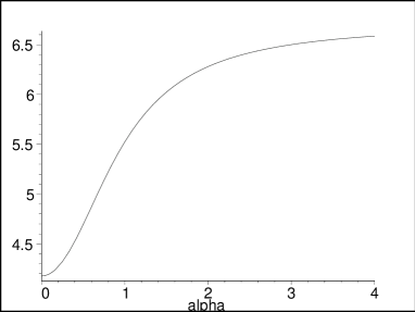
Figure 1: Deficit angle $\delta$ versus $\alpha$ for $n=4$, $b=1$, $l=1$, $\Lambda=-6$, $m=0.3$ and $r_{+}=0.8$.

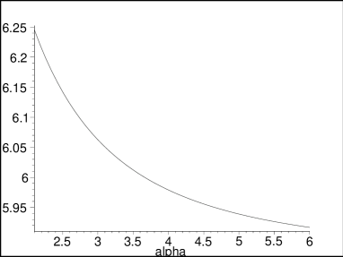
Figure 2: Deficit angle $\delta$ versus $\alpha$ for $n=4$, $b=1$, $l=1$, $\Lambda=+6$, $m=0.3$ and $r_{+}=0.8$.

IV Spinning magnetic Branes in BD theory

In this section, we would like to endow our spacetime metric (17) with a rotation. First, we consider the solutions with one rotation parameter. In order to add an angular momentum to the spacetime, we perform the following rotation boost in the $t-\phi$ plane

$$t\mapsto\Xi t-a\phi,\hskip 14.22636pt\phi\mapsto\Xi\phi-\frac{a}{l^{2}}t,$$ (31)

where $a$ is a rotation parameter and $\Xi=\sqrt{1+a^{2}/l^{2}}$. Substituting Eq. (31) into Eq. (17) we obtain

$$d\bar{s}^{2} = -\frac{r^{2}+r_{+}^{2}}{l^{2}}H^{2}(r)\left(\Xi dt-ad\phi\right)^{2}+\frac{r^{2}dr^{2}}{(r^{2}+r_{+}^{2})V(r)}$$ (32)

$$+l^{2}U(r)\left(\frac{a}{l^{2}}dt-\Xi d\phi\right)^{2}+\frac{r^{2}+r_{+}^{2}}{l^{2}}H^{2}(r)dX^{2}{,}$$

where $U(r)$, $V(r)$ and $H(r)$ are given in Eqs. (24)-(26). The non-vanishing electromagnetic field components become

$$F_{\phi r} = \frac{ql\Xi b^{(3-n)\gamma}}{(r^{2}+r_{+}^{2})^{[(n-3)(1-\gamma)+2]/2}},\hskip 19.91684ptF_{tr}=-\frac{a}{\Xi l^{2}}F_{\phi r}.$$ (33)

The transformation (31) generates a new metric, because it is not a permitted global coordinate transformation. This transformation can be done locally but not globally Sta . Therefore, the metrics (23) and (32) can be locally mapped into each other but not globally, and so they are distinct. Note that this spacetime has no horizon and curvature singularity. However, it has a conical singularity at $r=0$.

Second, we study the rotating solutions with a complete set of rotation parameters. The rotation group in $n+1$ dimensions is $SO(n)$ and therefore the number of independent rotation parameters is $[n/2]$, where $[x]$ is the integer part of $x$. We now generalize the above metric given in Eq. (32) with $k\leq[n/2]$ rotation parameters. This generalized solution can be written as

$$ds^{2} = -\frac{r^{2}+r_{+}^{2}}{l^{2}}H^{2}(r)\left(\Xi dt-{{\sum_{i=1}^{k}}}a_{i}d\phi^{i}\right)^{2}+U(r)\left(\sqrt{\Xi^{2}-1}dt-\frac{\Xi}{\sqrt{\Xi^{2}-1}}{{\sum_{i=1}^{k}}}a_{i}d\phi^{i}\right)^{2}$$ (34)

$$+\frac{r^{2}dr^{2}}{(r^{2}+r_{+}^{2})V(r)}+\frac{r^{2}+r_{+}^{2}}{l^{2}(\Xi^{2}-1)}H^{2}(r){\sum_{i<j}^{k}}(a_{i}d\phi_{j}-a_{j}d\phi_{i})^{2}+\frac{r^{2}+r_{+}^{2}}{l^{2}}H^{2}(r)dX^{2},$$

where $\Xi=\sqrt{1+\sum_{i}^{k}a_{i}^{2}/l^{2}}$, $dX^{2}$ is the Euclidean metric on the $(n-k-1)$-dimensional submanifold with volume $V_{n-k-1}$. The functions $U(r)$, $V(r)$ and $H(r)$ are those presented in Eqs. (24)-(26). The non-vanishing components of electromagnetic field tensor are

$$F_{tr}=-\frac{\Xi^{2}-1}{\Xi a_{i}}F_{\phi^{i}r}=-\frac{q\sqrt{\Xi^{2}-1}b^{(3-n)\gamma}}{(r^{2}+r_{+}^{2})^{[(n-3)(1-\gamma)+2]/2}}.$$ (35)

The corresponding gauge potential of the general solution (34) is given by

$$A_{\mu}=\frac{qb^{(3-n)\gamma}}{\Gamma(r^{2}+r_{+}^{2})^{\Gamma/2}}\left(\sqrt{\Xi^{2}-1}\delta_{\mu}^{t}-\frac{\Xi}{\sqrt{\Xi^{2}-1}}a_{i}\delta_{\mu}^{i}\right)\hskip 14.22636pt{\text{(no sum on }i\text{)}}.$$ (36)

where $\Gamma=(n-3)(1-\gamma)+1$. Again this spacetime has no horizon and curvature singularity. However, it has a conical singularity at $r=0$. One should note that these solutions reduce to those discussed in Deh2 , in the absence of scalar field ($\alpha=\gamma=0$) and those presented in Deh4 for $n=3$.

V Counterterm method and Conserved Quantities

The action (1) does not have a well-defined variational principle, since one encounters a total derivative that produces a surface integral involving the derivative of $\delta g_{\mu\nu}$ normal to the boundary. These normal derivative terms do not vanish by themselves, but are cancelled by the variation of the boundary term

$$I_{b}=-\frac{1}{8\pi}\int_{\partial\mathcal{M}}{d^{n}x\sqrt{h}K\Phi},$$ (37)

where $h$ and $K$ are the determinant of the induced metric and the trace of extrinsic curvature of boundary. In general the action $I_{G}+I_{b}$ , is divergent when evaluated on the solutions. A systematic method of dealing with this divergence for asymptotically AdS solutions of Einstein gravity is through the use of the counterterms method inspired by the anti-de Sitter conformal field theory correspondence (AdS/CFT) Mal . However, in the presence of a non-trivial BD scalar field with potential $V(\Phi)=2\Lambda\Phi^{2}$, the spacetime may not behave as either dS ($\Lambda>0$) or AdS ($\Lambda<0$). In fact, it has been shown that with the exception of a pure cosmological constant potential, where $\alpha=0$, no de Sitter or anti-de Sitter static spherically symmetric solution exist for one Liouville-type dilaton potential PW . But, as in the case of asymptotically AdS spacetimes, according to the domain-wall/QFT (quantum field theory) correspondence Sken , there may be a suitable counterterm for the stress energy tensor which removes the divergences. In this paper, we deal with the spacetimes with zero curvature boundary, and therefore all the counterterm containing the curvature invariants of the boundary are zero. Thus, the suitable counterterm action may be written

$$I_{ct}=-\frac{1}{8\pi}\int_{\partial\mathcal{M}}{d^{n}x\sqrt{h}\frac{(n-1)}{l_{\mathrm{eff}}}},$$ (38)

where $l_{\mathrm{eff}}$ is given by

$$l_{\mathrm{eff}}^{2}=\frac{(n-1)(\alpha^{2}-n)}{2\Lambda\Phi^{3}}.$$ (39)

In the limiting case $\alpha\rightarrow 0$$(\Phi=1)$, the effective $l_{\mathrm{eff}}^{2}$ of Eq. (39) reduces to $l^{2}=-n(n-1)/2\Lambda$ of the AdS spacetimes. Using (37) and (38) the finite stress-energy tensor in $(n+1)$-dimensional BDM theory may be written as

$$T^{ab}=\frac{1}{8\pi}\left[\left(K^{ab}-Kh^{ab}\right)\Phi+\frac{n-1}{l_{\mathrm{eff}}}h^{ab}\right],$$ (40)

The first two terms in Eq. (40) are the variation of the action (37) with respect to $h_{ab}$, and the last term is the counterterm which removes the divergences. Note that the counterterm has the same form as in the case of asymptotically AdS solutions with zero curvature boundary, where $l$ is replaced by $l_{\mathrm{eff}}$. To compute the conserved charges of the spacetime, one should choose a spacelike surface $\mathcal{B}$ in $\partial\mathcal{M}$ with metric $\sigma_{ij}$, and write the boundary metric in ADM (Arnowitt-Deser-Misner) form:

$$\gamma_{ab}dx^{a}dx^{a}=-N^{2}dt^{2}+\sigma_{ij}\left(d\varphi^{i}+V^{i}dt\right)\left(d\varphi^{j}+V^{j}dt\right),$$

where the coordinates $\varphi^{i}$ are the angular variables parameterizing the hypersurface of constant $r$ around the origin, and $N$ and $V^{i}$ are the lapse and shift functions, respectively. When there is a Killing vector field $\mathcal{\xi}$ on the boundary, then the quasilocal conserved quantities associated with the stress tensors of Eq. (40) can be written as

$$Q(\mathcal{\xi)}=\int_{\mathcal{B}}d^{n-1}x\sqrt{\sigma}T_{ab}n^{a}\mathcal{\xi}^{b},$$ (41)

where $\sigma$ is the determinant of the metric $\sigma_{ij}$, $\mathcal{\xi}$ and $n^{a}$ are the Killing vector field and the unit normal vector on the boundary $\mathcal{B}$. For boundaries with timelike ($\xi=\partial/\partial t$) and rotational ($\varsigma_{i}=\partial/\partial\phi^{i}$) Killing vector fields one obtains the quasilocal mass and components of total angular momenta as

$$M = \int_{\mathcal{B}}d^{n-1}x\sqrt{\sigma}T_{ab}n^{a}\xi^{b},$$ (42)

$$J_{i} = \int_{\mathcal{B}}d^{n-1}x\sqrt{\sigma}T_{ab}n^{a}\varsigma_{i}^{b},$$ (43)

provided the surface $\mathcal{B}$ contains the orbits of $\varsigma$. These quantities are, respectively, the conserved mass and angular momenta of the system enclosed by the boundary $\mathcal{B}$. Note that they will both be dependent on the location of the boundary $\mathcal{B}$ in the spacetime, although each is independent of the particular choice of foliation $\mathcal{B}$ within the surface $\partial\mathcal{M}$. Now we are in a position to calculate conserved quantities of the solutions. Denoting the volume of the hypersurface boundary at constant $t$ and $r$ by $V_{n-1}=(2\pi)^{k}\Sigma_{n-k-1}$, the mass and angular momentum per unit volume $V_{n-1}$ of the branes ($\alpha<\sqrt{n}$) can be calculated through the use of Eqs. (42) and (43). We find

$${M} = \frac{b^{(n-1)\gamma}}{16\pi l^{n-2}}\left(\frac{(n-\alpha^{2})\Xi^{2}-(n-1)}{1+\alpha^{2}}\right)m,$$ (44)

$$J_{i} = \frac{b^{(n-1)\gamma}}{16\pi l^{n-2}}\left(\frac{n-\alpha^{2}}{1+\alpha^{2}}\right)\Xi ma_{i}.$$ (45)

For $a_{i}=0$ ($\Xi=1$), the angular momentum per unit volume vanishes, and therefore $a_{i}$’s are the rotational parameters of the spacetime. Comparing the conserved quantities calculated in this section with those obtained in SDR , we find that they are invariant under the conformal transformation (13). In the particular case $n=3$, these conserved quantities reduce to the conserved quantities of the magnetic rotating black string obtained in Ref. Deh4 , and in the absence of dilaton field ($\alpha=0=\gamma$) they reduce to those presented in Ref. Deh2 .

Finally, we calculate the electric charge of the solutions. To determine the electric field we should consider the projections of the electromagnetic field tensor on special hypersurfaces. The normal to such hypersurfaces for the spacetimes with a longitudinal magnetic field is

$$u^{0}=\frac{1}{N},\text{ \ }u^{r}=0,\text{ \ }u^{i}=-\frac{V^{i}}{N},$$

and the electric field is $E^{\mu}=g^{\mu\rho}F_{\rho\nu}u^{\nu}$. Then the electric charge per unit volume $V_{n-1}$ can be found by calculating the flux of the electric field at infinity, yielding

$${Q}=\frac{\sqrt{\Xi^{2}-1}q}{4\pi l^{n-2}}.$$ (46)

It is worth noting that the electric charge of the system per unit volume is proportional to the magnitude of rotation parameters and is zero for the case of a static solution. This result is expected since now, besides the magnetic field along the $\phi^{i}$ coordinates, there is also a radial electric field ($F_{t\rho}\neq 0$). To give a physical interpretation for the appearance of the net electric charge, we first consider the static spacetime. The magnetic field source can be interpreted as composed of equal positive and negative charge densities, where one of the charge density is at rest and the other one is spinning. Clearly, this system produce no electric field since the net electric charge density is zero, and the magnetic field is produced by the rotating electric charge density. Now, we consider the spining solutions. From the point of view of an observer at rest relative to the source ($S$), the two charge densities are equal, while from the point of view of an observe $S^{\prime}$ that follows the intrinsic rotation of the spacetime, the positive and negative charge densities are not equal, and therefore the net electric charge of the spacetime is not zero.

VI Conclusion

To conclude, we found a new class of magnetic solutions in Brans-Dicke-Maxwell theory in the presence of a quadratic potential for the scalar field. These solutions are neither asymptotically flat nor (anti)-de Sitter. This class of solutions represents an $(n+1)$-dimensional spacetime with a longitudinal magnetic field generated by a static magnetic brane. We investigated the properties of these solutions and found that these solutions have no curvature singularity and no horizons, but have conic singularity at $r=0$ with a deficit angle $\delta$. Then, we generalized our solutions to the case of spining magnetic brane with $k\leq[n/2]$ rotation parameters. For the spinning brane, when the rotation parameters are nonzero, the brane has a net electric charge density which is proportional to the magnitude of the rotation parameters given by $\sqrt{\Xi^{2}-1}$. We obtained the the conserved quantities of these spacetimes through the use of counterterm method inspired by (A)dS/CFT correspondence.