Local orientational ordering in fluids of spherical molecules
with dipolar-like anisotropic adhesion.

Abstract

We discuss some interesting physical features stemming from our previous analytical study of a simple model of a fluid with dipolar-like interactions of very short range in addition to the usual isotropic Baxter potential for adhesive spheres. While the isotropic part is found to rule the global structural and thermodynamical equilibrium properties of the fluid, the weaker anisotropic part gives rise to an interesting short-range local ordering of nearly spherical condensation clusters, containing short portions of chains having nose-to-tail parallel alignment which runs antiparallel to adjacent similar chains.

Even simple hard sphere fluids display a non-trivial phase diagram, as a function of the packing fraction, which can be experimentally probed and theoretically interpretedZaccarelli09 . Softening the potential and/or increasing its range, leads to a remarkably richer phase diagram which has attracted considerable attention recently (see e.g. Ref. Zaccarelli08, for a recent review). Yethiraj and van Blaaderen Yethiraj03 have discussed how it is experimentally possible to tune the interactions from hard sphere to soft and dipolar ones. More recently, Lu et al. Lu08 have shown that, contrary to an intuitive expectation, gelation of particles with short-range attractions is intimately connected with its equilibrium phase diagram.

It is widely believed that the addition of a long-range repulsion to a short-range attraction inhibits phase separation, by promoting the formation of an equilibrium gel. The same mechanism can be achieved by reducing the probability of forming a bulk liquid using the concept of limited-valency and/or patchy particles Zaccarelli08 . This idea has been recently explored by a number of authors, who have used the so-called Kern and Frenkel model with circular adhesive patches (of non-vanishing area), or that with short-ranged attractive point-sites on the surface of hard spheres Kern03 ; Fantoni07 ; Liu07 ; Foffi07 ; Bianchi08 ; Gogelein08 ; Tavares09 .

In spite of their usefulness, the above models share a common shortcoming on the discontinuous dependence of the potential on the particle orientations, which makes them very difficult to investigate from a theoretical point of view. This drawback is not present in molecular interactions where this dependence is continuous, as for instance in dipolar interactions Wertheim71 , a case which is particularly interesting for various reasons. First, because of their widespread appearance in colloidal suspensions, such as ferrofluids, which have important practical applications. In addition, recent studies Tlusty00 ; Camp00 ; Ganzenmuller07 have shown the existence of a significant influence, in the equilibrium properties of the fluid, of chain-like aggregation characteristic of the dipolar interaction, which strongly competes with a stable fluid-fluid phase separation.

Motivated by this features, in this paper we then take an extreme alternative of considering a tail with dipolar-like anisotropy combined with a very short-range attraction. The latter is patterned after the well-known Baxter’s sticky hard sphere (SHS) potential, where attraction occurs only at contact Baxter68 . Building upon our previous, almost fully analytical, study on this model within the Percus-Yevick closure with orientational linearization (PY-OL) Gazzillo08 , we discuss here some additional interesting features on the local ordering properties, which were not accounted for in our previous work.

In the same spirit of Baxter’s isotropic counterpart Baxter68 , the model is defined by the following Mayer function Gazzillo08

$$f(1,2)=f_{\mathrm{HS}}(r)+t\ \epsilon(1,2)\ \sigma\delta\left(r-\sigma\right),$$ (1)

where $f_{\mathrm{HS}}(r)=\Theta\left(r-\sigma\right)-1$ is its hard sphere (HS) contribution, $\Theta$ the Heaviside step function ( $\Theta(x<0)=0$, $\Theta(x>0)=1$ ), and the Dirac delta function $\delta\left(r-\sigma\right)$ ensures that the adhesive interaction occurs only at contact ($\sigma$ is the HS diameter). The symbol $i\equiv\left(\mathbf{r}_{i},\Omega_{i}\right)$ (with $i=1,2$) denotes both the position $\mathbf{r}_{i}$ of the molecular center and the orientation $\Omega_{i}$ which combines the usual polar and azimuthal angles $\left(\theta_{i},\varphi_{i}\right)$. Thus we have: $(1,2)=(\mathbf{r}_{12},\Omega_{1},\Omega_{2})=(r,\widehat{\mathbf{r}}_{12},\Omega_{1},\Omega_{2})=(r,\Omega_{r},\Omega_{1},\Omega_{2})$, with $\mathbf{r}_{12}=\mathbf{r}_{2}-\mathbf{r}_{1}$, $r=|\mathbf{r}_{12}|$, and $\Omega_{r}$ being the solid angle associated with $\widehat{\mathbf{r}}_{12}=\mathbf{r}_{12}/r$. Moreover, $t$ is the stickiness parameter, equal to $\left(12\tau\right)^{-1}$ in Baxter’s original notation Baxter68 , which measures the strength of surface adhesion and increases with decreasing temperature.

Finally, the angular dependence of the surface adhesion is expressed through the angular factor

$$\epsilon(1,2)=1+\alpha D(1,2),$$ (2)

including the dipolar function

$$D(1,2)=D(\Omega_{r},\Omega_{1},\Omega_{2})=3(\hat{\mathbf{r}}\cdot\mathbf{u}_{1})(\hat{\mathbf{r}}\cdot\mathbf{u}_{2})-\mathbf{u}_{1}\cdot\mathbf{u}_{2}$$ (3)

Here and in the following, the unit vector $\mathbf{u}_{i\text{ }}$ represents the orientation $\Omega_{i}$ of molecule $i$, while $\hat{\mathbf{r}}$ coincides with $\hat{\mathbf{r}}_{12}=-\hat{\mathbf{r}}_{21}$.

The anisotropic function $\epsilon(1,2)$, which has the same symmetry as the dipolar interaction, modulates the sticky attraction. The requirement $\epsilon(1,2)\geq 0$ along with $-2\leq D(1,2)\leq 2$ enforce the limits $0\leq\alpha\leq\frac{1}{2}$ on the anisotropy degree. This range corresponds to the surface interaction always being attractive. In the isotropic case, one has $\alpha=0$ and $\epsilon(1,2)=1$.

As convolutions of Mayer functions generate correlation functions with a more complex angular dependence Wertheim71 , it is necessary to consider also the angular function

$$\Delta(1,2)=\mathbf{u}_{1}\cdot\mathbf{u}_{2}\text{ },$$ (4)

whose limits of variation are clearly $-1\leq\Delta(1,2)\leq 1$.

We note the difference between the dipolar anisotropic adhesion introduced here and the anisotropy belonging to the class of uniform circular ’sticky patches’ Jackson88 ; Ghonasgi95 ; Sear99 ; Mileva00 ; Kern03 ; Zhang05 ; Fantoni07 . In the latter case, the strength of adhesion is uniform, independent of the contact point inside an attractive patch, whereas in our model the value of  the anisotropic correction $\alpha t\ D(1,2)$ changes with the position of the contact point. Moreover, $D(1,2)$ can assume both positive and negative values, depending on the molecular orientations. Consequently, the strength of adhesion between two particles $1$ and $2$ at contact depends – in a continuous way – on the relative orientation of $\mathbf{u}_{1}$ and $\mathbf{u}_{2}$ as well as on the unit vector $\widehat{\mathbf{r}}_{12}$ of the intermolecular distance. The orientations with $D(1,2)>0$, and thus with $\epsilon(1,2)=1+\alpha\ D(1,2)>1$, correspond to an attraction stronger than the isotropic one (given by $\epsilon(1,2)=1$), whereas the configurations with $D(1,2)<0$, and thus with $\epsilon(1,2)<1$, are characterized by a weaker attraction, which can even reduce to zero (HS limit) in the case of highest anisotropy admissible in the present model, i.e. $\alpha=1/2$.

In particular, we shall focus on a set of parallel and antiparallel configurations with $\Delta(1,2)=\mathbf{u}_{1}\cdot\mathbf{u}_{2}=1$, and $\Delta(1,2)=-1$ respectively. The surface adhesion reaches its maximum value when $\mathbf{u}_{1}=\mathbf{u}_{2}=$ $\widehat{\mathbf{r}}_{12}$, which yields $D(1,2)=2$ and $\epsilon(1,2)=1+2\alpha$ (head-to-tail parallel configuration). On the contrary, the stickiness is minimum, and vanishes for $\alpha=1/2$, when $\mathbf{u}_{1\text{ }}=-$ $\mathbf{u}_{2}=\widehat{\mathbf{r}}_{12}$, which corresponds to $D(1,2)=-2$ and $\epsilon(1,2)=1-2\alpha$ (head-to-head or tail-to-tail antiparallel configurations). The intermediate case of orthogonal configuration ($\mathbf{u}_{2}$ perpendicular to $\mathbf{u}_{1}$) corresponds to $D(1,2)=0,$ which is equivalent to the isotropic SHS interaction.

Introducing the orientational average $\langle\ldots\rangle_{\mathbf{u}}=\left(4\pi\right)^{-1}\int d\mathbf{u}\ldots$ we note the following results

$$\begin{array}[]{c}\left\langle\Delta(1,2)\right\rangle_{\mathbf{u}_{1},\mathbf{u}_{2}}=0\qquad\left\langle D(1,2)\right\rangle_{\mathbf{u}_{1},\mathbf{u}_{2}}=0\\ \\ \left\langle\Delta(1,2)D(1,2)\right\rangle_{\mathbf{u}_{1},\mathbf{u}_{2}}=0\text{ \ \ \ \ and \ \ \ \ \ }\left\langle D^{2}(1,2)\right\rangle_{\mathbf{u}_{1},\mathbf{u}_{2}}=\frac{2}{3}\end{array}$$ (5)

In a previous paper (hereafter referred to as Ref. I) Gazzillo08 , we have analytically solved for this model the Percus-Yevick integral equation with an orientational linearization.

We here recall the main results, referring to Ref. I for details. We start with the molecular Ornstein-Zernike (OZ) integral equation for homogeneous fluids

$$h(1,2)=c(1,2)+\rho\int d\mathbf{r}_{3}\ \left\langle\ c(1,3)\ h(3,2)\ \right\rangle_{\mathbf{u}_{3}}\$$ (6)

where $h(1,2)$ and $c(1,2)$ are the total and direct correlation functions, respectively, and $\rho$ is the number density.

Any angle-dependent correlation function $F(1,2)$ could be expanded in a basis of rotational invariants Gray84 , whose first few terms are

$$F(1,2)=F_{0}(r)+F_{\Delta}(r)\Delta(1,2)+F_{D}(r)D(1,2)+\cdots\text{\ ,}$$ (7)

We stop at the linear terms, assuming Wertheim71 ; Gazzillo08 that the angular basis $\left\{1,\Delta,D\right\}$ is sufficient for our purposes.

The PY-OL closure Gazzillo08 is a combination of the PY closure, i.e. $c^{\mathrm{PY}}=f\left(1+\gamma\right)$, with the linear expansion of $\gamma\equiv h-c$ given by $\gamma^{\mathrm{OL}}(1,2)=\gamma_{0}(r)+\gamma_{\Delta}(r)\Delta(1,2)+\gamma_{D}(r)D(1,2)$, which also neglects the $D\Delta$ and $D^{2\text{ }}$terms stemming from the product $f\gamma$. This leads to

$$c^{\mathrm{PY-OL}}(1,2)=c_{0}(r)+c_{\Delta}(r)\Delta(1,2)+c_{D}(r)D(1,2)$$ (8)

$$\left\{\begin{array}[]{c}c_{0}(r)=f_{\mathrm{HS}}(r)[1+\gamma_{0}(r)]+\Lambda_{0}\ \sigma\delta\left(r-\sigma\right)\\ \\ c_{\Delta}(r)=f_{\mathrm{HS}}(r)\gamma_{\Delta}(r)+\Lambda_{\Delta}\ \sigma\delta\left(r-\sigma\right)\\ \\ c_{D}(r)=f_{\mathrm{HS}}(r)\gamma_{D}(r)+\Lambda_{D}\sigma\delta\left(r-\sigma\right)\end{array}\right.$$ (9)

$$\Lambda_{0}=t\ [1+\gamma_{0}(\sigma)],\text{ \ \ \ \ \ \ }\Lambda_{\Delta}=t\ \gamma_{\Delta}(\sigma),\text{ \ \ \ \ \ \ }\Lambda_{D}=t\ \gamma_{D}(\sigma)+\alpha\Lambda_{0}.$$ (10)

The solution of the OZ equation with the above closure then yields the approximate pair distribution function

$$g^{\mathrm{PY-OL}}(1,2)=1+h^{\mathrm{PY-OL}}(1,2)=g_{0}(r)+h_{\Delta}(r)\Delta(1,2)+h_{D}(r)D(1,2)$$ (11)

$$\left\{\begin{array}[]{c}g_{0}(r)=e_{\mathrm{HS}}(r)[1+\gamma_{0}(r)]+\Lambda_{0}\ \sigma\delta\left(r-\sigma\right)\\ \\ h_{\Delta}(r)=e_{\mathrm{HS}}(r)\gamma_{\Delta}(r)+\Lambda_{\Delta}\ \sigma\delta\left(r-\sigma\right)\\ \\ h_{D}(r)=e_{\mathrm{HS}}(r)\gamma_{D}(r)+\Lambda_{D}\sigma\delta\left(r-\sigma\right)\end{array}\right.$$ (12)

where $g_{0}(r)=1+h_{0}(r)$, and $e_{\mathrm{HS}}(r)=1+f_{\mathrm{HS}}(r)$ is the HS Boltzmann factor.

The first term in Eqs. (9) corresponds to the well known isotropic Baxter’s sticky hard sphere solution Baxter68 and the OZ equation and this closure constitute a self-contained system. The remaining two have a similar form, but they depend in a non-trivial way upon the isotropic term (see Ref. I for details).

It is instructive to consider the behavior of the $g(12)$ assuming that $\widehat{\mathbf{r}}_{12}\cdot\mathbf{u}_{1}=1$. We focus on a generic reference particle 1, with fixed position $\mathbf{r}_{1}$ and orientation $\mathbf{u}_{1}$, and consider a particle 2 located along the straight half-line which originates from $\mathbf{r}_{1}$ and has the same direction as $\mathbf{u}_{1}$ (polar axis). Imagine that 2 has fixed distance $r$ from 1, but can assume all possible orientations $\mathbf{u}_{2}$, which – by axial symmetry – can be described by the single angle $\theta_{12}=\cos^{-1}(\mathbf{u}_{1}\cdot\mathbf{u}_{2})$. Consequently, $g(1,2)$ reduces to: $g(r,\theta_{12})=g_{0}(r)+\left[h_{\Delta}(r)+2h_{D}(r)\right](\mathbf{u}_{1}\cdot\mathbf{u}_{2})$.

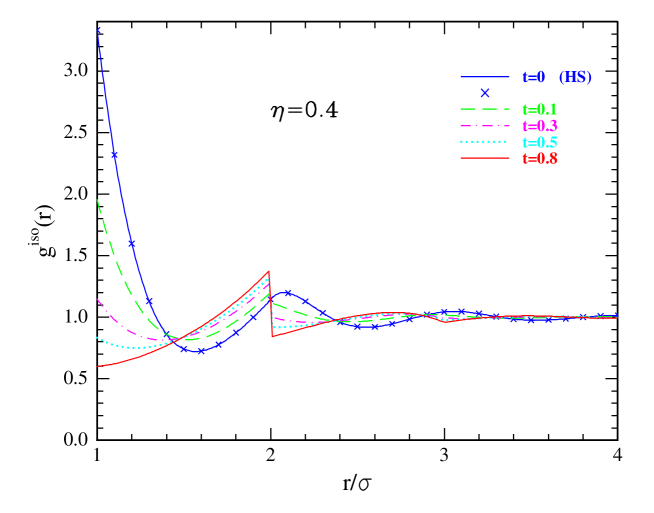
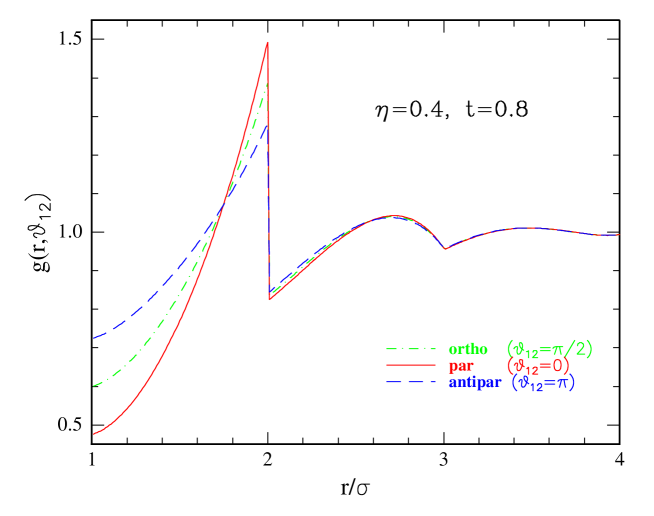
Figure 1: (Color online) (a) Isotropic part of the pair correlation function, $g_{\mathrm{0}}(r)=g^{\mathrm{isoSHS}}(r)$, at $\eta=0.4$, for $t=0,0.1,0.3,0.5,0.8$ corresponding to increasing adhesion strength or decreasing temperature. $t=0$ yields the HS limit. (b) Behavior of $g(r,\theta_{12}),$ when $\alpha=1/2$, at $\eta=0.4$ and $t=0.8,$ for three representative orientations $\theta_{12}=0,\pi/2,\pi$ (parallel, orthogonal and anti-parallel configurations).

Figure 1(a) depicts the behavior of $g_{0}(r)$, which coincides with the reference isotropic part $g^{\mathrm{isoSHS}}(r)$ of the pair correlation function, at $\eta=0.4$.

Here, $t=0$ gives the HS limiting case, $g^{\mathrm{HS}}(r)$, and we consider increasing values of $t$, which correspond to increasing adhesion or decreasing temperature, i.e. $t=0.1,0.3,0.5$ and $0.8$. The last $t$-value yields $\tau=1/(12t)\simeq 0.1$, which lies close to the critical temperature of the isotropic fluid Miller04 .

Two features are noteworthy. First of all, the short-range interactions mainly modify the short-range portions of the pair correlation functions. Very pronounced effects are visible in the range $\sigma<r<2\sigma$, but significant changes are also present all the way out to $r=4\sigma$ and beyond, while the phase of the oscillations is clearly shifted by the addition of the short-range attraction.

A second interesting feature concerns the $t$ dependence of $g_{0}(r)$ in the first shell. As the adhesion strength increases from $t=0$ (HS) to $t=0.8$, the contact value monotonically decreases, whereas a discontinuous peak progressively builds up at $r=(2\sigma)^{-}$. This somewhat counter-intuitive result can be easily understood in terms of the reduction of the pressure exerted on particles 1 and 2 by the surrounding ones in the presence of increasing attraction, thus providing an average larger separation among 1 and 2.

Suppose now that we modulate this attraction with the anisotropic dipolar-like dependence described above. When $\alpha=1/2$ the effect on $g$ is shown in Fig. 1(b) for three representative values of $\theta_{12}$: $\theta_{12}=0$ (parallel orientation), $\theta_{12}=\pi/2$ (orthogonal orientation) and $\theta_{12}=\pi$ (antiparallel orientation). Note that in the orthogonal case the dipolar dependence vanishes and one recovers the isotropic behavior. The main differences occur in the first shell, where the orthogonal curve $\theta_{12}=\pi/2$ is bracketed between the antiparallel ($\theta_{12}=\pi$) and the parallel ($\theta_{12}=0$) results.

Similar qualitative results (with different separations among parallel and antiparallel curves) are found when the angle between $\widehat{\mathbf{r}}_{12}$ and $\mathbf{u}_{1}$ is varied.

From Fig. 1(b) we note that at contact ($r=\sigma^{+}$) the antiparallel configuration is more probable that the nose-to-tail parallel one; conversely, at separations close to $r=2\sigma^{-}$ the parallel alignment is predominant. This can also be confirmed by plotting the projections $h_{\Delta}(r)$ and $h_{D}(r)$ of the molecular correlation function $h^{\mathrm{PY-OL}}(1,2)$ on the angular basis $\Delta(12)$ and $D(12)$ respectively. This is depicted in Fig. 2 where the isotropic corresponding contribution $h_{0}(r)$ is also reported by contrast. One observes a weak negative correlation for both quantities in the region $r\approx\sigma^{+}$ and, conversely, a positive correlation close to $2\sigma^{-}$. A crossing occurs approximately around the same value $r\approx 1.7\sigma$ where the parallel component in Fig. 1(b) overtakes the antiparallel one, as expected.

As we shall see, however, this is a local ordering which does not affect the condensation process.

In order to get more insight into such an orientational ordering, we compute the number of particles with orientation $\mathbf{u}_{2}$ that a generic reference particle 1 with orientation $\mathbf{u}_{1}$ ‘sees’ in an appropriate surrounding volume $V_{AB}$. Assuming $\mathbf{u}_{1}$ as polar axis and taking into account the sphere $S$ with center $\mathbf{u}_{1}$ and radius $R$, $V_{AB}$ is defined as the portion of $S$ corresponding to the solid angle $\Omega_{AB}=\left\{\left(\theta,\varphi\right)\left|\theta_{A}\leq\theta\leq\theta_{B},0\leq\varphi\leq 2\pi\right.\right\}$ (see Fig. 3). Taking for instance $\theta_{A}=0$ and $\theta_{B}=\pi/3$, we can analyze the ‘forward ordering’ as seen by the reference particle, while choice $\theta_{A}=\pi/3$ and $\theta_{B}=\pi/2$ allows to discuss the ‘lateral ordering’.

The number of particles in an infinitesimal spherical cone of height $R=\lambda\sigma$ and infinitesimal solid angle $d\Omega_{r\text{ }}$ in a given direction $\widehat{\mathbf{r}}$ is $d\mathcal{N}\left(\mathbf{u}_{1},\mathbf{u}_{2},\widehat{\mathbf{r}}\right)=d\Omega_{r}\int_{0}^{R}dr\mathbf{\ }r^{2}\ \rho g(1,2),$ where $d\Omega_{r}=d\widehat{\mathbf{r}}$. In a finite solid angle $\Omega_{AB}$

$$\mathcal{N}\left(\mathbf{u}_{1},\mathbf{u}_{2}\right)=\int_{\Omega_{AB}}d\widehat{\mathbf{r}}_{\text{ }}\int_{0}^{R}dr\mathbf{\ }r^{2}\ \rho g(1,2)$$ (13)

Using the first line of equation (5) and equation (11) we see that, within the PY-OL closure, $\left\langle g(12)\right\rangle_{\mathbf{u}_{1},\mathbf{u}_{2}}=g_{0}(r)$, so that the average number is

$$\overline{\mathcal{N}}=\left\langle\mathcal{N}\left(\mathbf{u}_{1},\mathbf{u}_{2}\right)\right\rangle_{\mathbf{u}_{1},\mathbf{u}_{2}}=\rho\ \Omega_{AB}\int_{0}^{R}dr\mathbf{\ }r^{2}\ g_{0}(r)=\rho\ \Omega_{AB}\ \sigma^{3}\ I_{0}$$ (14)

with $\Omega_{AB}=\int_{0}^{2\pi}d\varphi\int_{\theta_{A}}^{\theta_{B}}d\theta\ \sin\theta=2\pi(\cos\theta_{A}-\cos\theta_{B})$ and

$$I_{0}=\left(\lambda^{3}-1\right)/3+\int_{1}^{\lambda}dx\mathbf{\ }x^{2}h_{0\mathrm{,reg}}(x)+\Lambda_{0}$$ (15)

Here we have used the results of Ref. I (see especially Section III D and E), where $h_{0}(r)$ is decomposed into a ‘regular’ term $h_{0\mathrm{,reg}}(r)$ and a ‘singular’ term proportional to the delta function. A similar decomposition is carried out (see again in Ref. I) for the $h_{\Delta}(r)$ and $h_{D}(r)$ parts. Using

$$\left(\Omega_{AB}\right)^{-1}\int_{\Omega_{AB}}d\widehat{\mathbf{r}}\ D(1,2)=\ M_{AB}\left(\mathbf{u}_{1}\cdot\mathbf{u}_{2}\right)$$ (16)

$$M_{AB}=\cos^{2}\theta_{A}+\cos\theta_{A}\cos\theta_{B}+\cos^{2}\theta_{B}-1~{},$$ (17)

we find that the fraction $X$ of particles with orientation $\mathbf{u}_{2}$ in the volume $V_{AB}$ around a reference particle having orientation $\mathbf{u}_{1}$, only depends upon the angle $\theta_{12}=\cos^{-1}(\mathbf{u}_{1}\cdot\mathbf{u}_{2})$ and is given by

$$X(\theta_{12})=\frac{\mathcal{N}\left(\mathbf{u}_{1},\mathbf{u}_{2}\right)}{\overline{\mathcal{N}}}=1+\frac{I_{\Delta}+M_{AB}\ I_{D}}{I_{0}}\ \left(\mathbf{u}_{1}\cdot\mathbf{u}_{2}\right)$$ (18)

$$\begin{array}[]{c}I_{\Delta}=\int_{1}^{\lambda}dx\mathbf{\ }x^{2}h_{\Delta\mathrm{,reg}}(x)+\Lambda_{\Delta}\\ \\ I_{D}=\int_{1}^{\lambda}dx\mathbf{\ }x^{2}h_{D\mathrm{,reg}}(x)+\Lambda_{D}\end{array}$$ (19)

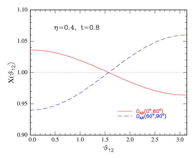
Figure 4: (Color online) (a) Plot of the fraction $X$ of molecules with orientation $\theta_{12}$ contained in the volume $V_{AB\text{ }}$defined by $\sigma\leq r\leq 2\sigma$ and by the solid angle $\Omega_{AB},$ with $\theta_{A}=0,\theta_{B}=\pi/3$ for the forward direction and $\theta_{A}=\pi/3,\theta_{B}=\pi/2$ for the lateral direction. Parameters are: $\alpha=1/2$, $\eta=0.4$ and $t=0.8$ in all cases. (b) Schematic representation of a globular cluster, with internal chain-like orientational ordering.

Fig. 4 (a) depicts $X$ as a function of $\theta_{12}$ in the case $\lambda=2$ (first shell). In the forward region, represented by the solid angle $\Omega_{AB}(0,\pi/3),$ we find $X(0)>X(\pi)$ so there are more particles with parallel orientation, with respect to particle 1. On the contrary, $X(0)<X(\pi)$ in the surrounding lateral region, characterized by $\Omega_{AB}(\pi/3,\pi/2)$, means that here the molecules with antiparallel orientations prevail. Although these effects are rather small, it is reasonable to expect that such differences should grow significantly if the anisotropy parameter $\alpha t$ could become much larger than the strength $t$ of isotropic adhesion. Note that, while $X_{\mathrm{forward}}$ is larger than $X_{\mathrm{lateral}}$ in the interval $0\leq\theta_{12}\leq\pi/2$, an inversion occurs in the region $\pi/2<\theta_{12}\leq\pi$ in agreement with the results of $g(r,\theta_{12})$ reported above (Fig 1 (b)).

The above results are suggestive of the following physical picture. Because of the limits imposed on the anisotropy parameter ($0\leq\alpha\leq 1/2$) by the choice of the potential, the contribution of the dipolar-like interaction is significantly weaker compared to the isotropic part, and does not affect the main condensation process with the formation of globule clusters of nearly isotropic shape. This is in sharp contrast with the purely long-range dipolar models which are mainly characterized by chain-like aggregation Tlusty00 ; Camp00 ; Ganzenmuller07 . However a local ordering occurs within these globular agglomerates of condensation, that are mainly formed by short portions of antiparallel chains running next each other and held together essentially by the isotropic attraction. This is schematically depicted in Fig. 4(b).

We note that only particles belonging to different, antiparallel, chains have direct contact. Consecutive molecules with parallel noise-to-tail orientation – i.e. belonging to the same chain – are not in contact, but lie with average separations slightly smaller than $2\sigma$ as suggested by the behavior of $g$ in Fig.1(b). Thus antiparallel molecules of adjacent chains ’mediate’ an indirect contact between consecutive particles of a given chain.

Once again, we stress that this phenomena should be considered a local fluctuation with very short range (of the order of one shell, as remarked) and does not extend to the entire fluid. This can be readily checked by considering the limit $\lambda\rightarrow\infty$, in which case one finds $I_{D}=0$, so that the dependence from $\mathbf{u}_{1}\cdot\mathbf{u}_{2}=\cos\theta_{12}$ is averaged to zero. As we shall see below, a direct consequence of this is that the coexistence line of the isotropic model is not significantly affected by the anisotropic part, within the PY-OL approximation.

In view of the last remark, one might rightfully wonder whether the anisotropic part plays any role in the thermodynamics of our model. We can convince ourselves that the answer is positive, by considering the exact third virial coefficient as defined by

$$B_{3}=-\frac{1}{3V}\int d\mathbf{r}_{1}~{}d\mathbf{r}_{2}~{}d\mathbf{r}_{3}\ \left\langle f\left(1,2\right)f\left(1,3\right)f\left(2,3\right)\right\rangle_{\mathbf{u}_{1},\mathbf{u}_{2},\mathbf{u}_{3}}$$ (20)

Note that, in view of Eq. (5), the exact second virial coefficient $B_{2}=-\frac{1}{2}\int d\mathbf{r\ }\left\langle f(1,2)\right\rangle_{\mathbf{u}_{1},\mathbf{u}_{2}}$ coincides with its isotropic counterpart. However, this is not the case for $B_{3}$, that can be computed following the method outlined in Ref. Fantoni07, for patchy sticky hard spheres, a close relative to the present model. One finds

$$b_{3}=B_{3}/v_{0}^{2}=10-60t\chi_{1}+144t^{2}\chi_{2}-96t^{3}\chi_{3}~{},$$ (21)

where $v_{0}=\left(\pi/6\right)\sigma^{3}$ and

$$\begin{array}[]{c}\chi_{1}=\langle\epsilon(1,2)\rangle_{\mathbf{u}_{1},\mathbf{u}_{2}}\text{ \ \ \ \ \ \ \ \ \ \ }\chi_{2}=\langle\epsilon(1,2)\epsilon(1,3)\rangle_{\mathbf{u}_{1},\mathbf{u}_{2},\mathbf{u}_{3}}\\ \\ \chi_{3}=\langle\epsilon(1,2)\epsilon(1,3)\epsilon(2,3)\rangle_{\mathbf{u}_{1},\mathbf{u}_{2},\mathbf{u}_{3}}~{}.\end{array}$$ (22)

Again using (5), we find $\chi_{1}=1=\chi_{2}$. The exact value of $\chi_{3}$ turns out to be

$$\chi_{3}=1-\frac{11}{72}\alpha^{3}~{}.$$ (23)

The anisotropic contribution is represented by the term $-(11/72)\alpha^{3}\approx 0.02$, that is very weak with respect to the isotropic one.

Having assessed the limits of the model, we now turn to discuss the limits of the approximation involved in the PY-OL closure. A simple and direct way to quantify its deviation from the exact results is to consider the first order density expansion of the exact direct correlation function $c(1,2)=f(1,2)+c^{(1)}(1,2)\rho+\cdots$. We find

$$c^{(1)}(1,2)=c_{\mathrm{PY-OL}}^{(1)}(1,2)+c_{\mathrm{ex}}^{(1)}(1,2)$$ (24)

with $c_{\mathrm{PY-OL}}^{(1)}(1,2)=c_{0}^{(1)}(r)+c_{\Delta}^{(1)}(r)\ \Delta(1,2)+c_{D}^{(1)}(r)\ D(1,2)$, and

$$c_{\mathrm{ex}}^{(1)}(1,2)=(\alpha t)\ \left[\ \gamma_{\Delta}^{(1)}(\sigma)\ \Delta(1,2)D(1,2)+\gamma_{D}^{(1)}(\sigma)\ D^{2}(1,2)\right]\ \sigma\delta(r-\sigma).$$ (25)

Whereas the PY closure includes both $c_{\mathrm{PY-OL}}^{(1)}(1,2)$ and $c_{\mathrm{ex}}^{(1)}(1,2)$, thus reproducing the exact third virial coefficient through $B_{3}=-\frac{1}{3}\int d\mathbf{r\ }\langle c^{(1)}(1,2)\rangle_{\mathbf{u}_{1},\mathbf{u}_{2}}$, the PY-OL approximation omits the contributions included in $c_{\mathrm{ex}}^{(1)}(1,2)$. Consequently, $b_{3}^{\mathrm{PY-OL}}$ reduces to the purely isotropic contribution: $b_{3}^{\mathrm{iso}}=10-60t+144t^{2}-96t^{3}$. The anisotropic contribution $b_{3}^{\mathrm{aniso}}=\frac{44}{3}(\alpha t)^{3}$, stemming from $c_{\mathrm{ex}}^{(1)}(12)$, can be easily computed again with the help of Eqs. (5), in agreement with the exact result Eq.(23).

Next we consider the thermodynamics. As in all approximate closures, even within the PY one there exist three standard routes to the equation of state: compressibility, energy, and virial routes.

In the first two cases, it is easy to convince oneself that the result is the same as for the isotropic SHS system calculated in Ref. Baxter68, . This is again due to Eq. (5) and is a consequence of the linearity of the expansion in the angular part involved in the PY-OL approximation, Eq. (7), and of the minor role played by the anisotropic part, as testified by the weak $\alpha-$ dependence of the third virial coefficient (Eqs. (22) and (23)). This is also in agreement with the stability analysis of Ref. I, which can also be extended to finite values of the wave vector $k$.

As often the case, the virial route is more delicate. Here, standard steps lead to

$$\frac{\beta p}{\rho}=1+4\eta y_{0}(\sigma)-4\eta t\left\{2y_{0}(\sigma)+Y_{0}^{\prime}(\sigma)+\frac{2\alpha}{3}[2y_{D}(\sigma)+Y_{D}^{\prime}(\sigma)]\right\}$$ (26)

where $\eta=\rho v_{0}$ is the packing fraction, and $Y_{0}(r)=ry_{0}(r),Y_{D}(r)=ry_{D}(r)$, with $y^{\mathrm{PY}}(1,2)=1+\gamma(1,2)$ being the PY cavity function.

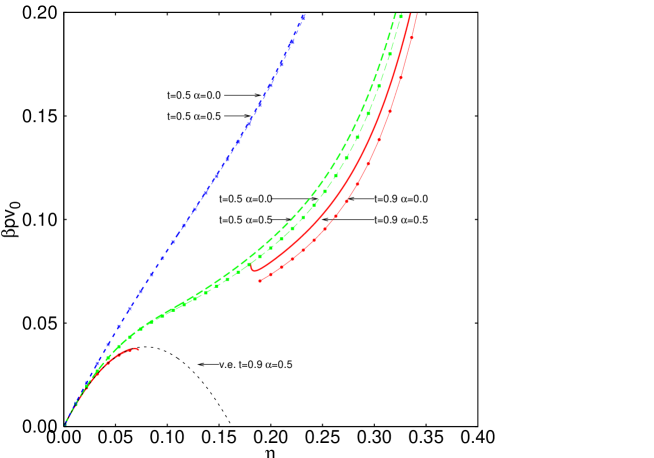
Figure 5: (Color online) A plot of $\beta pv_{0}$ versus the packing fraction $\eta$ for four different values of $t=1/(12\tau),$ with ($\alpha=1/2$) and without ($\alpha=0$) the anisotropic contribution, using the virial route to the pressure. The 3rd order virial expansion is also added (v.e.) in the most relevan case $t=0.9$ and $\alpha=0.5$ for comparison. The part of the lines which are not shown correspond to a loss of solutions.

For given $t,\eta$, one can calculate $y_{0}(\sigma)$, $y_{D}(\sigma)$, $Y_{0}^{\prime}(\sigma)$ and $Y_{D}^{\prime}(\sigma)$ analytically using expressions from Ref. I. However, $Y_{0}^{\prime}(\sigma)$ and $Y_{D}^{\prime}(\sigma)$ require some care, since space derivative and sticky limit do not commute Baxter68 . So from Eq. (26) one finds the virial pressure. The corresponding results are collected in Fig. 5 for different values of $t$, at both $\alpha=0$ (isotropic case) and $\alpha=1/2$ (with the anisotropic contribution included). A comparison with the virial expansion up to the third virial coefficient is also added in the case $t=0.9$ and $\alpha=1/2$.

In agreement with the previous structural findings, we find a dependence on the anisotropy. This is very small for $t\leq 0.5$ but increasingly appreciable for larger values of the adhesion strength $t$. In Fig. 5 one clearly sees that the pression increases by roughly $10\%$ on going from $\alpha=0$ (no anisotropy) to $\alpha=0.5$ (maximum anisotropy) for $t=0.9$ and $\eta\geq 0.2$.

Despite the strong differences with the pure dipolar case, it proves instructive to get some insight into the competition between the tendency to condensation on the one hand and to chaining on the other hand, by applying to the present model the arguments put forward by Tlusty and Safran Tlusty00 in the dipolar case. These authors devised a phenomenological theory, where the two above-mentioned tendencies are represented by the concentrations of  ‘junctions’ and ‘ends’, respectively (see Ref. Tlusty00, ). We have closely followed their arguments to derive the critical parameters $\tau_{c}$ and $\eta_{c}$ of the present model in terms of the energies $\epsilon_{1}$, $\epsilon_{3}$ of ends and junctions respectively. One finds Tlusty00

$$\tau_{c}=\frac{\epsilon_{1}-3\epsilon_{3}}{3\ln 3-2\ln 2}~{},\text{ \ \ \ \ \ \ \ \ \ \ \ }\ln\eta_{c}=-\frac{\epsilon_{1}(2\ln 3-\ln 2)-\epsilon_{3}\ln 2}{\epsilon_{1}-3\epsilon_{3}}~{}.$$ (27)

which coincides with the results of Ref. Tlusty00, . Matching this critical values with the one of the isotropic adhesive spheres of Miller and Frenkel Miller04 , $\tau_{c}=0.1133$ and $\eta_{c}=0.266$, we find $\epsilon_{1}=0.186$ and $\epsilon_{3}=-0.0102$ (the value $\epsilon_{3}<0$ means that junctions are enhanced with respect to ends, once more favoring condensation). In our results the number of ends $\rho_{1}$ and junctions $\rho_{3}$ turn out to be equal ($\rho_{1}=\rho_{3}$) at the critical point, which is thus a point of connectivity transition in the system. Fig. 6 depicts the coexistence line, which does not display the re-entrance characteristic of the pure dipolar case (compare with Fig. 2 of Ref. Tlusty00, ). This is in complete agreement with the remark by Tlusty and Safran that the addition of an isotropic short-range attraction  – such as the case of the present model – reports the curve to its characteristic parabolic shape (see also Fig. 3 of Ref. Tlusty00, ). This is also consistent with very recent numerical simulation results Ganzenmuller09 ; Martin09 showing that the addition of a very weak isotropic attraction to the dipolar HS potential makes the condensation transition easily observable.

In summary, we have studied structural and thermophysical properties of a particular hard-core fluid where the attractive part of the potential includes an anisotropy of dipolar form infinitesimally short and infinitely strong.

Any two molecules of the fluid interact only at contact with a potential having, in addition to an adhesive isotropic part of the Baxter type, an additional adhesive term, whose intensity depends upon the mutual orientation of the two particles in a dipolar fashion.

Our potential belongs to a class of simple anisotropic models that have recently attracted considerable interest in connection with aggregation phenomena in colloidal fluids, polymers and globular proteins, because of their possible experimental relevance for self-assembling materials and biological viruses.

The extremely short-range nature of this peculiar dipolar interaction strongly contrasts with the long-range nature of the dipolar hard sphere model. In the latter case, the formation of chains and long anisotropic agglomerates significantly affects the possibility of a gas-liquid transition. Using a simplified treatment of the angular part, based upon a first-order expansion in angular invariants so to allow an almost fully analytical solution, we have shown that only the local (first few) coordination shells are affected by the anisotropy. This is due to the fact that the the orientationally dependent part of the potential has a relatively weak strength with respect to the isotropic attractive term, as forced by the particular choice of the potential associated with the $0\leq\alpha\leq 1/2$ limits. As a result, all structural and thermodynamical properties are only mildly affected by the anisotropic adhesion.

Nonetheless, the competition of the two adhesive terms (the isotropic and the anisotropic ones) gives rise to an anisotropic local ordering within each (almost isotropic) molecular agglomerate consisting of short chains of molecules with parallel head-to-tail orientation, ‘glued’ to similar chains globally oriented in the opposite direction, thus giving an antiparallel alignment for particles belonging to two adjacent chains.

It would be interesting to contrast the present results with more realistic models incorporating a competition between an isotropic and anisotropic short range interactions, such as for instance Stockmayer fluids Leeuwen93 , dipolar Yukawa HS fluids Slazai99 or combination of dipolar and square-well potentials Martin09 .

In spite of its simplicity, the results of the present work suggest that, in the presence of dipolar-like anisotropy, one can continuously tune from situations only affecting the local ordering (such as in the case presented here) to situations where this effect is much more global (such as the real dipolar case), by simply adjusting the range of interaction.

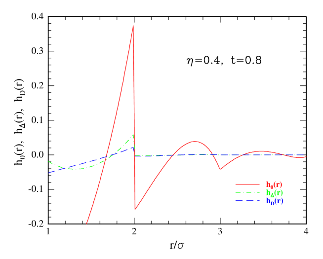
Figure 2: (Color online) The three components $h_{0}(r)$, $h_{\Delta}(r)$ and $h_{D}(r)$ of the molecular total correlation function, for $\alpha=1/2$, $\eta=0.4$, and $t=0.8$. At $r<\sigma$ one has $h_{0}(r)=-1$, $h_{\Delta}(r)=h_{D}(r)=0$.

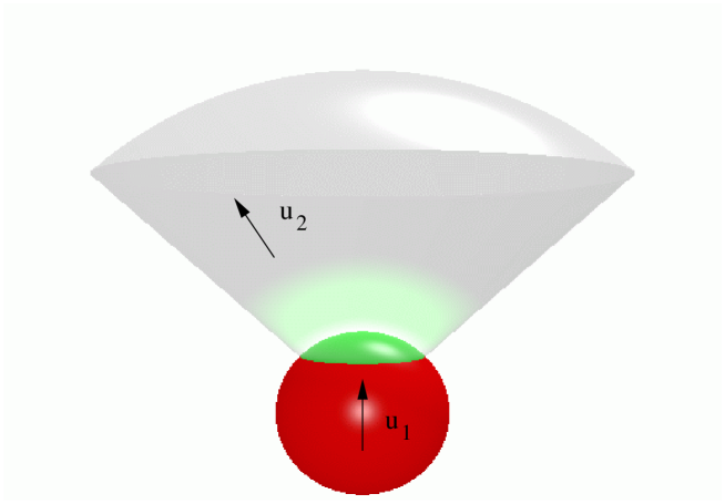
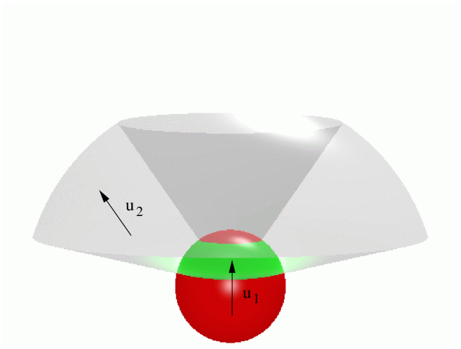
Figure 3: (Color online) Schematic representation of the volume $V_{AB}$ (included in the shading area) in two different situations: (top panel) $\theta_{A}=0$ giving the contribution from the forward region, and (bottom panel ) $\theta_{A}\neq\theta_{B}\neq 0$ giving information on the lateral adjacent region.

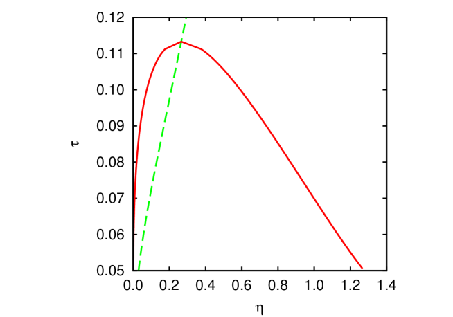
Figure 6: (Color online) Phase diagram of our dipolar-like sticky hard spheres, calculated for defect energies $\epsilon_{1}=0.186$ and $\epsilon_{3}=-0.0102$. At the critical point the binodal curve (continuous line) and the connectivity transition (dashed curve) meet. The line denote the end-rich “gas” with the junction-rich “liquid”.

- (1) E. Zaccarelli, C. Valeriani, E. Sanz, W.C.K. Poon, M.E. Cates, and P. N. Pusey, Phys. Rev. Lett. 103, 135704 (2009)
- (2) E. Zaccarelli, J. Phys.: Condensed Matter 19, 323101 (2007).
- (3) A. Yethiraj and A. van Blaaderen, Nature 421, 513 (2003).
- (4) P.J. Lu, E. Zaccarelli, F. Ciulla, A. B. Schofield, F. Sciortino and D. Weitz, Nature 453, 499 (2008).
- (5) N. Kern, and D. Frenkel, J. Chem. Phys. 118, 9882 (2003).
- (6) R. Fantoni, D. Gazzillo, A. Giacometti, M.A. Miller and G. Pastore, J. Chem. Phys. 127, 234507 (2007); A. Giacometti, F. Lado, J. Largo, G. Pastore and F. Sciortino, J. Chem. Phys. 131, 174114 (2009)
- (7) H. Liu, S. K. Kumar and F. Sciortino, J. Chem. Phys. 127, 084902 (2007).
- (8) G. Foffi and F. Sciortino, J. Phys. Chem. B 111, 9702 (2007).
- (9) E. Bianchi, P. Tartaglia, E. Zaccarelli and F. Sciortino, J. Chem. Phys. 128, 144504 (2008).
- (10) C. Gögelein, G. Nägele, R. Tuinier, T. Gibaud, A. Strader and P. Schurtenberger, J. Chem. Phys. 129, 085102 (2008).
- (11) J.M. Tavares, P.I.C. Teixeira, and M.M. Telo de Gama, Mol. Phys. 107, 453 (2009).
- (12) M. S. Wertheim, J. Chem. Phys. 55, 4291 (1971).
- (13) T. Tlusty and S.A. Safran, Science 290, 1328 (2000).
- (14) P.J. Camp, J.C. Shelley and G.N. Patey, Phys. Rev. Lett. 84, 115 (2000).
- (15) G. Ganzenmüller and P.J. Camp, J. Chem. Phys. 126, 191104 (2007).
- (16) R. J. Baxter, J. Chem. Phys. 49, 2770 (1968).
- (17) D. Gazzillo, R. Fantoni, and A. Giacometti, Phys. Rev. E 78, 021201, (2008).
- (18) G. Jackson, W. G. Chapman, and K. E. Gubbins, Mol. Phys. 65, 1 (1988).
- (19) R. P. Sear, J. Chem. Phys. 111, 4800 (1999).
- (20) D. Ghonasgi, and W. G. Chapman, J. Chem. Phys. 102, 2585 (1995).
- (21) E. Mileva, and G. T. Evans, J. Chem. Phys. 113, 3766 (2000).
- (22) Z. Zhang, A. S. Keys, T. Chen, and S. C. Glotzer, Langmuir, 21, 11547 (2005).
- (23) C. G. Gray, and K. E. Gubbins, Theory of Molecular Fluids, Vol. I, Appendix 3E (Clarendon Press, Oxford, 1984).
- (24) M. Miller and D. Frenkel, J. Chem. Phys. 121, 535 (2004).
- (25) G. Ganzenmüller, G.N. Patey, and P.J. Camp, Mol. Phys. 107, 403 (2009).
- (26) M. Martín-Betancourt, J.M. Romero-Enrique, and L.F. Rull, Mol. Phys. 107, 563 (2009).
- (27) M.E. van Leeuwen, and B. Smit, Phys. Rev. Lett. 71, 3991 (1993).
- (28) I. Slazai, D. Henderson, D. Boda, and K.Y. Chan, J. Chem. Phys. 119, 337 (1999).