EvoL: The new Padova T-SPH parallel code for cosmological simulations - I. Basic code: gravity and hydrodynamics

Abstract

Context. We present EvoL, the new release of the Padova N-body code for cosmological simulations of galaxy formation and evolution. In this paper, the basic Tree + SPH code is presented and analysed, together with an overview on the software architectures.

Aims. EvoL is a flexible parallel Fortran95 code, specifically designed for simulations of cosmological structure formation on cluster, galactic and sub-galactic scales.

Methods. EvoL is a fully Lagrangian self-adaptive code, based on the classical Oct-tree by Barnes & Hut (1986) and on the Smoothed Particle Hydrodynamics algorithm (SPH, Lucy 1977). It includes special features such as adaptive softening lengths with correcting extra-terms, and modern formulations of SPH and artificial viscosity. It is designed to be run in parallel on multiple CPUs to optimize the performance and save computational time.

Results. We describe the code in detail, and present the results of a number of standard hydrodynamical tests.

1 Introduction

The importance of numerical simulations in modern science is constantly growing, because of the complexity, the multi-scaling properties, and the non-linearity of many physical phenomena. When analytical predictions are not possible, we are forced to compute the evolution of physical systems numerically. Typical examples in astrophysical context are the problems of structure and galaxy formation and evolution. Over the past two decades, thanks to highly sophisticated cosmological and galaxy-sized numerical simulations a number of issues concerning the formation of cosmic systems and their evolution along the history of the Universe have been clarified. However, an equivalent number of new questions have been raised, so that complete understanding of how galaxies and clusters formed and evolved along the Hubble time is still out of our reach. This is especially true at the light of many recent observations that often appear at odds with well established theories (see for instance the long debated question of the monolithic versus hierarchical mechanism of galaxy formation and their many variants) and to require new theoretical scenarios able to match the observational data.

To this aim, more and more accurate and detailed numerical simulations are still needed. They indeed are the best tool to our disposal to investigate such complex phenomena as the formation and evolution of galaxies within a consistent cosmological context. A number of astrophysical codes for galaxy-sized and cosmological simulations are freely and publicly available. They display a huge range of options and functions; each of them is best suited for a set of particular problems and experiments, and may suffer one or more drawbacks. Among the best known, we recall Flash (Fryxell et al. 2000), Gadget (Springel et al. 2001) and its second release Gadget2 (Springel 2005), Gasoline (Wadsley et al. 2004), Hydra (Couchman et al. 1995), Enzo (Norman et al. 2007), and Vine (Wetzstein et al. 2008).

EvoL is the new release of the Padova N-body code (Pd-Tsph, Carraro et al. 1998; Lia et al. 2002; Merlin & Chiosi 2007). It is a flexible, fully Lagrangian, parallel, and self-adaptive N-body code, written in Fortran95 in a straightforward and user-friendly format.

EvoL describes the dynamical evolution of a system of interacting discrete masses (particles) moving under the mutual gravitational forces and/or the gravitational action of external bodies, plus, when appropriate, under mutual hydrodynamical interactions. Such particles can represent real discrete bodies or a fluid contained in volume elements of suitable size. A numerical simulation of a physical system follows the temporal evolution of it using small but finite time-steps to approximate the equations of motion to a finite-differences problem. In the Lagrangian description, no reference grid is superposed to the volume under consideration, while the particles move under their mutual (or external) interactions. Each particles carries a mass, a position, a velocity, plus (when necessary) a list of physical features such as density, temperature, chemical composition, etc.

To simulate the dynamical evolution of a region of the Universe, one has to properly model the main different material components, namely Dark Matter, Gas, and Stars), representing them with different species of particles. Moreover, a physically robust model for the fundamental interactions (in addition to gravity) is required, at the various scales of interest. Finally, a suitable cosmological framework is necessary, together with a coherent setting of the boundary conditions and with an efficient algorithm to follow the temporal evolution of the system. EvoL is designed to respond to all of these requirements, improving upon the previous versions of the Padova Tree-SPH code under many aspects. In the following sections, the main features of EvoL are presented in detail, together with a review of some general considerations about the adopted algorithms whenever appropriate.

This paper presents the basic features of the code; namely, the Tree-SPH (i.e. Oct-Tree plus Smoothing Particle Hydrodynamics) formalism, its implementation in the parallel architecture of the code, and the results of a number of classic hydrodynamic tests. The non-standard algorithms (e.g. radiative cooling functions, chemical evolution, star formation, energy feedback) will be presented in a following companion paper (Merlin et al. 2009, in preparation).

The plan of the paper is as follows. In Sect. 2 we describe the aspects of the code related to the gravitational interaction. In Sect. 3 we deal with the hydrodynamical treatment of fluids and its approximation in the SPH language. Sect. 4 illustrates some aspects related to the integration technique, such as the time steps, the periodic boundary conditions, and the parallelization of the code. Sect. 5 contains and discusses numerous tests aimed at assessing the performance of the code. Sect.6 summarizes some concluding remarks. Finally, Appendices A and B contains some technical details related the N-dimensional spline kernel (Appendix A) and the equations of motion and energy conservation (Appendix B).

2 Description of the code: Gravity

Gravity is the leading force behind the formation of cosmic structures, on many scales of interest, from galaxy clusters down to individual stars and planets. Classical gravitation is a well understood interaction. As long as General Relativity, Particle Physics or exotic treatments such as Modified Dynamics are not considered , it is described by Newton’s law of universal gravitation:

$$\@vec{F}_{ij}=G\frac{m_{i}m_{j}}{|\@vec{r}_{j}-\@vec{r}_{i}|^{3}}(\@vec{r}_{j}-\@vec{r}_{i}),$$ (1)

where $G$ is the gravitational constant. Given a density field $\rho(\@vec{r})$, the gravitational potential $\Phi$ is obtained via Poisson equation:

$$\nabla^{2}\Phi(\@vec{r})=4\pi G\rho(\@vec{r}),$$ (2)

and $\@vec{F}_{ij}=\nabla\Phi(\@vec{r})$.

The gravitational force exerted on a given body (i.e., particle) by the whole system of bodies within a simulation can be obtained by the vectorial summation of all the particles’ contributions (without considering, for the moment, the action of the infinite region external to the computational volume; this can indeed be taken into account using periodic boundary conditions, see Sect. 4.3). This is simply the straightforward application of Eq. 1. Anyway, in practice this approach is not efficient, and may also lead to artificial divergences, as explained in the following Sections.

2.1 Softening of the gravitational force

Close encounters between particles can cause numerical errors, essentially because of the time and mass resolution limits. Moreover, when dealing with continuous fluids rather than with single, isolated objects, one tries to solve Eq. 2 rather than Eq. 1, and must therefore try to model a smooth density field given a distribution of particles with mass. In addition, dense clumps of particles may also steal large amounts of computational time. To cope with all these issues, it is common practice to soften the gravitational force between close pairs of bodies: if the distance between two particles becomes smaller than a suitable softening length $\epsilon$, the force exerted on each body is corrected and progressively reduced to zero with decreasing distance.

Different forms of the force softening function can be used. A possible expression is given by the following formula:

$$\frac{F(\@vec{r},\epsilon)}{Gm_{i}}=m_{j}\frac{\@vec{r}}{|\@vec{r}|}\times$$ (3)

$$\begin{cases}1/\epsilon^{2}[\frac{4}{3}u-\frac{6}{5}u^{3}+\frac{1}{2}u^{4}]&\text{if $0\leq u<1$,}\\ 1/\epsilon^{2}[\frac{8}{3}u-3u^{2}+\frac{6}{5}u^{3}-\frac{1}{6}u^{4}-\frac{1}{15u^{2}}]&\text{if $1\leq u<2$,}\\ 1/|\@vec{r}|^{2}&\text{if $u\geq 2$,}\end{cases}$$

where $\@vec{r}$ is the distance between particles $i$ and $j$, and $u\equiv|\@vec{r}|/\epsilon$. This expression for the force softening corresponds (via the Poisson equation) to a density distribution kernel function proposed by Monaghan & Lattanzio (1985) and widely adopted in Smoothed Particles Hydrodynamics algorithms (see Sect. 3) :

$$W(r,\epsilon)=\frac{1}{\pi h^{3}}\times\begin{cases}1-\frac{3}{2}u^{2}+\frac{3}{4}u^{3}&\text{if $0\leq u<1$,}\\ \frac{1}{4}(2-u)^{3}&\text{if $1\leq u<2$,}\\ 0&\text{if $u\geq 2$.}\end{cases}$$ (4)

Note that in Eq. 2.1 the softening length $\epsilon$ is assumed to be the same for the two particles $i$ and $j$. In the more general situation in which each particle carries its own $\epsilon$, a symmetrisation is needed to ensure energy and momentum conservation: this can be achieved either using $\epsilon=\bar{\epsilon_{ij}}=(\epsilon_{i}+\epsilon_{j})/2$, or by symmetrizing the softened force after computing it with the two different values $\epsilon_{i}$ and $\epsilon_{j}$.

The softening lengths can be fixed in space and time, or may be let vary with local conditions. If the softening length is kept constant, the choice of its numerical value is of primary importance: for too small a softening length it will result in noisy force estimates, while for too large a value it will systematically bias the force in an unphysical manner (Merritt 1996; Romeo 1998; Athanassoula et al. 2000; Price & Monaghan 2007, and see also Sect. 5.9). Unfortunately, the “optimal” value for the softening length depends on the particular system being simulated, and in general it is not known a priori. A standard solution is to assign to each particle a softening length proportional to its mass, keeping it fixed throughout the whole simulation, or letting it vary with time, or redshift, if a cosmological background is included. A clear advantage of keeping $\epsilon$ fixed in space is that energy is naturally conserved, but on the other hand the smallest resolvable length scale is fixed at the beginning of the simulation and remains the same in the whole spatial domain independently of the real evolution of the density field. A collapsing or expanding body may quickly reach a size where the flow is dominated by the softening in one region, while in another the flow may become unphysically point-like.

Obviously, the accuracy can be greatly improved if $\epsilon$ is let vary according to the local particle number density (see e.g. Dehnen 2001). Moreover, in principle, if particles in a simulation are used to sample a continuous fluid (whose physics is determined by the Navier-Stokes or the Boltzmann equations) the properties of such points should always change accordingly to the local properties of the fluid they are sampling, to optimize the self-adaptive nature of Lagrangian methods. On the other hand, if particles represent discrete objects (single stars, or galaxies in a cluster, etc.), their softening lengths might perhaps be considered an intrinsic property of such objects and may be kept constant, depending on their mass and not on the local density of particles. In cosmological and galaxy-sized simulations, gas and Dark Matter particles are point-masses sampling the underlying density field, and stellar particles represent clusters of thousands of stars prone to the gravitational action of the nearby distribution of matter; thus a fully adaptive approach seems to be adequate to describe the evolution of these fluids. However, it can be easily shown that simply letting $\epsilon$ change freely would result in a poor conservation of global energy and momentum, even if in some cases the errors could be small (see e.g. Price & Monaghan 2007; Wetzstein et al. 2008).

To cope with this, EvoL allows for the adaptive evolution of individual softening lengths, but includes in the equations of motion of particles self-consistent correcting additional terms. Such terms can be derived (see Price & Monaghan 2007) starting from an analysis of the Lagrangian describing a self-gravitating, softened, collisionless system of $N$ particles, which is given by

$$L=\sum_{i=1}^{N}m_{i}\left(\frac{1}{2}v_{i}^{2}-\Phi_{i}\right),$$ (5)

where $\Phi$ is the gravitational potential of the $i$-th particle,

$$\Phi(\@vec{r}_{i})=-G\sum_{j=1}^{N}m_{j}\phi(|\@vec{r}_{ij}|,\epsilon_{i}),$$ (6)

and $\phi$ is a softening kernel ($\@vec{r}_{ij}=\@vec{r}_{i}-\@vec{r}_{j}$). Assuming a density distribution described by the standard spline kernel Eq. 4, the latter becomes

$$\phi(\@vec{r},\epsilon)=$$ (7)

$$\begin{cases}1/\epsilon[\frac{2}{3}u^{2}-\frac{3}{10}u^{4}+\frac{1}{10}u^{5}-\frac{7}{5}]&\text{if $0\leq u<1$,}\\ 1/\epsilon[\frac{4}{3}u^{2}-u^{3}+\frac{3}{10}u^{4}-\frac{1}{30}u^{5}-\frac{8}{5}+\frac{1}{15u}]&\text{if $1\leq u<2$,}\\ -1/|\@vec{r}|&\text{if $u\geq 2$,}\end{cases}$$

where again $u\equiv|\@vec{r}|/\epsilon$. Note that the force softening, Eq. 2.1, is obtained taking the spatial derivative of Eq. 2.1.

The equations of motion are obtained from the Euler-Lagrange equations,

$$\frac{d}{dt}\left(\frac{\partial L}{\partial\@vec{v}_{i}}\right)-\frac{\partial L}{\partial\@vec{r}_{i}}=0,$$ (8)

which give

$$m_{i}\frac{d\@vec{v}_{i}}{dt}=\frac{\partial L}{\partial\@vec{r}_{i}}.$$ (9)

The gravitational part of the Lagrangian is

$$L_{grav} = -\sum_{j=1}^{N}m_{j}\Phi_{j}=$$

$$-\frac{G}{2}\sum_{j}\sum_{k}m_{j}m_{k}\phi_{jk}(\epsilon_{j})$$

where for the sake of clarity $\phi_{ij}(\epsilon_{i})=\phi(|\@vec{r}_{ij}|,\epsilon_{i})$; swapping indices, the partial derivative $\partial L_{grav}/\partial\@vec{r}_{i}$ results

$$\frac{\partial L_{grav}}{\partial\@vec{r}_{i}}=$$ (11)

$$-\frac{G}{2}\sum_{j}\sum_{k}m_{j}m_{k}\left[\frac{\partial\phi_{jk}(\epsilon_{j})}{\partial|r_{jk}|}|_{\epsilon}\frac{\partial|r_{jk}|}{\partial\@vec{r}_{i}}+\frac{\partial\phi_{jk}(\epsilon_{j})}{\partial\epsilon_{j}}|_{r}\frac{\partial\epsilon_{j}}{\partial\@vec{r}_{i}}\right],$$

where

$$\frac{\partial|r_{jk}|}{\partial\@vec{r}_{i}}=\frac{\@vec{r}_{j}-\@vec{r}_{k}}{|\@vec{r}_{j}-\@vec{r}_{k}|}(\delta_{ji}-\delta_{ki}).$$ (12)

To obtain the required terms in the second addend on the right part of Eq. 2.1, the softening length must be related to the particle coordinates so that $\epsilon=\epsilon(n)$, where $n$ is the number density of particles at particle $i$ location. To this aim, one can start from the general interpolation rule that any function of coordinates $A(\@vec{r})$ can be expressed in terms of its values at a disordered set of points, and the integral interpolating the function $A(\@vec{r})$ can be defined by

$$A_{int}(\@vec{r})=\int{A(\@vec{r}^{\prime})W(\@vec{r}-\@vec{r}^{\prime},\epsilon)\@vec{dr^{\prime}}},$$ (13)

where $W$ is the density kernel Eq. 4. This is the same rule at the basis of the SPH scheme (see Sect. 3) .

Approximating the integral to a summation over particles for practice purposes, one obtains

$$A_{sum}(\@vec{r}_{i})=A_{i}=\sum_{j}{\frac{A_{j}}{n_{j}}W(\@vec{r}_{ij},\epsilon_{i})},$$ (14)

where $i$ marks the “active” particle that lays at the position at which the function is being evaluated, and $j$ are its neighbouring particles (or simply neighbours). The error by doing so depends on the disorder of particles and is in general $O(h^{2})$ (Monaghan 1992). Thus,

$$n_{i}=\sum_{j}W(|\@vec{r}_{ij}|,\epsilon_{i}),$$ (15)

where it has been put $A=n$; so, there is no need to know in advance the value of the density of neighbouring particles to compute the density of the active one.

To link $\epsilon$ and $n$, a safe prescription is to use

$$\epsilon_{i}=\eta\left(\frac{1}{n_{i}}\right)^{1/3},$$ (16)

where $\eta$ is a dimensionless parameter. With this law, the weighted number of particles within a softening sphere is tentatively held constant, i.e.

$$\frac{4}{3}(2\epsilon_{i})^{3}n_{i}=N_{nei,id},$$ (17)

with $N_{nei,id}{3}\pi(2\eta)^{3}$. Numerical experiments have shown that a safe choice is $1.2\leq\eta\leq 1.5$, corresponding to $60\leq N_{nei,id}\leq 110$ (Price & Monaghan 2007).

The term needed in Eq. 2.1 is

$$\frac{\partial\epsilon_{j}}{\partial\@vec{r}_{i}}=\frac{\partial\epsilon_{j}}{\partial n_{j}}\frac{\partial n_{j}}{\partial\@vec{r}_{i}}.$$ (18)

The first factor is given by the derivative of Eq. 16,

$$\frac{\partial\epsilon_{j}}{\partial n_{j}}=-\frac{\epsilon_{j}}{3n_{j}},$$ (19)

whereas the second factor is the spatial derivative of Eq. 15, which results:

$$\frac{\partial n_{j}}{\partial\@vec{r}_{i}}=\frac{1}{\Upsilon_{j}}\sum_{p}\frac{\partial W_{jp}(\epsilon_{j})}{\partial\@vec{r}_{i}}(\delta_{ij}-\delta_{ip}),$$ (20)

where it was defined

$$\Upsilon_{i}=\left[1-\frac{\partial\epsilon_{i}}{\partial n_{i}}\sum_{j}\frac{\partial W_{ij}(\epsilon_{i})}{\partial\epsilon_{i}}\right].$$ (21)

Rearranging and putting $G\equiv 1$, one finally finds

$$\frac{\partial L_{grav}}{\partial\@vec{r}_{i}} =$$

$$-m_{i}\sum_{j}m_{j}\left[\frac{\phi_{ij}^{\prime}(\epsilon_{i})+\phi_{ij}^{\prime}(\epsilon_{j})}{2}\right]\frac{\@vec{r}_{i}-\@vec{r}_{j}}{|\@vec{r}_{i}-\@vec{r}_{j}|}$$

$$-m_{i}\sum_{j}m_{j}\frac{1}{2}\left[\frac{\xi_{i}}{\Upsilon_{i}}\frac{\partial W_{ij}(\epsilon_{i})}{\partial\@vec{r}_{i}}+\frac{\xi_{j}}{\Upsilon_{j}}\frac{\partial W_{ij}(\epsilon_{i})}{\partial\@vec{r}_{j}}\right],$$

where

$$\xi_{i}=\frac{\partial\epsilon_{i}}{\partial n_{i}}\sum_{j}\frac{\partial\phi_{ij}(\epsilon_{i})}{\partial\epsilon_{i}}.$$ (23)

The $\partial\phi/\partial\epsilon$ terms used in Eq. 23 can be tabulated together with the other kernel functions:

$$\frac{\partial\phi}{\partial\epsilon}=$$ (24)

$$\begin{cases}1/\epsilon^{2}[-2u^{2}+\frac{3}{2}u^{4}-\frac{3}{5}u^{5}+\frac{7}{5}]&\text{if $0\leq u<1$,}\\ 1/\epsilon^{2}[-4u^{2}+4u^{3}+\frac{3}{2}u^{4}+\frac{1}{5}u^{5}+\frac{8}{5}]&\text{if $1\leq u<2$,}\\ 0&\text{if $u\geq 2$,}\end{cases}$$

where, as usual, $u\equiv|\@vec{r}|/\epsilon$. Finally, the $\partial W/\partial\@vec{r}$ and $\partial W/\partial\epsilon$ terms are easily obtained deriving the explicit expression of $W(|\@vec{r}|,\epsilon)$.

In Eq. 22 (and Eq. 12), the first term is the classical gravitational interaction, whereas the second term is a new, extra-term which restores energy conservation for varying softening lengths. Since $\xi$ is defined as a negative quantity for positive kernels, this term acts as a negative pressure, increasing the gravitational force. To obtain the $\xi$ and $\Upsilon$ correcting terms, each particle $i$ must perform a loop over the other particles, summing the contributions from the ones that satisfy the criterion $|\@vec{r}_{ij}|\leq 2\times\max(\epsilon_{i},\epsilon_{j})$ .

The relation between $\epsilon$ and $n$, defined by Eq. 16, leads to a non-linear equation which can be solved self-consistently for each particle. Price & Monaghan (2007) proposed an iterative method in which, beginning from a starting guess for both $n$ and $\epsilon$, the solution of the equation

$$f(\epsilon)=|n_{i}(\epsilon_{i})-n_{sum,i}(\epsilon_{i})|=0,$$ (25)

where $n_{sum,i}(\epsilon_{i})$ is the mass density computed via summation over neighbouring particles (Eq. 15) and $n_{i}(\epsilon_{i})$ is the density obtained from Eq. 16, is searched by means of an iterative procedure, that can be solved adopting a classical bisection scheme, or more efficient routines such as the Newton-Raphson method. In this case, a loop is iterated until $|\epsilon_{i,new}-\epsilon_{i}|/\epsilon_{i,init}<\gamma_{TOL}$, where $\gamma_{TOL}$ is a tolerance parameter $\sim 10^{-2}-10^{-3}$, $\epsilon_{i,init}$ is the value of $\epsilon$ for the particle $i$ at the beginning of the procedure, $\epsilon_{i}$ is its current value, and $\epsilon_{i,new}=\epsilon_{i}-f(\epsilon_{i})/f^{\prime}(\epsilon_{i})$; the derivative of Eq. 25 is given by

$$f^{\prime}(\epsilon_{i})=\frac{\partial n_{i}}{\partial\epsilon_{i}}-\sum_{j}m_{j}\frac{\partial W_{ij}(\epsilon_{i})}{\partial\epsilon_{i}}=-\frac{3n_{i}}{\epsilon_{i}}\Upsilon_{i}.$$ (26)

To increase the efficiency of this process, a predicted value for both $\epsilon$ and $n$ can be obtained at the beginning of each time-step using a discretized formulation of the Lagrangian continuity equation,

$$\frac{dn}{dt}=-n(\nabla\cdot\@vec{v}).$$ (27)

Such formulation can be obtained taking the time derivative of Eq. 15, which results

$$\frac{dn_{i}}{dt}=\frac{1}{\Upsilon_{i}}\sum_{j}(\@vec{v}_{i}-\@vec{v}_{j})\cdot\nabla_{i}W(\@vec{r}_{ij},\epsilon),$$ (28)

while

$$\frac{d\epsilon_{i}}{dt}=\frac{\partial\epsilon_{i}}{\partial n_{i}}\frac{dn_{i}}{dt}.$$ (29)

Combining Eq. 28 with Eq. 27, one can also see that the velocity divergence at $i$ particle location is given by

$$\nabla\cdot\@vec{v}_{i}=-\frac{1}{n_{i}\Upsilon_{i}}\sum_{j}(\@vec{v}_{i}-\@vec{v}_{j})\cdot\nabla_{i}W(\@vec{r}_{ij},\epsilon).$$ (30)

The adoption of this adaptive softening length formalism, with the correcting extra-terms in the equation of motion, results in small errors, always comparable in magnitude to the ones found with the “optimal” $\epsilon$ (see Price & Monaghan 2007, their Figs. 2, 3 and 4).

At the beginning of a simulation, the user can select whether he/she prefers to adopt the constant or the adaptive softening lengths formalism, switching on or off a suitable flag.

2.2 Hierarchical oct-tree structure

A direct summation of the contribution of all particles should in principle be performed for each particle at each time-step to correctly compute the gravitational interaction, leading to a computational cost increasing with $N^{2}$ ($N$ being the number of particles). A convenient alternative to this unpractical approach are the so-called tree structures, in which particles are arranged in a hierarchy of groups or “cells”. In this way, when the force on a particle is computed, the contribution by distant groups of bodies can be approximated by their lowest multipole moments, reducing the computational cost to evaluate the total force to $O(NlogN)$. In the classical Barnes & Hut (1986) scheme, the computational spatial domain is hierarchically partitioned into a sequence of cubes, where each cube contains eight siblings, each with half the side-length of the parent cube. These cubes form the nodes of an oct-tree structure. The tree is constructed such that each node (cube) contains either a desired number of particles (usually one, or one per particles type - Dark Matter, gas, stars), or is progenitor of further nodes, in which case the node carries the monopole and quadrupole moments of all the particles that lie inside the cube. The force computation then proceeds by walking along the tree, and summing up the appropriate force contributions from tree nodes. In the standard tree walk, the global gravitational force exerted by a node of linear size $l$ on a particle $i$ is considered only if $r>l/\theta$, where $r$ is the distance of the node from the active particle and $\theta$ is an accuracy parameter (usually $\leq 1$): if a node fulfills the criterion, the tree walk along this branch can be terminated, otherwise it is “opened”, and the walk is continued with all its siblings. The contribution from individual particles is thus considered only when they are sufficiently close to the particle $i$.

To cope with some problems pointed out by Salmon & Warren (1994) about the worst-case behaviour of this standard criterion for commonly employed opening angles, Dubinski (1996) introduced the simple modification

$$r>l/\theta+\delta,$$ (31)

where the $\delta$ is the distance of the geometric center of a cell to its center of mass. This provides protection against pathological cases where the center of mass lies close to an edge of a cell.

In practice, this whole scheme only includes the monopole moment of the force exerted by distant groups of particles. Higher orders can be included, and the common practice is to include the quadrupole moment corrections (EvoL indeed includes them). Still higher multipole orders would result in a worst performance without significant gains in computational accuracy (McMillan & Aarseth 1993).

Note that if one has the total mass, the center of mass, and the weighted average softening length of a node of the oct-tree structure, the softened expression of the gravitational force can be straightforwardly computed treating the cell as a single particle if the opening criterion is fulfilled but the cell is still sufficiently near for the force to need to be softened.

As first suggested by Hernquist & Katz (1989), the tree structure can be also used to obtain the individual lists of neighbours for each body. At each time step each (active) particle can build its list of interacting neighbouring particles while walking the tree and opening only sufficiently nearby cells, until nearby bodies are reached and linked.

3 Description of the code: Hydrodynamics

Astrophysical gaseous plasmas can generally be reasonably approximated to highly compressible, unviscous fluids, in which anyway a fundamental role is played by violent phenomena such as strong shocks, high energy point-like explosions and/or supersonic turbulent motions. EvoL follows the basic gas physics by means of the Smoothed Particles Hydrodynamics (SPH, Lucy 1977; Monaghan 1992), in a modern formulation based on the review by Rosswog (2009), to which the reader is referred for details. Anyway, some different features are present in our implementation and we summarize them in the following, along with a short review of the whole SPH algorithm.

To model fluid hydrodynamics by means of a discrete description of a continuous the fluid, in the SPH approach the properties of single particles are smoothed in real space through the kernel function $W$, and thus weighted by the contributions of neighbouring particles. In this way, the physical properties of each point in real space can be obtained by the summation over particles of their individual, discrete properties. Note that, on the contrary of what happens when softening the gravitational force (which is gradually reduced to zero within the softening sphere), in this case the smoothing sphere is the only “active” region, and only particles inside this region contribute to the computation of the local properties of the central particle.

Starting again from the interpolation rule described in Sect. 2.1, but replacing the softening length $\epsilon$ by a suitable smoothing length $h$, the integral interpolating the function $A(\@vec{r})$ becomes

$$A_{i}(\@vec{r})=\int{A(\@vec{r}^{\prime})W(\@vec{r}-\@vec{r}^{\prime},h)\@vec{dr^{\prime}}},$$ (32)

(the kernel function $W$ can be the density kernel Eq. 4).

The relative discrete approximation becomes

$$A_{s}(\@vec{r}_{i})=\sum_{j}{\frac{A_{j}}{\rho_{j}}m_{j}W(\@vec{r}_{i}-\@vec{r}_{j},h_{i})},$$ (33)

and the physical density of any SPH particle can be computed as

$$\rho_{i}=\sum{m_{j}W(|\@vec{r}|,h_{i})}$$ (34)

(here and throughout this Section, it is implied that all summations and computations are extended on SPH particles only).

A differentiable interpolating function can be constructed from its values at the interpolation points, i.e. the particles:

$$\nabla A(\@vec{r})=\sum_{j}{\frac{A_{j}}{\rho_{j}}m_{j}\nabla W(\@vec{r}-\@vec{r}^{\prime},h)}.$$ (35)

Anyway, better accuracy is found rewriting the formulae with the density inside operators and using the general rule

$$\rho\nabla A=\nabla(\rho A)-A\nabla\rho$$ (36)

(e.g., Monaghan 1992). Thus the divergence of velocity is customarily estimated by means of

$$\nabla\cdot\@vec{v}_{i}=\sum_{j}m_{j}[(\@vec{v}_{j}-\@vec{v}_{i})\cdot\nabla_{i}W_{ij}]/\rho_{i},$$ (37)

where $\nabla_{i}W_{ij}$ denotes the gradient of $W(\@vec{r}-\@vec{r}^{\prime},h)$ with respect to the coordinates of a particle $i$.

The dynamical evolution of a continuous fluid is governed by the well known laws of conservation: the continuity equation which ensures conservation of mass, the Euler equation which represents the conservation of momentum, and the equation of energy conservation (plus a suitable equation of state to close the system). These equations must be written in discretized form to be used with the SPH formalism, and can be obtained by means of the Lagrangian analysis, following the same strategy used to obtain the gravitational accelerations.

The continuity equation is generally replaced by Eq. 34 . Like in the case of the gravitational softening length $\epsilon$, the smoothing length $h$ may in principle be a constant parameter, but the efficiency and accuracy of the SPH method is greatly improved adapting the resolution lengths to the local density of particles. A self-consistent method is to adopt the same algorithm described in Sect. 2.1, i.e. obtaining $h$ from

$$\frac{dh}{dt}=\frac{dh}{dn}\frac{dn}{dt},$$ (39)

where of course $n$ is the local number density of SPH particles only, and relating $h$ to $n$ by requiring that a fixed number of kernel-weighted particles is contained within a smoothing sphere, i.e.

$$h_{i}=\eta\left(\frac{1}{n_{i}}\right)^{1/3}.$$ (40)

Note that in this case, while still obtaining the mass density by summing Eq. 34, one can compute the number density of particles at particle $i$’s location, i.e.:

$$n_{i}=\sum_{j}W(|\@vec{r}_{ij}|,h_{i}),$$ (41)

which is clearly formally equivalent to Eq. 15.

It is worth recalling here that in the first versions of SPH with spatially-varying resolution, the spatial variation of the smoothing length was generally not considered in the the equations of motion, and this resulted in secular errors in the conservation of entropy. The inclusion of extra-correcting terms (the so-called $\nabla h$ terms) is therefore important to ensure the conservation of both energy and entropy. For example, Serna] et al. (1996) studied the pressure-driven expansion of a gaseous sphere, finding that while the energy conservation is generally good even without the inclusion of the corrections (and sometimes get slightly worse if these are included!), errors up to $\sim 5\%$ can be found in the entropy conservation, while all this does not occur with the inclusion of the extra-terms. Although the effects of entropy violation in SPH codes are not completely clear and need to be analysed in much more detail, especially in simulations where galaxies are formed in a cosmological framework, there are many evidences that the problem must be taken into consideration. Alimi et al. (2003) have analysed this issue in the case of the collapse of isolated objects and have found that, if correcting terms are neglected, the density peaks associated with central cores or shock fronts are overestimated at a $\simeq 30\%$ level.

These $\nabla h$ terms were first introduced explicitly (Nelson & Papaloizou 1994), with a double-summation added to the canonical SPH equations. Later, an implicit formulation was obtained (Monaghan 2002; Springel & Hernquist 2002), starting from the Lagrangian derivation of the equations of motion and self-consistently obtaining correcting terms which accounts for the variation of $h$. Obviously such terms are formally similar to those obtained for the locally varying gravitational softening lengths (Sect. 2.1).

Following Monaghan (2002), the Lagrangian for non-relativistic fluid dynamics can be written as

$$L=\int\rho\left(\frac{1}{2}v^{2}-u\right)dV,$$ (42)

(the gravitational part is not included here since SPH does not account for gravity), which in the SPH formalism becomes

$$L_{SPH}=\sum_{j}m_{j}\left[\frac{1}{2}v_{j}^{2}-u_{j}\right].$$ (43)

As already made for Eq. 8, the equations of motion of a particle can be obtained from the Euler-Lagrange equations, giving

$$\frac{d\@vec{v}_{i}}{dt}=-\sum_{j}m_{j}\left(\frac{\partial u}{\partial\rho}\right)\frac{\partial\rho_{j}}{\partial\@vec{r}_{i}}.$$ (44)

To obtain the term $\partial\rho_{j}/\partial\@vec{r}_{i}$, one can note that using the density $\rho$ given by Eq. 34 and letting the smoothing length vary according to Eq. 40 one gets

$$\frac{\partial\rho_{j}}{\partial\@vec{r}_{i}}=\frac{1}{\Omega_{j}}\sum_{k}m_{k}\nabla_{i}W_{ik}(h_{i})\delta_{ij}-m_{i}\nabla_{j}W_{ij}(h_{j}),$$ (45)

where $\delta_{ij}$ is the Kronecker delta function, $\nabla_{i}W$ is the gradient of the kernel function $W$ taken with respect to the coordinates of particle $i$ keeping $h$ constant, and

$$\Omega_{j}=1-\frac{\partial h}{\partial\rho}\sum_{k}m_{c}\frac{\partial W_{jk}(h_{j})}{\partial h_{j}}$$ (46)

is an extra-term that accounts for the dependence of the kernel function on the smoothing length. Note that $\Omega$ is formally identical to the $\Upsilon$ term introduced in Sect. 2, replacing $\epsilon$ with $h$. This is obvious since the underlying mathematics is exactly the same; both terms arise when the motion equations are derived from the Lagrangian formulation.

In case of particles with different mass, the term $\partial\rho_{j}/\partial\@vec{r}_{i}$ is

$$\frac{\partial\rho_{j}}{\partial\@vec{r}_{i}}=\sum_{k}m_{k}\nabla_{j}W_{ij}(h_{j})\left[1+\frac{\zeta_{j}/m_{k}}{\Omega_{j}^{*}}\right](\delta_{ij}-\delta_{ik}),$$ (47)

where

$$\zeta_{i}=\frac{\partial h_{i}}{\partial n_{i}}\sum_{j}m_{j}\frac{\partial W_{ij}(h_{i})}{\partial h_{i}}$$ (48)

and

$$\Omega_{i}^{*}=1-\frac{\partial h_{i}}{\partial n_{i}}\sum_{j}\frac{\partial W_{ij}(h_{i})}{\partial h_{i}}.$$ (49)

(Price 2009, private communication). These terms can be easily computed for each particle while looping over neighbours to obtain the density from Eq. 34.

The term $\partial u/\partial\rho$ in Eq. 44 can be derived from the first law of thermodynamics, $dU=dQ-PdV$, dropping the $dQ$ term since only adiabatic processes are considered. Rewriting in terms of specific quantities, the volume $V$ becomes volume “per mass”, i.e. $1/\rho$, and $dV=d(1/\rho)=-d\rho/\rho^{2}$. Thus,

$$du=\frac{P}{\rho^{2}}d\rho,$$ (50)

and, if no dissipation is present, the specific entropy is constant, so

$$\left(\frac{\partial u}{\partial t}\right)_{s}=\frac{P}{\rho^{2}}.$$ (51)

Inserting Eqs. 51 and 47 into Eq. 44, the equations of motion finally become

$$\frac{d\@vec{v}_{i}}{dt} = \sum_{j}m_{j}\times$$

$$\left[\frac{P_{i}}{\rho_{i}^{2}}\left(1+\frac{\zeta_{i}/m_{j}}{\Omega_{i}^{*}}\right)\nabla_{i}W_{ij}(h_{i})+\right.$$

$$\left.\frac{P_{j}}{\rho_{j}^{2}}\left(1+\frac{\zeta_{j}/m_{i}}{\Omega_{j}^{*}}\right)\nabla_{i}W_{ij}(h_{j})\right],$$

The equation for the thermal energy equation is

$$\frac{du_{i}}{dt} =$$

$$\sum_{j}m_{j}\left[\frac{P_{i}}{\rho_{i}^{2}}\left(1+\frac{\zeta_{i}/m_{j}}{\Omega_{i}^{*}}\right)(\@vec{v}_{j}-\@vec{v}_{i})\cdot\nabla_{i}W_{ij}(h_{i})\right].$$

It can be shown that if all SPH particles have the same mass, Eqs. 3 and 3 reduce to the standard Eqs. 2.10 and 2.23 in Monaghan (2002) .

Equations 41 (density summation) and Eq. 40 form a non-linear system to be solved for $h$ and $n$, adopting the same method described in Sect. 2.1.

A drawback of this scheme can be encountered when a sink of internal energy such as radiative cooling is included. In this case, very dense clumps of cold particles can form and remain stable for long periods of time. Since the contribution of neighbouring particles to the density summation (Eq. 41) is weighted by their distance from the active particle, if such clump is in the outskirts of the smoothing region then each body will give a very small contribution to the summation, and this will result in an unacceptably long neighbour list. In this cases, the adoption of a less accurate but faster method is appropriate. The easiest way to select $h$ is to require that a constant number of neighbouring particles is contained within a sphere of radius $\eta h$ (perhaps allowing for small deviations). This type of procedure was generally adopted in the first SPH codes, and provided sufficiently accurate results. If the scheme in question is adopted (EvoL may choose between the two algorithms), the terms $\nabla h$ are neglected, because the relation Eq. 40 is no longer strictly valid. In the following, we will refer to this scheme as to the standard SPH scheme, and to previous one based on the $n-h$ (or $\rho-h$ relation) as to the Lagrangian SPH scheme.

A test to check the ability of the different algorithms to capture the correct description of an (ideally) homogeneous density field has been performed, using particles of different masses mixed together in the domain $0<x<1,0<y<0.1,0<z<0.1$, to obtain the physical densities $\rho=1$ if $x<0.5$ and $\rho=0.25$ if $x\geq 0.5$. To this aim, a first set of particles were displaced on a regular grid and were given the following masses:

$$m=0.9\times 10^{-6}\mbox{ for }x<0.5;\\ m=2.25\times 10^{-7}\mbox{ for }x\geq 0.5.$$

Then, a second set of particles were displaced on another superposed regular grid, shifted along all three dimensions with respect to the previous one by a factor $\Delta x=\Delta y=\Delta z=5\times 10^{-3}$. These particles were then assigned the following masses

$$m=0.1\times 10^{-6}\mbox{ for }x<0.5;\\ m=0.25\times 10^{-7}\mbox{ for }x\geq 0.5.$$

Then, four different schemes were used to compute the density of particles:

• standard SPH, mass density summation

• standard SPH, number density summation

• Lagrangian SPH, mass density summation

• Lagrangian SPH, number density summation

where the expressions “mass density” and “number density” refer to the different scheme adopted to compute the density of a particle, i.e. to Eq. 34 and 41, respectively. Looking at Fig. 1, it is clear that the discrete nature of the regular displacement of particles gives different results depending on the adopted algorithm. The mass density formulation is not able to properly describe the uniform density field: low-mass particles strongly underestimate their density, on both sides of the density discontinuity. The situation is much improved when a number density formulation is adopted. Little differences can be noted between the determinations using the constant neighbours scheme and the density-$h$ relation.

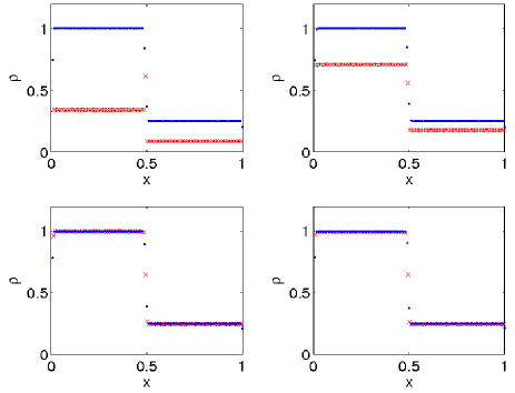
Figure 1: Determination of the Initial density adopting four different SPH algorithms. Left to right, top to bottom: standard SPH, mass density summation; Lagrangian SPH, mass density summation; standard SPH, number density summation; Lagrangian SPH, number density determination. Blue dots: high mass particles; red crosses: low mass particles.

3.1 On symmetrisation

To ensure the conservation of energy and momenta, a proper symmetrisation of the equations of motion is required. It is worth noticing that while in the first formulations of SPH such symmetrisation had to be imposed “ad hoc”, in the Lagrangian derivation it is naturally built-in without any further assumption.

Anyway, the symmetrisation is strictly necessary only when pairwise forces act on couples of particles. Thus, it is not needed when obtaining the density from Eq. 41 and 34, or when the internal energy of a particle is evolved according to Eq. 3. Indeed, symmetrisation of the energy equation may lead to unphysical negative temperatures. For example when cold particles are pushed by a strong source of pressure: in this case, the mechanical expansion leads to a loss of internal energy which, if equally subdivided between the cold and hot phase, may exceed the small energy budget of cold bodies (see e.g. Springel & Hernquist 2002).

Since symmetrisation is not needed in the density summation algorithm, the smoothing length of neighbouring particles is not required to compute the density of a particle $i$. This allows an exact calculation simply gathering position and masses of neighbours, which are known at the beginning of the time-step. On the other hand, after the density loop each particle has its new smoothing length $h$ and it is now possible to use these values in the acceleration calculations, where symmetrisation is needed. Anyway, while in the previous case only particles within $2h_{i}$ were considered neighbours of the particle $i$, in this latter case the symmetrisation scheme requires a particle $j$ to be considered neighbour of particle $i$ if $r_{ij}<2\times\max(h_{i},h_{j})$ .

Note that with this scheme two routines of neighbour searching are necessary: the first one in the density summation, and the second in the force calculation. In practice, when the evaluation of density is being performed, a gather view of SPH is adopted (see Hernquist & Katz 1989); thus, each particle $i$ searches its neighbours using only its own smoothing length $h_{i}$, until the convergence process is completed. In this way, if a particle finds too high or too low a number of neighbours (and therefore must change its smoothing length to repeat the search) it is not necessary to inform the other particles (including those belonging to other processors) about the change that is being made. This would in principle be necessary if a standard gather/scatter mode is adopted. Thus, each particle evaluates its density independently, adjusting its smoothing length on its own, and no further communication among processors is necessary, after the initial gathering of particles positions. Moreover, the search is initially performed using an effective searching radius which is slightly larger than the correct value $2h_{i}$. In this way, the neighbour list will include slightly more particles than effectively needed. However, if at the end of the loop, the smoothing length has to be increased by a small factor, it is not be necessary to repeat the tree-walk to reconstruct the neighbour list. Of course, if the adaptive softening length scheme is adopted the tree-walk will be performed to upgrade $h$ and $\rho$ for SPH particles only, and $\epsilon$ and $\rho_{tot}$ for all particles.

Then, when forces (hydrodynamical forces and, if the adaptive softening length scheme is adopted, gravitational forces too) are evaluated, a new search for neighbours must be made, in which a particle is considered neighbour to another one if the distance between the two is lower than the maximum between the two searching radii. During this second tree-walk, the gravitational force is evaluated together with the construction of the particle’s neighbour list. Finally, correcting terms are computed for hydrodynamics equations of motion ($\nabla h$ terms) and, if necessary, for gravitational interactions (if softening lengths are adaptive), summing the neighbouring particles’ contributions.

3.2 Smoothing and softening lengths for SPH particles

SPH particles under self-gravity have two parameters characterizing their physical properties: the softening length $\epsilon$, which tunes their gravitational interactions with nearby particles, and the smoothing length $h$, used to smooth their hydrodynamical features.

In principle there is no need for these two quantities to be related to one another, because they refer to two distinct actions, and have somehow opposite functions as noted above. However, Bate & Burkert (1997) claimed that a quasi-stable clump of gas could became un-physically stable against collapse if $\epsilon>h$, because in this case pressure forces would dominate over the strongly softened gravity, or on the other hand, if $\epsilon<h$, collapse on scales smaller than the formal resolution of SPH may be induced, causing artificial fragmentation. They recommend that gravitational and hydrodynamical forces should be resolved at the same scale length, imposing $\epsilon=h$ (requiring both of them to fixed, or $\epsilon$ to be adaptive like $h$, with the introduction of the correcting terms described above). In other studies (e.g. Thacker & Couchman 2000) the softening length is fixed, but the smoothing length is allowed to vary imposing a lower limit close to the value of the softening length (this is a typical assumption in SPH simulations of galaxy formation).

Anyway, Williams et al. (2004) have studied the effects of such procedure, finding that in many hydrodynamical studies this can cause a number of problems. The adoption of large values of $h$ can result in over-smoothed density fields, i.e. a decrease in the computed values of density $\rho$ and of density gradients $\nabla\rho$, which in turn un-physically decreases the computed pressure accelerations in the Euler equation. Problems with angular momentum transfer may also arise. Therefore, they suggest to allow $h$ to freely vary. This eventually yields improved accuracy and also, contrary to expectations, a significant saving in computational time (because the number of neighbours is kept fixed instead of largely increasing as it may happen in dense environments with fixed $h$). Moreover, they pointed out that, in contrast with the claims by Bate & Burkert (1997), the smoothing length should not be kept equal to the softening length, because in many physical situations (shocks for example) hydrodynamical forces dominate over gravity and likely need to be properly resolved on size scales smaller than the softening length.

Finally, a numerical problem arises when trying to keep $\epsilon=h$ in cosmological simulations. The presence of a Dark Matter component makes it impossible to keep constant the number of both hydrodynamical and gravitational neighbours. For example, a collapsed Dark Matter halo could retain few gaseous particles (because of shocks and/or stellar feedback), and these will thus have many gravitational neighbours but few hydrodynamic neighbours with a unique softening/smoothing length. The opposite problem could arise in the case of very dense clumps of cold gas that may form behind shocks, without a corresponding concentration of Dark Matter.

Thus, in EvoL both $\epsilon$ and $h$ are let free to vary independently from one another. Future tests may be done trying to keep the two parameters linked, for example allowing for some variations in both their ratio $\epsilon/h$ (imposing it to be around, but not exactly, 1) and in the number of hydrodynamical and gravitational neighbours.

3.3 Discontinuities

3.3.1 Artificial viscosity

The SPH formalism in its straight form is not able to handle discontinuities. By construction, SPH smooths out local properties on a spatial scale of the order of the smoothing length $h$. Anyway, strong shocks are of primary importance in a number of astrophysical systems. Thus, to model a real discontinuity in the density and/or pressure field ad hoc dissipational, pressure-like terms must be added to the perfect fluid equations, to spread the discontinuities over the numerically resolvable length. This is usually achieved by introducing an artificial viscosity, a numerical artifact that is not meant to mimic physical viscosity, but to reproduce on large scale the action of smaller, unresolved scale physics, with a formulation consistent with the Navier-Stockes terms.

Among the many formulations that have been proposed, the most commonly used is obtained adding a term $\Pi_{ij}$ to the Eqs. 3 and 3, so that

$$\frac{d\@vec{v}_{i}}{dt} = \sum_{j}m_{j}\times$$

$$\left[\frac{P_{i}}{\rho_{i}^{2}}\left(1+\frac{\zeta_{i}/m_{j}}{\Omega_{i}^{*}}\right)\nabla_{i}W_{ij}(h_{i})+\right.$$

$$\left.\frac{P_{j}}{\rho_{j}^{2}}\left(1+\frac{\zeta_{j}/m_{i}}{\Omega_{j}^{*}}\right)\nabla_{i}W_{ij}(h_{j})+\Pi_{ij}\bar{\nabla_{i}W_{ij}}\right],$$

and

$$\frac{du_{i}}{dt} =$$

$$\sum_{j}m_{j}\left[\frac{P_{i}}{\rho_{i}^{2}}\left(1+\frac{\zeta_{i}/m_{j}}{\Omega_{i}^{*}}\right)(\@vec{v}_{j}-\@vec{v}_{i})\cdot\nabla_{i}W_{ij}(h_{i})\right.$$

$$+\left.\frac{1}{2}\Pi_{ij}w_{ij}|\bar{\nabla_{i}W_{ij}}|\right].$$

Here $w_{ij}=(\@vec{v}_{ij}\cdot\@vec{r}_{ij})/|\@vec{r}_{ij}|$,

$$\Pi_{ij}=\begin{cases}\left(\frac{-\alpha\bar{c_{ij}}\mu_{ij}+\beta\mu_{ij}^{2}}{\bar{\rho_{ij}}}\right)&\text{if $\@vec{v}_{ij}\cdot\@vec{r}_{ij}<0$,}\\ 0&\text{if $\@vec{v}_{ij}\cdot\@vec{r}_{ij}\geq 0$,}\end{cases}$$ (57)

$$\mu_{ij}=\frac{h\@vec{v}_{ij}\cdot\@vec{r}_{ij}}{\@vec{r_{ij}^{2}}+\eta^{2}},$$ (58)

and

$$\bar{\nabla_{i}W_{ij}} =$$

$$\frac{1}{2}\left[\nabla_{i}W_{ij}(h_{i})\left(1+\frac{\zeta_{i}/m_{j}}{\Omega_{i}^{*}}\right)\right.$$

$$\left.+\nabla_{i}W_{ij}(h_{j})\left(1+\frac{\zeta_{j}/m_{i}}{\Omega_{j}^{*}}\right)\right]$$

(Monaghan 1988). $\bar{c_{ij}}$ is the average sound speed, which is computed for each particle from a suitable equation of state (EoS), like the ideal monatomic gas EoS $P=(\gamma-1)\rho u$, using $c_{i}=\sqrt{\gamma(\gamma-1)u_{i}}$ ($\gamma$ is the adiabatic index); the parameter $\eta$ is introduced to avoid numerical divergences, and it is usually taken to be $\eta=0.1h$. $\alpha$ and $\beta$ are two free parameters, of order unity, which account respectively for the shear and bulk viscosity in the Navier-Stokes equation (Watkins et al. 1996), and for the von Neuman-Richtmyer viscosity, which works in high Mach number flows.

A more recent formulation is the so-called “signal velocity” viscosity (Monaghan 1997), which works better for small pair separations between particles, being a first-order expression of $h/r$; it reads

$$\Pi_{ij}=\frac{-\alpha v_{ij}^{sig}w_{ij}}{\bar{\rho_{ij}}},$$ (61)

with the signal velocity defined as

$$v_{ij}^{sig}=2\bar{c_{ij}}-w_{ij}.$$ (62)

One or the other of the two formulations above can be used in EvoL.

In general, artificial dissipation should be applied only where really necessary. However, it has long been recognized that artificial viscosity un-physically boosts post-shock shear viscosity, suppressing structures in the velocity field on scales well above the nominal resolution limit, and damping the generation of turbulence by fluid instabilities.

To avoid the overestimate of the shear viscosity, Balsara (1995) proposed to multiply the chosen expression of $\Pi_{ij}$ by a function $\bar{f_{ij}}=(f_{i}+f_{j})/2$; the proposed expression for the “limiter” $f_{i}$ for a particle $i$ is

$$f_{i}=\frac{|\nabla_{i}\cdot\@vec{v}_{i}|}{|\nabla_{i}\cdot\@vec{v}_{i}|+|\nabla_{i}\times\@vec{v}_{i}|+\eta c_{i}/h_{i}},$$ (63)

where $\eta\sim 10^{-4}$ is a factor introduced to avoid numerical divergences. It can be seen that $f$ acts as a limiter reducing the efficiency of viscous forces in presence of rotational flows.

Another possible cure to the problem is as follows. The most commonly used values for the parameters $\alpha$ and $\beta$ in Eq. 57 are $\alpha=1$ and $\beta=2$. Bulk viscosity is primary produced by $\alpha$, and this sometimes over-smoothen the post-shock turbulence. To cope with this, Morris & Monaghan (1997) have proposed a modification to Eq. 57, in which the parameter $\alpha$ depends on the particle and changes with time according to:

$$\frac{d\alpha_{i}}{dt}=-\frac{\alpha_{i}-\alpha_{min}}{\tau}+G_{i},$$ (64)

where $\alpha_{min}=0.01$ is the minimum allowed value, $\tau=0.1h_{i}/v^{sig}$ is an $e$-folding time scale (with $v^{sig}=\max_{j}[v_{ij}^{sig}]$), and $G_{i}$ is a source term which can be parameterized as $G_{i}=0.75f_{i}\max[0,-|\nabla\cdot\@vec{v}_{i}|]$. This formulation embodies some different prescriptions (e.g. in Rosswog & Price 2007; Price 2008). In Eq. 61, one can then put $\alpha=\frac{1}{2}(\alpha_{i}+\alpha_{j})$. Dolag et al. (2005) have shown that this scheme captures shocks as well as the original formulation of SPH, but, in regions away from shocks, the numerical viscosity is much smaller. In their high resolution cluster simulations, this resulted in higher levels of turbulent gas motions in the ICM, significantly affecting radial gas profiles and bulk cluster properties. Interestingly, this tends to reduce the differences between SPH and adaptive mesh refinement simulations of cluster formation.

3.3.2 Artificial thermal conductivity

As Price (2008) pointed out, an approach similar to that described above should be used to smooth out discontinuities in all physical variables. In particular, an artificial thermal conductivity is necessary to resolve discontinuities in thermal energy (even if only a few formulations of SPH in literature take this into account).

The artificial thermal conductivity is represented by the term

$$\Pi^{u}=-\frac{\bar{\alpha_{ij}^{u}}v_{sig}^{u}(u_{i}-u_{j})}{\bar{\rho_{ij}}}.$$ (65)

Here $\alpha^{u}$ is a conductivity coefficient, $\frac{1}{2}(\alpha_{i}^{u}+\alpha_{j}^{u})$ that varies with time according to

$$\frac{d\alpha_{i}^{u}}{dt}=-\frac{\alpha_{i}^{u}-\alpha^{u}_{min}}{\tau}+S_{i}^{u},$$ (66)

where $\tau$ is the same time scale as above, $\alpha^{u}_{min}$ is usually $0$, and the source term can be defined as $S_{i}^{u}=h_{i}|\nabla^{2}u_{i}|/\sqrt{u_{i}}$ (Price 2008), in which the expression for the second derivative is taken from Brookshaw (1986)

$$\nabla^{2}u_{i}=\sum_{j}2m_{j}\frac{u_{i}-u_{j}}{\rho_{j}}\frac{|\bar{\nabla_{i}W_{ij}}|}{r_{ij}}$$ (67)

which reduces particles noise; $v_{ij}^{sig}$ can be either the same quantity defined in Eq. 62 or

$$v_{ij}^{sig}=\sqrt{\frac{|P_{i}-P_{j}|}{\rho_{ij}}}$$ (68)

In passing, we note that adopting the source term suggested by Price & Monaghan (2005), $S_{i}^{u}=0.1h_{i}|\nabla^{2}u_{i}|$, would be less accurate in problems requiring an efficient thermal conduction such as the standard shock tube test with un-smoothed initial conditions, see Sect. 5.

The term $\Pi^{u}$ must finally be added to Eq. 3.3.1, giving

$$\frac{du_{i}}{dt} =$$

$$\sum_{j}m_{j}\left[\frac{P_{i}}{\rho_{i}^{2}}\left(1+\frac{\zeta_{i}/m_{j}}{\Omega_{i}^{*}}\right)(\@vec{v}_{j}-\@vec{v}_{i})\cdot\nabla_{i}W_{ij}(h_{i})\right.$$

$$+\left.\left(\frac{1}{2}\Pi_{ij}+\Pi_{ij}^{u}\right)w_{ij}|\bar{\nabla_{i}W_{ij}}|\right].$$

As in the case of artificial viscosity, it is worth noting that this conductive term is not intended to reproduce a physical dissipation; instead, it is a merely numerical artifact introduced to smooth out unresolvable discontinuities.

3.4 Entropy equation

Instead of looking at the thermal energy, we may follow the evolution of a function of the total particle entropy, for instance the entropic function

$$A(s)=\frac{P}{\rho^{\gamma}},$$ (70)

where $\gamma$ is the adiabatic index. This function is expected to grow monotonically in presence of shocks, to change because of radiative losses or external heating, and to remain constant for an adiabatic evolution of the gas. Springel & Hernquist (2002) suggest the following SPH expression for the equation of entropy conservation:

$$\frac{dA_{i}}{dt} = -\frac{\gamma-1}{\rho_{i}^{\gamma}}S(\rho_{i},u_{i})$$

$$+\frac{1}{2}\frac{\gamma-1}{\rho_{i}^{\gamma-1}}\sum_{j}m_{j}\Pi_{ij}\@vec{v}_{ij}\cdot\nabla_{i}W_{ij},$$

where $S$ is the source function describing the energy losses or gains due to non adiabatic physics apart from viscosity. If $S<<1$, the function $A(s)$ can only grow in time, because of the shock viscosity. Eq. 3.4 can be integrated instead of Eq. 3.3.1 giving a more stable behaviour in some particular cases. Note that internal energy and entropic function of a particle can be related via

$$u=\frac{A(s)}{\gamma-1}\rho^{\gamma-1}.$$ (72)

The entropic function can be used to detect situations of shocks, since its value only depends on the strength of the viscous dissipation.

In general, if the energy equation is used (integrated), the entropy is not exactly conserved, and viceversa. Moreover, if the density is evolved according to the continuity Eq. 38 and the thermal energy according to Eq. 3, both energy and entropy are conserved; but in this case the mass is not be conserved (to ensure this latter, density must be computed with Eq. 34). This problem should be cured with the inclusion of the $\nabla h$ terms in the SPH method, as already discussed.

3.5 X-SPH

As an optional alternative, EvoL may adopt the smoothing of the velocity field by replacing the normal equation of motion $d\@vec{r}_{i}/dt=\@vec{v}_{i}$ with

$$\frac{d\@vec{r}_{i}}{dt}=\@vec{v}_{i}+\eta\sum_{j}m_{j}\left(\frac{\@vec{v_{ji}}}{\bar{\rho_{ji}}}\right)W_{ij},$$ (73)

(Monaghan 1992) with $\bar{\rho_{ji}}=(\rho_{i}+\rho_{j})/2$, $\@vec{v_{ji}}=\@vec{v}_{j}-\@vec{v}_{i}$, and $\eta$ constant, $0\leq\eta\leq 1$. In this variant of the SPH method, known as X-SPH, a particle moves with a velocity closer to the average velocity in the surroundings. This formulation can be useful in simulations of weakly incompressible fluids, where it keeps particles in order even in absence of viscosity, or to avoid undesired inter-particle penetration.

4 Description of the Code: Integration

4.1 Leapfrog integrator

Particles positions and velocities are advanced in time by means of a standard leapfrog integrator, in the so-called Kick-Drift-Kick (KDK) version, where the K operator evolves velocities and the D operator evolves positions:

$$\mbox{{K${}_{1/2}$}: }\@vec{v_{n+1/2}}=\@vec{v_{n}}+\frac{1}{2}\@vec{a(\@vec{r_{n}})}\delta t$$

$$\mbox{{D: }}\@vec{r_{n+1}}=\@vec{r_{n}}+\@vec{v_{n+1/2}}\delta t$$

$$\mbox{{K${}_{1/2}$}: }\@vec{v_{n+1}}=\@vec{v_{n+1/2}}+\frac{1}{2}\@vec{a(\@vec{r_{n+1}})}\delta t.$$

A predicted value of physical quantities at the end of each time-step is also predicted at the beginning the same step, to guarantee synchronization in the calculation of the accelerations and other quantities. In particular, in the computation of the viscous acceleration on gas particles the synchronized predicted velocity $\@vec{v_{n+1}}=\@vec{v_{n}}+\@vec{a(\@vec{r_{n}})}\delta t$ is used.

Moreover, if the individual time-stepping is adopted (see below, Sect. 4.2.1), non-active particles use predicted quantities to give their own contributions to forces and interactions.

4.2 Time-stepping

A trade-off between accuracy and efficiency can be reached by a suitable choice of the time-step. One would like to obtain realistic results in a reasonable amount of CPU time. To do so, numerical stability must be ensured, together with a proper description of all relevant physical phenomena, at the same time reducing the computational cost keeping the time-step as large as possible.

To this aim, at the end of each step, for each particle the optimal time-step is given by the shortest among the following times:

$$\delta t_{acc,i}=\eta_{acc}\sqrt{\frac{min(\epsilon_{i},h_{i})}{|\@vec{a}_{i}|}}$$

$$\delta t_{vel,i}=\eta_{vel}\sqrt{\frac{min(\epsilon_{i},h_{i})}{|\@vec{v}_{i}|}}$$

$$\delta t_{av,i}=\eta_{av}\sqrt{\frac{|\@vec{v}_{i}|}{|\@vec{a}_{i}|}}$$

with obvious meaning of symbols; the parameters $\eta$’s are of the order of $0.1$. The third of these ratios, under particular situations, can assume extremely small values, and should therefore be used with caution.

We can compute two more values, the first obtained from the well known Courant condition and the other constructed to avoid large jumps in thermal energy:

$$\delta t_{C,i}=\eta_{C}\frac{h_{i}}{h_{i}|\nabla\cdot\@vec{v}_{i}|+c_{i}+1.2(\alpha c_{i}+\beta\max_{j}|\mu_{ij}|)}$$

$$\delta t_{u,i}=\eta_{u}\left|\frac{u_{i}}{du_{i}/dt}\right|$$

where $\alpha,\beta$ and $\mu$ are the quantities defined in the artificial viscosity parametrization, see Sect. 3.3.1, and $c$ is the sound speed.

If the simulation is run with a global time-stepping scheme, all particles are advanced adopting the minimum of all individual time-steps calculated in this way; synchronization is clearly guaranteed by definition.

If desired, a minimum time-step can be imposed. In this case, however, limiters must be adopted to avoid numerical divergences in accelerations and/or internal energies. This of course leads to a poorer description of the physical evolution of the system; anyway, in some cases a threshold may be necessary to avoid very short time-steps due to violent high energy phenomena.

4.2.1 Individual time-stepping

Cosmological systems usually display a wide range of densities and temperatures, so that an accurate description of very different physical states is necessary within the same simulation. Adopting the global time-stepping scheme may cause a huge waste of computational time, since gas particles in low-density environments and collisionless particles generally require much longer time-steps than the typical high-density gas particle.

In EvoL an individual time-stepping algorithm can be adopted, which makes a better use of the computational resources. It is based on a powers-of-two scheme, as in Hernquist & Katz (1989). All individual particles real time steps, $\delta t_{i,true}$, are chosen to be a power-of-two subdivision of the largest allowed time-step (which is fixed at the beginning of the simulation), i.e.

$$\delta t_{i,true}=\delta t_{max}/2^{n_{i}},$$ (74)

where $n_{i}$ is chosen as the minimum integer for which the condition $\delta t_{i,true}\geq\delta t_{i}$ is satisfied. Particles can move to a smaller time bin (i.e. a longer time step) at the end of their own time step, but are allowed to do so only if that time bin is currently time-synchronized with their own time bin, thus ensuring synchronization at the end of every largest time step.

A particle is then marked as “active” if $t_{i}+\delta t_{i,true}=t_{sys}$, where the latter is the global system time, updated as $t_{sys,new}=t_{sys,old}+\delta t_{sys}$, where $\delta t_{sys}=min(\delta t_{i})$. At each time-step, only active particles re-compute their density and update their accelerations (and velocities) via summation over the tree and neighboring particles. Non-active particles keep their acceleration and velocity fixed and only update their position using a prediction scheme at the beginning of the step. Note that some other evolutionary features (i.e. cooling or chemical evolution) are instead updated at every time-step for all particles.

Since in presence of a sudden release of very hot material (e.g. during a Supernova explosion) one or a few particles may have to drastically and abruptly reduce their time-step, the adoption of individual time-stepping scheme would clearly lead to unphysical results, since neighbouring non-active particles would not notice any change until they become active again. This is indeed a key issue, very poorly investigated up to now. To cope with this, a special recipe has been added, forcing non-active particles to “wake up” if they are being shocked by a neighbour active particle, or in general if their time-step is too long (say more than 4-8 times bigger) with respect to the minimum time-step among their neighbours. In this way, when an active particle suddenly changes its physical state, all of its neighbouring particles are soon informed of the change and are able to react properly. Saitoh & Makino (2008) recently studied the problem, coming to similar conclusions and recommending a similar prescription when modelling systems in which sudden releases of energy are expected.

Note that when a non-active particle is waken up energy and momentum are not perfectly conserved, since its evolution during the current time-step is not completed. Anyway, this error is negligible if compared to the errors introduced by ignoring this correction.

4.3 Periodic boundary conditions

Periodic boundary conditions are implemented in EvoL using the well known Ewald (1921) method, i.e. adding to the acceleration of each particle an extra-term due to the replicas of particles and nodes, expanding in Fourier series the potential and the density fluctuation, as described in Hernquist et al. (1991) and in Springel et al. (2001). If $\@vec{x}_{i}$ is the coordinate at the point of force-evaluation relative to a particle or a node $j$ of mass $m_{j}$, the additional acceleration that must be added to account for the action of the infinite replicas of $j$ is given by

$$acc_{per}(\@vec{x})=m_{j}\left[\frac{\@vec{x}}{|\@vec{x}|^{3}}-\sum_{n}\frac{\@vec{x}-\@vec{n}L}{|\@vec{x}-\@vec{n}L|^{3}}\times\right.$$ (75)

$$\left(erfc(\omega|\@vec{x}-\@vec{n}L|)+\frac{2\omega|\@vec{x}-\@vec{n}L|}{\sqrt{\pi}}\times e^{-\omega^{2}|\@vec{x}-\@vec{n}L|^{2}}\right)$$

$$\left.-\frac{2}{L^{2}}\sum_{\@vec{h}/=0}\frac{\@vec{h}}{|\@vec{h}|^{2}}e^{-\frac{\pi^{2}|\@vec{h}|^{2}}{\omega^{2}L^{2}}}sin\left(\frac{2\pi}{L}\@vec{h}\cdot\@vec{x}\right)\right]$$

where $\@vec{n}$ and $\@vec{h}$ are integer triplets, $L$ is the periodic box size, and $\omega$ is an arbitrary number. Convergence is achieved for $\omega=2/L$, $|\@vec{n}|<5$ and $|\@vec{h}|<5$ (Springel et al. 2001). The correcting terms $acc_{per}/m_{j}$ are tabulated, and trilinear interpolation off the grid is used to compute the correct accelerations. It must be pointed out that this interpolation significantly slows down the tree algorithm, almost doubling the CPU time.

Periodism in the SPH scheme is obtained straightforwardly finding neighbours across the spatial domain and taking the modulus of their distance, in order to obtain their nearest image with respect to the active particle. In this way, no ghost particles need to be introduced.

4.4 Parallelization

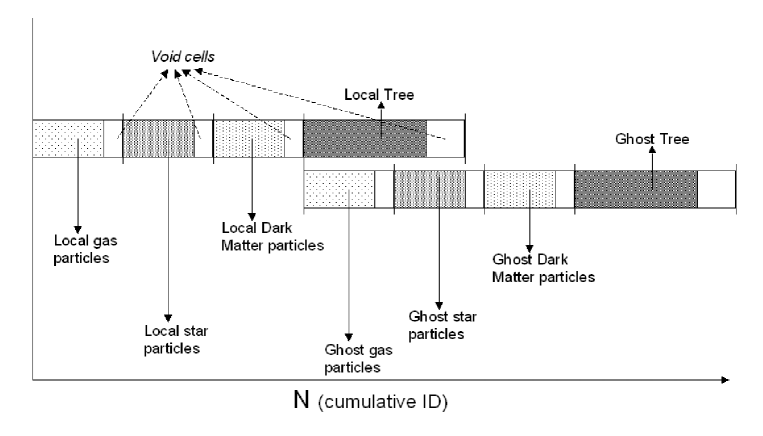
Figure 2: Data structures in EvoL. Void cells are included to allow for new particles to be created and/or imported from other CPUs. Ghost structures are reallocated at each time-step.

EvoL uses the MPI communication protocol to run in parallel on multiple CPUs. First of all, particles must be subdivided among the CPUs, so that each processor has to deal only with a limited subset of the total number of bodies. To this aim, at each time-step the spatial domain is subdivided using the Orthogonal Recursive Bisection (ORB) scheme. In practice, each particle keeps track of the time spent to compute its properties during the previous time-step in which it has been active, storing it in a work-load variable. At the next time-step the spatial domain is subdivided trying to assign to each CPU the same total amount of work-load (only considering active particles if the individual time-stepping option is selected), re-assigning bodies near the borders among the CPUs. To this aim, the domain is first cut along the $x$-axis, at the coordinate $x_{cut}$ that better satisfies the equal work-load condition among the two groups of CPUs formed by those with geometrical centers $x_{centre}\leq x_{cut}$ and those with $x_{centre}>x_{cut}$. In practice, each CPU exchanges particles only if its borders are across $x_{cut}$. Then, the two groups of CPUs are themselves subdivided into two new groups, this time cutting along the $y$-axis (at two different coordinates, because they are independent from one another having already exchanged particles along the $x$-axis). The process is iterated as long as required (depending to the number of available CPUS) cutting recursively along the three dimensions. It should be noted that this scheme allows to use only a power-of-two number of CPUs, whereas other procedures (e.g. a Peano-Hilbert domain decomposition, see e.g. Springel 2005) can more efficient exploit the available resources.

It may sometimes happen that a CPU wants to acquire more particles than permitted by the dimensions of its arrays. In this case, data structures are re-allocated using temporary arrays to store extra-data, as described in the next Section.

Apart from the allocation of particles to the CPUs, the other task for the parallel architecture is to spread the information about particles belonging to different processors. This is achieved by means of “ghost” structures, in which such properties are stored when necessary. A first harvest among CPUs is made at each time step before computing SPH densities: at this point, positions, masses and other useful physical features of nearby nodes and particles, belonging to other processors, are needed. Each CPU “talks” only to another CPU per time, first importing all the data-structures belonging to it in temporary arrays, and then saving within its “ghost-tree” structure only the data relative to those nodes and particles which will be actually used. For example, if a “ghost node” is sufficiently far away from the active CPU geometrical position so that the gravitational opening criterion is satisfied, there will be no need to open it to compute gravitational forces, and no other data relative to the particles and sub-nodes it contains will be stored in the ghost-tree.

A second communication among CPUs is necessary before computing accelerations. Here, each particle needs to known the exact value of the smoothing and softening lengths (which have been updated during the density evaluation stage) as well as many other physical values of neighbouring (but belonging to different CPUs) particles. The communication scheme is exactly the same as before, involving ghost structures. It was found that, instead of upgrading the ghost-tree built before the density evaluation, a much faster approach is to completely re-build it.

The dimensions of the ghost arrays are estimated at the beginning of the simulation, and every $N$ time-steps (usually, $N=100$), by means of a “preliminary walk” among all CPUs. In intermediate steps, the dimensions of these arrays are modified on the basis of the previous step evaluation and construction of ghost structures.

4.5 Data structures

All data structures are dynamically adapted to the size of the problem under exploration. In practice, at the beginning of a simulation, all arrays are allocated so that their dimension is equal to the number of particles per processor, plus some empty margin to allow for an increase of the number of particles to be handled by the processor (see Fig. 2).

Anyway, whenever a set of arrays within a processor becomes full of data and has no more room for new particles, the whole data structure of that processor is re-scaled increasing its dimensions, to allow for new particles to be included. Of course, also the opposite case (i.e. if the number of particles decreases, leaving too many void places) is considered.

To this aim, the data in excess are first stored in temporary T arrays. Then, the whole “old” data structure O is copied onto new temporary N arrays, of the new required dimensions. Finally, T arrays are copied into the N structure; this substitutes the O structure, which is then deleted. Clearly, this procedure is quite memory-consuming. Anyway, it ideally has to be carried out only a few times per simulation, at least in standard cases. Moreover, it is performed after the “ghost” scheme described above has been completed, and ghost-structures have been deallocated, leaving room for other memory-expensive routines.

5 Tests of the code

An extended set of hydrodynamical tests have been performed to check the performance of EvoL under different demanding conditions:

• Rarefaction and expansion problem (Einfeldt et al. 1991, 1D);

• Shock tube problem (Sod 1978, both in 1D and in 3D);

• Interacting blast waves (Woodward & Colella 1984, 1D);

• Strong shock collapse (Noh 1987, 2D);

• Kelvin-Helmholtz instability problem (2D);

• Gresho vorticity problem (Gresho & Chan 1990, 2D);

• Point-like explosion and blast wave (Sedov-Taylor problem, 3D);

• Adiabatic collapse (Evrard 1988, 3D);

• Isothermal collapse (Boss & Bodenheimer 1979, 3D);

• Collision of two politropic spheres (3D);

• Evolution of a two-component fluid (3D).

Except where explicitly pointed out, the tests have been run on a single CPU, with the global time-stepping algorithm, and adopting the following parameters for the SPH scheme: $\eta=1.2$, $\alpha_{max}=2$, $\alpha_{min}=0.01$, $\beta=2\alpha$, $\gamma=5/3$, and equation of state $P=(\gamma-1)\rho u$. Where gravitation is present, the opening angle for the tree code has been set $\theta=0.8$. The tests in one and two dimensions have been run adopting the kernel formulations shown in Appendix A. The exact analytical solutions have been obtained using the software facilities freely available at the website http://cococubed.asu.edu/code_pages/codes.shtml.

5.1 Rarefaction wave

We begin our analysis with a test designed to check the the code in extreme, potentially dangerous low-density regions, where some iterative Riemann solvers can return negative values for pressure/density. In the Einfeldt rarefaction test (Einfeldt et al. 1991) the two halves of the computational domain $0<x<1$ move in opposite directions, and thereby create a region of very low density near the initial velocity discontinuity at $x=0.5$. The initial conditions of this test are

$$\begin{cases}\rho=1.0,\mbox{ }P=0.4,\mbox{ }v_{x}=-2.0,&\text{for $x<0.5$,}\\ \rho=1.0,\mbox{ }P=0.4,\mbox{ }v=2.0,&\text{for $x\geq 0.5$.}\end{cases}$$ (76)

The results at $t=0.2$ for a 1-D, 1000-particle calculation are shown in Fig. 3. Clearly, the low-density region is well described by the code.

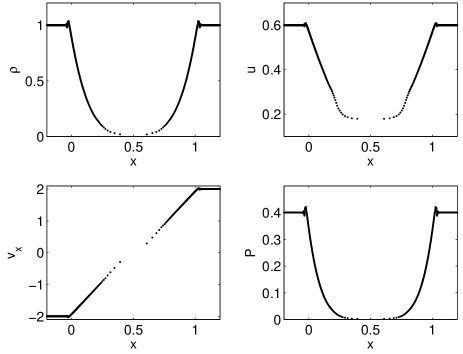
Figure 3: Left to right, top to bottom: density, internal energy, x-velocity, and pressure profiles at t=0.2 for the Einfeldt test. All quantities are in code units.

5.2 Shock Tube

The classic Riemann problem to check the shock capturing capability is the Sod’s shock tube test (Sod 1978). We run many different cases changing numerical parameters, to check the response to different settings. All tests have been started from un-smoothed initial conditions, leaving the code to smear out the initial discontinuities.

5.2.1 1-D tests

The first group of tests have been performed in one dimension. 1,000 equal mass particles have been displaced on the $x$ axis, in the domain $0\leq x\leq 1$, and changing inter-particle spacing, to obtain the following setting:

$$\begin{cases}\rho=1.0,\mbox{ }u=1.5,\mbox{ }v=0,&\text{for $x<0.5$,}\\ \rho=0.25,\mbox{ }u=1.077,\mbox{ }v=0,&\text{for $x\geq 0.5$.}\end{cases}$$ (77)

($m=6.25\times 10^{-4}$). In this way, particles belonging to the left region of the tube initially have $P=1$, whereas particles on the right side of the discontinuity have $P=0.1795$, as in the classic Monaghan & Gingold (1983) test. We performed four runs:

• T1 - standard viscosity (with $\alpha=1$ and $\beta=2$) and no artificial conduction;

• T2 - standard viscosity plus artificial conduction;

• T3 - viscosity with variable $\alpha$ plus artificial conduction;

• T4 - the same as T2, but with the same density discontinuity obtained by using particles with different masses on a regular lattice instead of equal mass particles shrinking their spacing. To do so, particles in the left part of the tube have the mass $m=10^{-3}$, whereas those in the right part have $m=2.5\times 10^{-4}$.

Figure 4: Left to right, top to bottom: density, internal energy, x-velocity and pressure profiles at t=0.12 for test T1 see text for details. Red solid line: exact solution. Alla quantities are in code units.

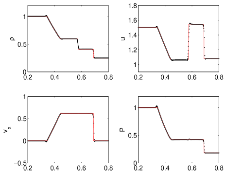
Figure 5: the same as in Fig. 4, but for the test T2 (see text for details).

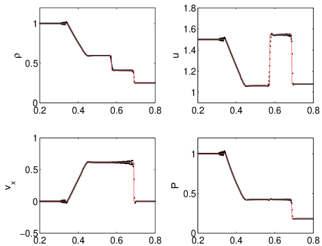
Figure 6: The same as in Fig. 4, but for the test T3 (see text for details).

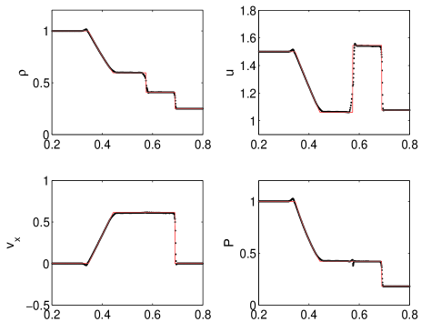
Figure 7: The same as in Fig. 4, but for the test T4 (see text for details).

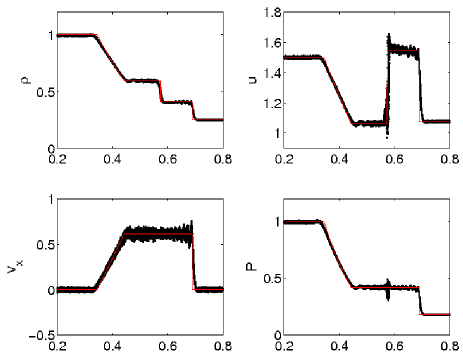
Figure 8: The same as in Fig. 4, but for the test T5 (see text for details).

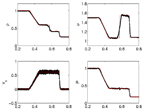
Figure 9: The same as in Fig. 4, but for the test T6 (see text for details).

Figs. 4 through 7 show the density, internal energy, $x$-velocity and pressure $x$-profiles at $t=0.12$ for the four cases (in code units).

The overall behaviour is good in all cases. We note the typical blip in the pressure profile and the wall-like overshoot in thermal energy at the contact discontinuity in the T1 run. The introduction of the artificial thermal conductivity (T2) clearly cures the problem at the expense of a slightly shallower thermal energy profile. Introducing the variable $\alpha$-viscosity (T3), the reduced viscosity causes post-shock oscillations in the density (and energy), and makes the velocity field noisier and turbulent, as expected.

Little differences can be seen in the T4 run, except for a slightly smoother density determination at the central contact discontinuity, which also makes the blip problem worse. Thus, the best results are obtained with the T2 configuration.

5.2.2 3-D tests

As pointed out by Steinmetz & Mueller (1993), performing shock tube calculations with 1-D codes, with particles initially displaced on a regular grid, makes the effects of numerical diffusivity essentially negligible, but in realistic cosmological 3-D simulations the situation is clearly more intrigued. To investigate this issue, we switch to a 3-D description of the shock tube problem. The initial conditions are set using a relaxed glass distribution of $\sim 60,000$ particles, in a box of dimensions $[0,1]$ along the $x$ axis and (periodic) $[0,0.1]$ along the $y$ and $z$ axis. Particles are assigned a mass $m_{right}=1.71\times 10^{-7}$ and $m_{left}=2.5\times m_{right}$ on the two sides on the discontinuity at $x=0.5$, with all other parameters as in the 1-D case. A first run (T5) was performed adopting the T1 configuration (standard viscosity, no artificial conduction), while a second one (T6) was performed switching on the artificial conduction term.

Figs. 8 and 9 show the state of the system at $t=0.12$ in the two cases (note that all particles and not mean values are plotted). As in the 1-D case, the overall agreement with the theoretical expectation is quite good. However, the inclusion of the conductive term on one hand yields sharper profiles and reduces the pressure blip, on the other hand gives a smoother description of contact discontinuities (see the density profile at $x=0.55$). We argue that part of the worse results may be due to the use of particles with different mass as a similar result has been found with the corresponding 1-D test (see T4 above). A limit on the conduction efficiency could give better results, but and ad hoc adjustment should be applied to each case.

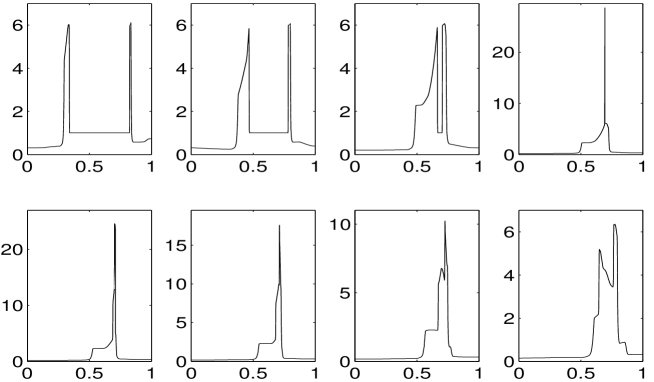
Figure 10: Left to right, top to bottom: density profiles at $t=0.010$, $t=0.016$, $t=0.026$, $t=0.028$, $t=0.030$, $t=0.032$, $t=0.034$, $t=0.038$ for the Woodward high-resolution test (see text for details). All quantities are in code units.

5.3 Interacting blast waves

Woodward & Colella (1984) proposed a severe test in 1-D, i.e. two strong blast waves develop out of a gas of density $\rho=1$ initially at rest in the domain $0<x<1$, with pressure $P=1000$ for $x<0.1$, $P=100$ for $x>0.9$ and $P=0.01$ in between (the adiabatic index is $\gamma=1.4$). The boundary conditions are reflective on both sides; this can be achieved introducing ghost particles created on-the-fly. Evolving in time, the two blast waves give rise to multiple interactions of strong shocks, rarefaction and reflections.

We performed two runs: one at high resolution with 1000 equally spaced particles, and one at low resolution with only 200 particles. In both cases, the code included the artificial conduction, and viscosity with constant $\alpha=1$.

Fig. 10 shows the density $x$-profiles for the high resolution case, at $t=0.010$, 0.016, 0.026, 0.028, 0.030, 0.032, 0.034, 0.038. The results can be compared with those of Woodward & Colella (1984), Steinmetz & Mueller (1993) and Springel (2009). The complex evolution of the shock and rarefaction waves is reproduced with good accuracy and with sharp profiles, in nice agreement with the theoretical expectations. The very narrow density peak at $t=0.028$, which should have $\rho\approx 30$, is well reproduced and only slightly underestimated.

Fig. 11 shows the comparison between the density profiles of the high and low resolution cases, at $t=0.038$. The low-resolution one shows a substantial smoothing of the contact discontinuities; nevertheless, the overall behaviour is still reproduced, shock fronts are located at the correct positions, and the gross features of the density profile are roughly reproduced.

5.4 Kelvin-Helmoltz instability

The Kelvin-Helmoltz (KH) instability problem is a very demanding test. Recently, Price (2008) replied to the claim by Agertz et al. (2007) that the SPH algorithm is not able to correctly model contact discontinuities like the Kelvin-Helmoltz (KH) problem. He showed how the inclusion of the conductive term is sufficient to correctly reproduce the instability. We try to reproduce his results running a similar test, using the 2-D version of EvoL.

We set up a regular lattice of particles in the periodic domain $0<x<1$, $0<y<1$, using $256^{2}$ particles. The initial conditions are similar to those adopted by Price (2008). The masses of particles are assigned in such a way that $\rho=2$ for $|y-0.5|<0.25$, and $\rho=1$ elsewhere (note that in Price 2008,   this density difference was instead obtained changing the disposition of equal mass particles). The regions are brought to pressure equilibrium with $P=2.5$. In this case, although the initial gradients in density and thermal energy are not smoothed, the thermal energy is assigned to the particles after the first density calculation, to ensure a continuous initial pressure field.

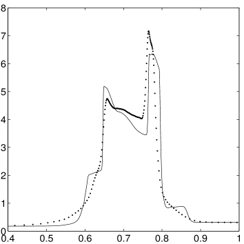
Figure 11: Comparison between high-resolution (solid line) and low-resolution (dots) density profiles at $t=0.038$ for the Woodward test (see text for details). The quantities are in code units.

The initial velocity of the fluid is set as follows:

$$v_{x}=\begin{cases}0.5&\text{if $|y-0.5|<0.25$,}\\ -0.5&\text{if $|y-0.5|\geq 0.25$,}\\ \end{cases}$$ (78)

and

$$v_{y} = w_{0}\sin(4\pi x)\times$$

$$\left\{\exp\left[-\frac{(y-0.25)^{2}}{2\sigma^{2}}\right]+\exp\left[-\frac{(y-0.75)^{2}}{2\sigma^{2}}\right]\right\},$$

where we use $\sigma=0.05/\sqrt{2}$, and $w_{0}=0.1$ or $w_{0}=0.25$ for two different runs (K1 and K2, respectively). In this way, a small perturbation in the velocity field is forced near the contact discontinuity, triggering the instability.

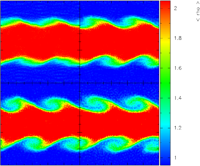
Figure 12: Kelvin-Helmoltz instability according to test K1. Left to right, top to bottom: density field at $t=0.768$, $t=1.158$, $t=1.549$ and $t=1.940$. All quantities are in code units.

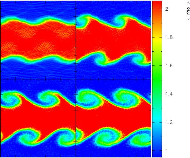
Figure 13: Kelvin-Helmoltz instability according to test K2. Left to right, top to bottom: density field at $t=0.377$, $t=0.767$, $t=1.158$ and $t=1.549$. All quantities are in code units.

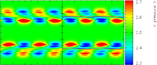
Figure 14: Kelvin-Helmoltz instability according to test K2, with (left) and without (right) artificial thermal conductivity. Top panels: initial pressure field. Bottom panels: density fields at $t=1.79$. All quantities are in code units.

Figs. 12 and 13 show the temporal evolution of the instability in the two cases. Clearly, our code is able to reproduce the expected trend of whirpools and mixing between the fluids; the evolution is faster for a stronger initial perturbation. For comparison, we also run a test with the K2 initial conditions, but switching off artificial conduction; Fig. 14 shows the comparison between the final density fields (at $t=1.79$), and between the initial pressure fields. In the latter, the blip that inhibits mixing is clearly visible at the discontinuity layer: the resulting spurious surface tension keeps the two fluids separated, a problem efficiently cured by the artificial conduction term.

5.5 Strong shock collapse

The strong shock collapse (Noh 1987) is another very demanding test, and is generally considered a serious challenge for AMR numerical codes. We run the test in 2-D, displacing $\sim 125,000$ particles on a regular grid and retailing those with $r\leq 2$ to model a gas disk, with initially uniform density $\rho=1$, and negligible internal energy; we then add a uniform radial velocity towards the origin, $v_{in}=-1$. A spherical shock wave with formally infinite Mach number develops from the centre and travels outwards, leaving a constant density region inside the shock (in 2-D, $\rho_{int}=16$). The test was run on 4 parallel CPUs.

In Fig. 15, the density in the $x>0$, $y>0$ region is shown at $t=1.2$, while in Fig. 16 the density-radius relation at the same time is plotted for all particles. There is good agreement with the theoretical expectation, although a strong scatter is present in particles density within the shocked region, where moreover the density is slightly underestimated (anyway, this is a common feature in this kind of test: see e.g. Springel 2009).

Apart from these minor flaws, the code is able to handle the very strong shock without any particular difficulty.

5.6 Gresho vortex problem

The test for the conservation of angular momentum and vorticity, the so-called Gresho triangular vortex problem (Gresho & Chan 1990), in its 2-D version (Liska & Wendroff 2003), follows the evolution of a vortex initially described by an azimuthal velocity profile

$$v_{\phi}(r)=\begin{cases}5r&\text{if $0\leq r<0.2$,}\\ 2-5r&\text{if $0.2\leq u<0.4$,}\\ 0&\text{if $r\geq 0.4$,}\end{cases}$$ (80)

in a gas of constant density $\rho=1$. The centrifugal force is balanced by the pressure gradient given by an appropriate pressure profile,

$$P(r)=$$ (81)

$$\begin{cases}5+12.5r^{2}&\text{if $0\leq r<0.2$,}\\ 9+12.5r^{2}-20r+4\ln(5r)&\text{if $0.2\leq u<0.4$,}\\ 3+4\ln(2)&\text{if $r\geq 0.4$,}\end{cases}$$

so that the vortex should remain independent of time.

As noted by Springel (2009), this test seems to be a serious obstacle for SPH codes. Due to shear forces, the angular momentum tends to be transferred from the inner to the outer regions of the vortex, eventually causing the rotational motion to spread within the $r>0.4$ regions; these finally dissipate their energy because of the interactions with the counter-rotating regions of the periodic replicas. With the Gadget3 code, the vortex did not survive up to $t=3$. AMR codes generally give a better description, although under some conditions (for example, the addition of a global bulk velocity, which should leave the system unchanged due to its galileian invariance) they also show some flaws.

We tried to run the test starting from two different initial settings of particles, since as pointed out by Monaghan (2006) the initial particle setting may have some influence on the subsequent evolution of the system. Thus, in the first case we set up a regular cartesian lattice of $\sim 10,000$ particles (in the periodic domain $-0.5<x<0.5,-0.5<y<0.5$), and the second one put the same number of particles on concentric rings, allowing for a more ordered description of the rotational features of the gas (see Fig. 17).

The results are shown in Fig. 18. We find a residual vorticity still present at $t\sim 3$, although strongly degraded and reduced in magnitude. As expected, a substantial amount of the angular momentum has been passed to the outer regions of the volume under consideration. This is confirmed by comparing the initial to the final pressure fields (Fig. 19): at $t=2.7$ the pressure exterted by the outskirts is higher, due to the increased temperature of the regions confining with the periodic replicas. This leads to a compression of the internal region, which in turn must increase its pressure as well.

However, we could not find in literature other direct comparisons for this test with an SPH code. It must be pointed out that the resolution in these tests is quite low, and a larger number of particles may help improving the results.

5.7 Point explosion

The presence of the artificial conduction becomes crucial in the point explosion experiment, a classic test to check the ability of a code to follow the evolution of strong shocks in three dimensions. In this test, a spherically symmetric Sedov-Taylor blast-wave develops and must be modelled consistently with the known analytical solution.

We run the test in 3-D. Our initial setting of the SPH particles is a uniform grid, in a box of size $[-0.5,0.5]$ along each dimension, with uniform density $\rho=1$ and negligible initial internal energy. The grid is made of $31^{3}$ particles. At $t=0$ an additional amount $E=1$ of thermal energy is given to the central particle; the system is subsequently let free to evolve self-consistently (without considering self-gravity). It must be noted that, again, the central additional thermal energy is not smoothed, so to obtain extreme conditions.

The following test runs are made (using the Lagrangian SPH scheme):

• S1 - constant viscosity with $\alpha=1$ viscosity, no artificial conduction;

• S2 - variable viscosity with $\alpha$ plus artificial conduction;

• S3 - as S2, but without the $\nabla h$ correcting terms;

• S4 - as S2, with the individual time-stepping scheme;

• S5 - as S2, with higher resolution ($51^{3}$ particles).

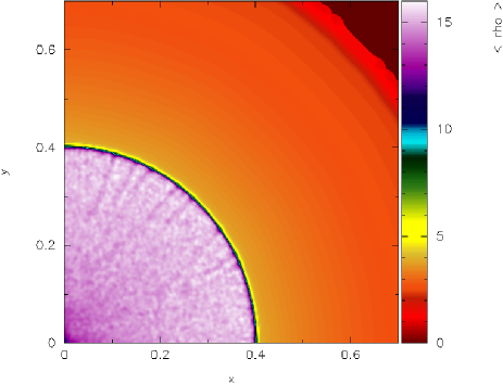
Figure 15: The Noh’s problem: density field in the first quadrant at $t=1.2$. All quantities are in code units. See text for details.

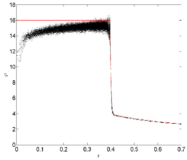
Figure 16: The Noh’s problem: density vs. radius relation for all particles at $t=1.2$. Solid line: theoretical expectation. All quantities are in code units. See text for details.

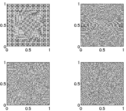
Figure 17: Positions of all particles at $t=0.02$ (top) and $t=2.7$ (bottom) for the two different initial configurations for the Gresho test: grid (left) and rings (right). All quantities are in code units. See text for details.

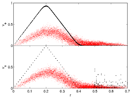
Figure 18: Initial (black dots) and final (red small points) azimuthal velocity profiles for the two Gresho tests: grid (top) and rings (bottom). All quantities are in code units. See the text for details.

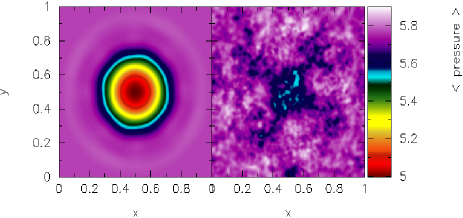
Figure 19: Initial ($t=0.02$, left) and final ($t=2.7$, right) pressure fields in the grid Gresho test. Note the increased pressure in the outskirts (white) and in the central regions of the vortex. All quantities are in code units. See the text for details.

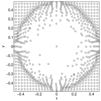
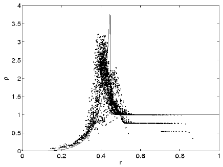
Figure 20: Top: spatial distribution of particles in a slice taken at z=0 and t=0.09 for the Sedov blast wave of test S1. Bottom: Radial density profile for the same test. Points: SPH particles; solid line: analytical prediction. All quantities are in code units.

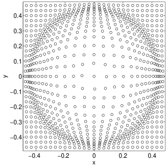
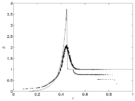
Figure 21: The same as in Fig. 20, but for the S2 test.

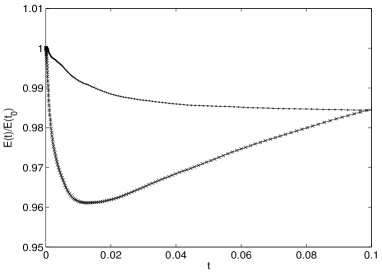
Figure 22: Energy conservations for Sedov test with artificial conductivity and variable viscosity. Points: with $\nabla h$ terms; crosses: without $\nabla h$ terms. All quantities are in code units.

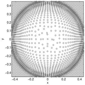
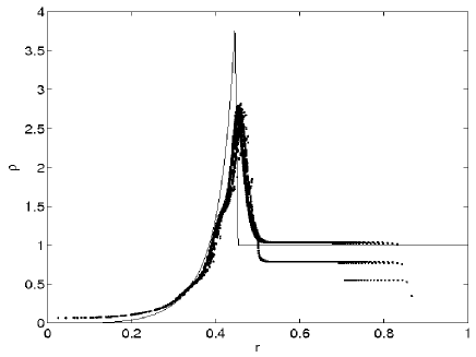
Figure 23: The same as in Fig. 20, but for the test S5.

Fig. 20 shows the $xy$ positions of particles belonging to the $z=0$ plane at $t=0.09$ for the S1 test, and the corresponding radial density profile, compared to the analytical expectation. A strong noise (which develops soon after the initial explosion) is evident in the particle positions, due to the huge unresolved discontinuity in thermal energy. The description of the shock evolution is quite poor, although its gross features are still captured.

Fig. 21 presents the same data for the S2 run, in which both the viscosity with variable $\alpha$ and artificial conduction are switched on. The increased precision in the description of the problem is immediately evident: the conductive term acts smoothing out the thermal energy budget of the central particle, strongly reducing the noise and allowing a symmetric and ordered dynamical evolution. The radial density profile (in which single particles, and not averages, are plotted) shows that the shock is well described. The density peak is a factor of $\sim 2$ lower than the analytical expectation, due to the intrinsic smoothing nature of the SPH technique.

Another test (S3) is carried dropping the $\nabla h$ correcting terms (see Sect. 3). While the differences in particle positions and density profiles are almost negligible, the comparison of the total energy conservations $E(t)/E(t_{0})$ in the two cases (Fig. 22) shows that the correction helps in containing losses due to wrong determinations of the gradient.

A fourth test (S4) is also run to check the behaviour of the individual time-stepping algorithm; the results are virtually indiscernible from the those of the previous case (not shown here). This is noteworthy as all particles must be “waken up” (using the method described in Sect. 4.2.1), being still and cold at the beginning of the simulation.

Finally, a test (S5) with increased numerical resolution is performed (Fig. 23). As expected, in this case, while the particles positions again accurately describe the evolution of the system, the shock boundary is sharper, and closer to the peak value of the analytical solution.

5.8 Self-gravitating collapse

The collapse of a gaseous self-gravitating sphere is another standard SPH 3-D test (Evrard 1988). The combined action of hydrodynamics and self-gravity leads the system, a sphere of gas initially far from equilibrium, with negligible internal energy and density profile $\rho\propto r^{-1}$, to a collapse in which most of its kinetic energy is converted into heat. An outward moving shock develops, a slow expansion follows and, at late times, a core-halo structure develops with nearly isothermal inner regions and the outer regions cooling adiabatically. To set the initial conditions, 10,000 particles of mass $1.25\times 10^{-2}M_{\odot}$ are placed in a sphere of radius $5\times 10^{-6}$ Mpc, in such a way that their initial density radial profile scales as $1/r$. Another sphere with 40,000 particles and consequently smaller particles’ masses (higher resolution) is also prepared. Two cases are examined: namely the collisionless collapse and the adiabatic collapse.

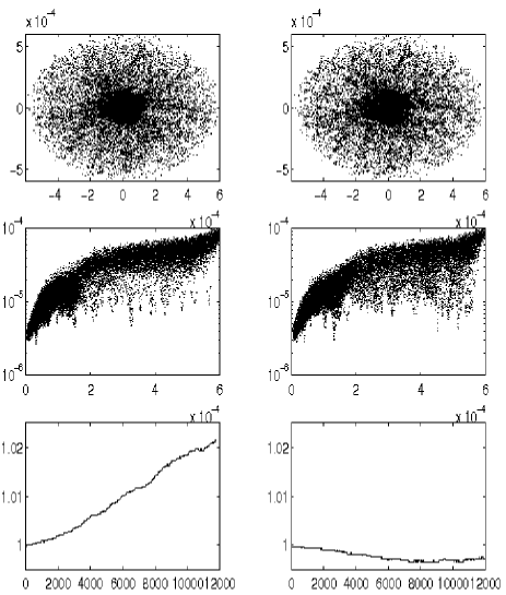
Figure 24: Collisionless collapse with adaptive softening lengths. Top: spatial distribution of particles projected onto the $xy$ plane after 12,000 steps; middle: softening lengths (code units) as a function of the radial coordinate; bottom: temporal conservation of the total energies of the systems $E(t)/E(t_{0})$, for the un-corrected (left) and corrected (right) tests.

5.8.1 Collisionless collapse

To check the performance of the adaptive softening length algorithm, tests are run switching off hydrodynamical interactions to mimic the collisionless collapse. A first case drops the hydrodynamical interactions, includes the adaptive softening algorithm but neglects the correcting terms presented in Section 2.1. It is meant to provide the reference case. The second one includes also the effects of these correcting terms.

Fig. 24 shows, in the upper panels, the spatial distribution of particles projected onto the $xy$ plane after during the collapse of the sphere, for the un-corrected (left) and corrected (right) cases: no evident difference is present. The same holds for (middle panels) the value of the softening lengths of particles as a function of the radial coordinate. However, the temporal conservation of the total energies of the systems $E(t)/E(t_{0})$ in the two cases are quite different (bottom panels of Fig. 24). If the correcting terms are not included a secular error in the energy conservation develops, reaching $2\%$, while the error is $\sim 10$ times smaller (albeit not completely eliminated) with the introduction of the extra-terms.

5.8.2 Adiabatic collapse

The standard hydrodynamical tests (Evrard 1988) are calculated with the following settings:

• E1 - constant softening lengths ($\epsilon_{i}=0.1R\times(m_{i}/M)^{0.2}$, with $R$ and $M$ total radius and mass of the sphere at the beginning of the simulation); Lagrangian SPH scheme, with constant viscosity ($\alpha=1$) and no artificial conduction;

• E2 - as E1, except for using adaptive softening lengths;

• E3 - adaptive softening lengths, viscosity with variable $\alpha$, and artificial conduction;

• E4 - as E3, higher resolution (40,000 particles).

The global energy trends are shown in Fig. 25, while Fig. 26 shows a magnification of the energy conservation $E(t)/E(t_{0})$ for the E1 and E2 runs. The energy conservation is always good, reaching a maximum error of $\sim 0.4\%$ at the moment of maximum compression. For comparison, in the same test the finite differences method by Evrard (1988) ensures conservation at $\simeq 1\%$, while Harfst et al. (2006) finds a maximum error of $\sim 3\%$ with a standard SPH implementation. Almost no difference can be noted between the variable and the constant $\epsilon$ runs, despite a variation of more than two orders of magnitude in the softening length values in the E2 run (see Fig. 27).

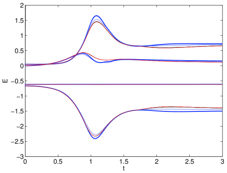
Figure 25: Energy trends in the cold collapse test. Light lines: red: test E1; black: test E2; blue: test E3. Heavy dotted blue line: test E4 (see text for details). Top to bottom: thermal, kinetic, total and potential energies. All quantities are in code units.

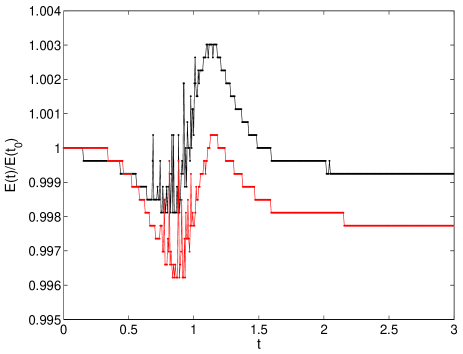
Figure 26: Magnification of the energy conservations $E(t)/E(t_{0})$ in the cold collapse tests. Black: testE1; red: testE2. See text for details.

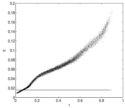
Figure 27: Softening lengths in the cold collapse test T2 at $t=0.8$. The solid line is the value of the constant softening length in test T1. All quantities are in code units.

The density and internal energy profiles at $t=0.8$, for the E1 to E3 runs, are shown in Fig. 28; the comparison between the E3 and the hi-res E4 runs is shown in Fig. 29 (the shock is moving outward leaving an inner, heated core). The discontinuity in density is smoothed out by the kernel smoothing, which in the current implementation requires a high number of neighbors ($\sim 60$), but the effects of the inclusion of the artificial conductive term are evident. We didn’t find any particular problem with the inclusion of the conductive term in a self-gravitating system.

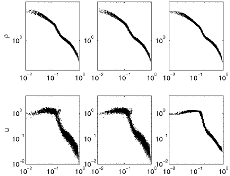
Figure 28: Density (top) and internal energy (bottom) profiles at $t=0.8$ in the cold collapse E1 (left), E2 (center) and E3 (right) tests. All particles are plotted.

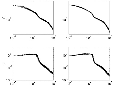
Figure 29: Comparison between cold collapse E3 (low-res, left) and E4 (hi-res, right) test: density (up) and internal energy (bottom) profiles at $t=0.8$.

We also run a X-SPH test, adopting $\eta=0.25$. While the energy trends are essentially identical to the ones the previous tests (not shown), the energy conservation is slightly worse, reaching an error of $\sim 2.5\%$. Indeed, Monaghan (2002) pointed out that a more complex treatment of the equations of motion should be adopted to achieve perfect energy conservation.

5.9 Isothermal collapse

Introduced by Boss & Bodenheimer (1979) and later revisited by Burkert & Bodenheimer (1993), the test on the isothermal collapse couples hydrodynamics and gravity, also adding rotation. It develops in a complex game of collapse and fragmentation. We run the test in the version proposed by Bate & Burkert (1997).

A homogeneous sphere of cold gas with initial radius $R=5\times 10^{16}$ cm and mass $M=1M_{\odot}$ is modelled retailing $\sim 78,000$ particles out of a uniform lattice. The sphere is put in solid body rotation around the $z$ axis, with angular velocity $\Omega=7.2\times 10^{-13}$ rad s^-1, and the otherwise flat density field is perturbed by $10\%$ in such a way that

$$\rho(\phi)=\rho_{0}[1+0.1cos(2\phi)],$$

where $\phi$ is the azimuthal angle about the rotation axis and $\rho_{0}=3.82\times 10^{-18}$ g cm^-3 (we achieve the density perturbation by varying the masses of particles instead of their positions). The gas is described by an isothermal equation of state, $P=c_{s}^{2}\rho$, with initial sound speed $c_{s}=1.66\times 10^{4}$ cm s^-1. It is assumed to be optically thin so that no mechanical heating can occur, and the adiabatic index is $\gamma=1.4$.

The test is very challenging and has been used to check the behaviour of both AMR and SPH codes. In particular, Bate & Burkert (1997) used it to study the effects of wrong calibrations of the smoothing and softening lengths in SPH (see Sect. 3.2). We run the test in four different cases:

• B1 - Lagrangian SPH with constant softening lengths ($\epsilon\simeq 5.26\times 10^{14}$ cm, an intentionally large value);

• B2 - Lagrangian SPH with adaptive softening lengths (no limits imposed on $\epsilon$ and $h$);

• B3 - as B2, but imposing a minimum smoothing and softening length $h_{min}=\epsilon_{min}=10^{14}$ cm, to avoid artificial clumping (as in Bate & Burkert 1997);

• B4 - as B2, with the X-SPH method (adopting $\eta=0.25$).

Figs. 30 to 33 plot the temporal evolution of the density field in the $z=0$ plane; shown are snapshots at $t=1.0$, $1.15$, $1.23$, and $1.26$, in units of free fall time, $t_{ff}=1.0774\times 10^{12}$ s. Fig. 34 plots the final density field at $t=1.29$ for the four tests. These plots can be compared to those by Bate & Burkert (1997) and Springel (2005).

The large value of $\epsilon$ assumed in the B1 test clearly demonstrates how a wrong choice of the softening length can result in catastrophic errors. The evolution of the system is clearly different from the grid solution used by Bate & Burkert (1997) as a proxy of the exact solution of the problem. Because of the excessive softening, clumps may be stable against collapse and a rotating structure forms, resembling a barred spiral galaxy. More realistic choices for $\epsilon$ may give better results, but the opposite problem (artificial clumping of unresolved structures) may arise in case of too small a softening length. Indeed, the case B2, in which the adaptive algorithm is adopted (note that $\epsilon=h$), gives much better results, but disorderly clumped sub-structures may form.

Imposing a minimum $\epsilon$ (=$h$, case B3) cures the problem (note however that the evolution of the system seems to be somewhat faster than the grid solution). Anyway, this prescription cannot be generalised. A more physically sounded solution may be the introduction of a pressure floor in unresolved regions, i.e. where the Jeans mass of the gas is not resolved by the SPH technique. This issue will be discussed in the forthcoming companion paper (Merlin et al. 2009, in preparation).

Finally, the X-SPH test B4 gives results that are essentially undiscernible from those of case B2, apart from a slightly less disordered density field in the regions surrounding the central collapsed structure.

Fig. 35 plots the temporal evolution of the maximum value of the density. This plot can be compared with Fig. 5a in Bate & Burkert (1997) and Fig. 12 in Springel (2005). The results for all tests are very similar and agree quite well with their SPH tests of comparable resolution (with the plateau at $\rho\simeq 2\times 10^{-15}$ g cm^-3 reached at $t=1.14$), except for the case B1 which clearly evolves faster.

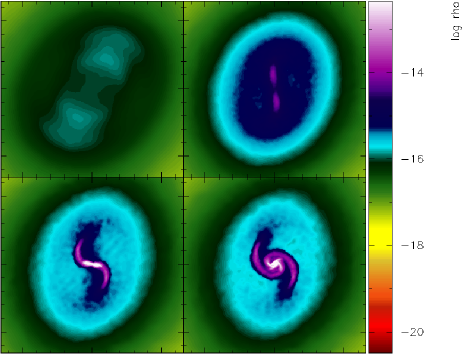
Figure 30: Evolution of the density field in the central region for the test B1. Plotted is the region within $1.54\times 10^{16}$ cm from the origin, on the $xy$ plane. Left to right, top to bottom: $t=1.0$, $1.15$, $1.23$, $1.26$, in units of free fall time, $t_{ff}=1.0774\times 10^{12}$ s.

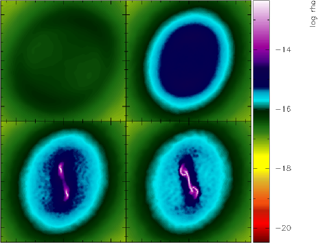
Figure 31: The same as in Fig. 30, but for test B2.

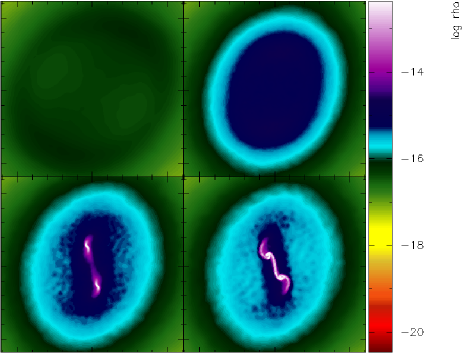
Figure 32: The same as in Fig. 30, but for test B3.

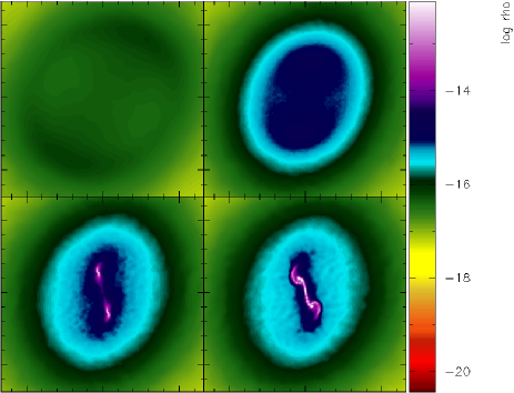
Figure 33: The same as in Fig. 30, but for test B4.

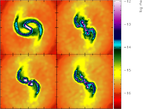
Figure 34: Final density field at $t=1.29$ (in units of free fall time) in the central region. Left to right, top to bottom: tests B1, B2, B3, B4. See text for details.

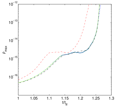
Figure 35: Maximum density in the isothermal collapse tests. B1: red dashed line; B2: green solid line; B3: blue thick dots; B4: black dot-dashed line. See text for details.

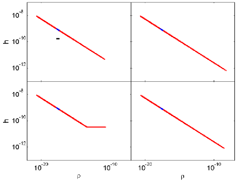
Figure 36: Initial (blue) and final (red) smoothing length $h$ of all particles in the four isothermal collapse tests (left to right, top to bottom: B1, B2, B3, B4). The softening length $\epsilon$ is equal to $h$ in the B2, B3 and B4 runs; the black dots in the top left panel show its constant value in the test B1. The abrupt truncation in the bottom left panel is due to the imposed $h_{min}$ ($=\epsilon_{min}$) in the test B3.

For reference, Fig. 36 shows the initial and final values of both $\epsilon$ and $h$ (which are equal in the cases B2, B3 and B4) as a function of $\rho$ in the four runs.

5.9.1 Parallel run

Finally, we re-computed the case B2 test using 16 parallel CPUs. Fig. 37 shows the comparison between the final density field for this run and for the original one with single CPU. Although the agreement is good, and no sign of a multi-processor subdivision of the domain is present, some differences in local morphological features are present; these are more evident looking at Fig. 38, where the comparison is made for the smoothing lengths values. While the gross features and the minimum and maximum values are very similar, differences in the local clumping of particles are clearly present.

We ascribe this flaw to the parallel Oct-Tree scheme. The global tree constructed by $N>1$ CPUs is slightly different from the one built by a single processor on the same spatial domain: the regions in which two or more different CPUs interact are described by a different cell architecture depending on $N$ (note that the reason for this is that the cells have to be always cubic; indeed, the problem should not occur if a binary tree, in which cells have adaptive shapes, was used). This causes a slightly different approximation of the gravitational force, due to the opening cell criterion, giving in turn a slightly different dynamical evolution.

To prove the validity of this speculation, we run again the same tests reducing the opening angle $\theta$ to $0.1$ instead of the standard 0.8. In this way, the approximation given by the adoption of the tree structure should become of negligible importance (at the expenses of a much longer computation time). Indeed, looking at Figs. 39 and 40, we can notice an improvement in that the density fields are more similar, although still not exactly identical. An ideal run with $\theta=0$ (i.e., exact particle-particle interaction) should give almost identical distributions of particles.

We must point out that this flaw may be of non-negligible importance when dealing with phenomena that directly depend on the local density field, such as the star formation and feedback processes. The same simulation run on a different number of CPUs may give slightly different results because of this issue.

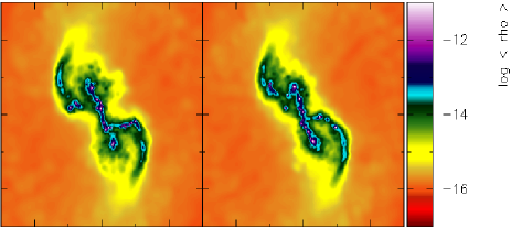
Figure 37: Comparison between the final density fields for a single CPU (left) and a 16 parallel CPUs (right) runs of the B2 test. See the text for details.

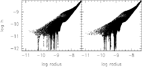
Figure 38: Comparison between the final $h$-radius relation, for a single CPU (left) and a 16 parallel CPUs (right) runs of the B2 test. See the text for details.

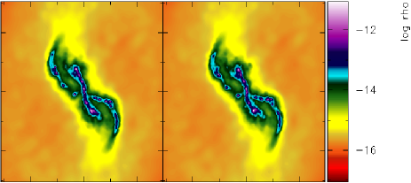
Figure 39: Comparison between the final density fields for a single CPU (left) and a 16 parallel CPUs (right) runs of the B2 test, in a run with tree opening angle $\theta=0.1$. See the text for details.

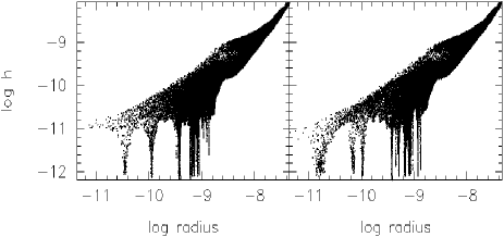
Figure 40: Comparison between the final $h$-radius relation, for a single CPU (left) and a 16 parallel CPUs (right) runs of the B2 test, in a run with tree opening angle $\theta=0.1$. See the text for details.

5.10 Collision of two gas spheres

The collision between two gaseous Plummer spheres is very crucial test for the energy conservation. The tests are run in 3-D, with adaptive softening lengths, variable $\alpha$ viscosity, and thermal conduction.

Each of the two spheres (of unit mass, unit radius, and negligible initial internal energy) are set up randomly selecting 10,000 particles in a way that their initial density radial profile resembles the Plummer profile, $\rho\propto(1+r)^{-5/2}$. Their centres are on the $x$ axis.

In a first run (C1) we follow a head-on collision, assigning a relative velocity of $1.5$ in the $x$ direction to the spheres. In a second run (C2) we added a shear component, giving relative velocities $|\Delta v_{x}|=0.15$ and $|\Delta v_{y}|=0.075$.

According to Hernquist (1993) the violent head-on collision of two polytropic stars does not conserve the energy within $\sim 10\%$. Modern formulations of SPH (see e.g. Rosswog & Price 2007) can handle the problem with much more accuracy, reducing the error below $0.1\%$.

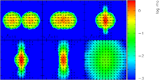
Figure 41: Evolution of the density field in the $z=0$ plane for the collision test C1. Left to right, top to bottom: $t=0.05$, $0.15$, $0.2$, $0.25$, $0.3$, $0.5$. Superposed is the velocity field.

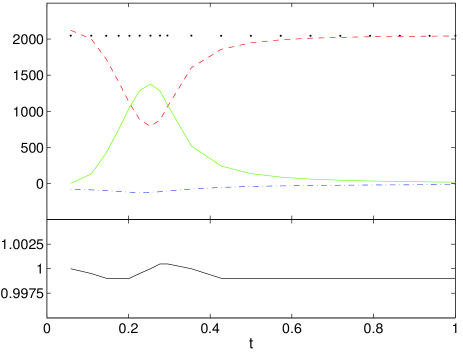
Figure 42: Top: energy trends in the collision test C1; black dots: total energy, blue dot-dashed line: potential, red dashed line: kinetic, green solid line: thermal. Bottom: magnification of the total energy conservation $E(t)/E(t_{0})$.

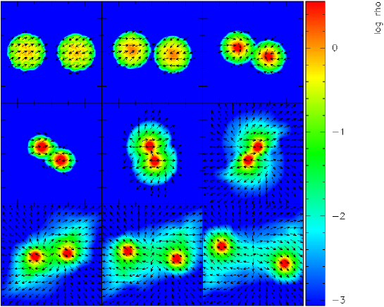
Figure 43: Evolution of the density field in the $z=0$ plane for the collision test C2. Left to right, top to bottom: $t=0.03$, $0.38$, $0.77$, $1.16$, $1.55$, $1.94$, $2.72$, $3.5$, $4.29$. Superposed is the velocity field.

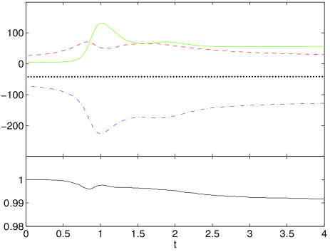
Figure 44: Top: energy trends in the collision test C2; black dots: total energy, blue dot-dashed line: potential, red dashed line: kinetic, green solid line: thermal. Bottom: magnification of the total energy conservation $E(t)/E(t_{0})$.

Figs. 41 and 43 plot the density and velocity fields at different times, on a slice taken at $z=0$. In our tests, the energy conservation is good (see Figs. 42 and 44), with a maximum error of $\sim 0.2\%$ in the head-on collision, and $\sim 1\%$ error when the shear component is added.

5.11 Two-components evolution

As a final test, we studied the evolution of a two-components fluid in order to investigate the behaviour of the adaptive smoothing and softening length algorithm in presence of more than one material. We set up two spheres of the same radius, $R=10^{3}$ pc, and mass, $M=4\times 10^{4}M_{\odot}$, using for each sphere the particle distribution adopted adiabatic collapse test by Evrard. One of the two systems was considered as made of collisionless bodies, with negligible pressure, thus mimicking the behaviour of a Dark Matter halo; the other one was instead considered as made of gas, with an initial temperature of 1000 K. The system was the let free to evolve under the action of self-gravity and hydrodynamical interactions, in four different runs with the following settings:

• TC1 - constant softening lengths, $\epsilon_{i}=0.1R\times(m_{i}/M)^{0.2}$; null initial velocities

• TC2 - adaptive softening lengths, null initial velocities

• TC3 - as TC2, with an initial solid body rotation $\Omega=2.5\times 10^{-17}$ rad s^-1, for both components

• TC4 - as TC3, but with counter-rotating initial tangential velocities (same magnitude).

While the collisionless component soon collapses under self-gravity, later reaching relaxation, the gas undergoes a phase of expansion because of its internal pressure, but in the central region, where it also interacts with collapsing Dark Matter, reaching very high densities.

The free expansion of a system of particles is by itself a demanding test, and a loss of total energy is a common flaw for Lagrangian codes. Furthermore, the rotation imposed in the last two runs makes the problem more complicated. In our tests, a further complication was given by the dynamical interaction within the central regions of the system, where the hydrodynamical pressure of the gas struggled against self-gravity and the (stronger) gravitational action of the collisionless component. Moreover, when the adaptive $\epsilon$ scheme was used, gas particles had to cope with a large variation of their interaction sphere, due to the presence of Dark Matter particles in the central regions, and to their absence in the outskirts, where in addition gas particles are far away from one another.

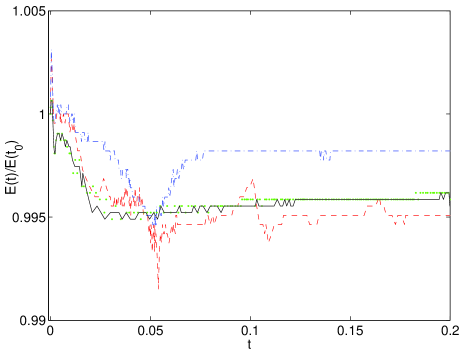
Figure 45: Two components test, energy conservation $E(t)/E(t_{0})$ for the four runs: dashed red line, TC1; blue dot-dashed line, TC2; green dots, TC3; black solid line, TC4.

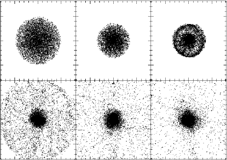
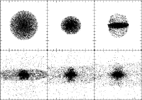
Figure 46: Two components test, case TC3. Dark Matter particles projected onto the $xy$ (top panels) and $xz$ (bottom panels) planes: left to right, top to bottom, $t=0.5$, 1.0, 1.5, 2.0, 2.5 Gyr.

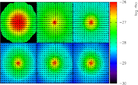
Figure 47: Two components test, case TC3. Gas density and velocity fields in a slice taken at $z=0$: left to right, top to bottom, $t=0.5$, 1.0, 1.5, 2.0, 2.5 Gyr.

Figure 48: Two components test: comparison between the central velocity fields in cases TC3 (left) and TC4(right), in a slice taken at $z=0$, at $t=2.5$ Gyr.

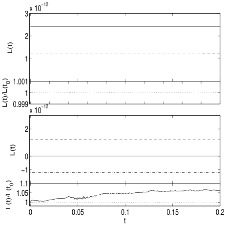
Figure 49: Two components test, angular momenta conservations. Top panels: test TC3, bottom panels: test TC4. Shown are the total (solid lines), gas (dashed lines) and Dark Matter (dash-dotted lines) angular momenta as a function of time $L(t)$, and conservations as a function of time $L(t)/L(t_{0})$ (same meaning of the symbols). Note that in the TC3 test the gas and Dark Matter lines are superposed because they have identical angular momentum.

Fig. 45 plots the energy trends for all the four tests. The conservation is very good in all cases, with a maximum error well below $1\%$; quite surprisingly, the worst performance is given by the constant $\epsilon$ scheme, while the corresponding test with adaptive softening performs better staying below a $\sim 0.5\%$ error.

Fig. 46 shows the evolution of the Dark Matter component in the test TC3, projected on the $xy$ and on the $xz$ planes (the case TC4 run gives almost undistinguishable plots). Clear is the early formation of a disk due to the initial rotational velocity, and a subsequent expansion which leaves a dense core with a loosely disky shape. On the other hand, the gas component expands with almost radial motion (Fig. 47), but in the central regions the interaction with the collisionless component plays an important role. Indeed, looking at Fig. 48 where a magnification of the velocity field in the central region at late times is shown for the tests TC3 and TC4, the difference in the two cases is clear: in the counter-rotation run the gas in the innermost zone has inverted its sense of motion and co-rotates with the Dark Matter, creating a complex pattern of velocities.

The conservation of angular momenta in the tests TC3 and TC4 is shown in Fig. 49. We find a maximum error of $\sim 6\%$ in the relative error for the total momentum in the counter-rotation test; in this case the absolute violation is anyway small because of the very small total initial momentum. In all the other cases the conservation is always very satisfactory.

6 Conclusions

We have presented the basic features of EvoL, the new release of the Padova parallel N-body code for cosmological simulations of galaxy formation and evolution. In this first paper, the standard gravitational and hydrodynamical algorithms have been extensively reviewed and discussed, as well as the parallel architecture and the data structures of the code. EvoL includes some interesting options such as adaptive softening lengths with self-consistent extra-terms to avoid large errors in energy conservation, $\nabla h$ terms in the SPH formalism, variable $\alpha$ viscosity formulation, and artificial thermal conduction terms to smooth out pressure at contact discontinuities.

We have also performed and presented an extended series of standard hydrodynamical tests to check the ability of the code to handle potentially difficult situations. The results are encouraging. Almost all tests have given results in nice agreement with theoretical expectations and previous calculations with similar codes, sometimes even showing better performance. In particular, we showed how the inclusion of an artificial thermal conduction term as suggested by Price (2008) significantly improves the modeling of demanding problems such as the Kelvin-Helmoltz instability or the Sedov-Taylor point-like explosion. Furthermore, the adoption of a variable softening lentghs algorithm allows for a higher degree of adaptivity without resulting in appreciable losses in terms of precision and conservation of energy. While some typical flaws of SPH codes are still present (e.g., problems in the conservation of vorticity because of spurious shear viscosity), these new features clearly improve the method and positively aid in curing well-known drawbacks of the SPH algorithm.

It must be however pointed out that the new features must be extensively tested, especially in situations of interest for cosmological simulations (i.e., gas dynamics in presence of a Dark Matter and/or stellar components). Here, we have restricted our analysis to standard hydrodynamical problems. Other and new tests will be presented in the companion paper by Merlin et al. (2009, in preparation), dedicated to the inclusion in EvoL of radiative cooling, chemical evolution, star formation, energy feedback, and other non-standard algorithms.

Appendix A $N$-dimensional kernel

The general form for the $N$-dimensional spline kernel function ($1\leq N\leq 3$) is

$$W_{N}(r,\epsilon)=\eta_{N}\times\begin{cases}\frac{2}{3}-u^{2}+\frac{1}{2}u^{3}&\text{if $0\leq u<1$,}\\ \frac{1}{6}(2-u)^{3}&\text{if $1\leq u<2$,}\\ 0&\text{if $u\geq 2$,}\end{cases}$$ (82)

where

$$\eta_{N}=\frac{1}{h^{N}}\times\begin{cases}1&\text{if N = 1,}\\ 15/(7\pi)&\text{if N = 2,}\\ 3/(2\pi)&\text{if N = 3.}\end{cases}$$ (83)

Derivatives are straightforwardly obtained from this expression. The 1-D and 2-D kernels have been used where necessary in some of the hydrodynamical tests presented in Sect. 5.

Appendix B Summary of equations of motion and conservation

Gravitational acceleration:

$$\frac{d\@vec{v}_{i,grav}}{dt} =$$

$$-\sum_{j}m_{j}\left[\frac{\phi_{ij}^{\prime}(\epsilon_{i})+\phi_{ij}^{\prime}(\epsilon_{j})}{2}\right]\frac{\@vec{r}_{i}-\@vec{r}_{j}}{|\@vec{r}_{i}-\@vec{r}_{j}|}$$

$$-\sum_{j}m_{j}\frac{1}{2}\left[\frac{\xi_{i}}{\Upsilon_{i}}\frac{\partial W_{ij}(\epsilon_{i})}{\partial\@vec{r}_{i}}+\frac{\xi_{j}}{\Upsilon_{j}}\frac{\partial W_{ij}(\epsilon_{i})}{\partial\@vec{r}_{j}}\right],$$

Hydrodynamical acceleration (for SPH particles only):

$$\frac{d\@vec{v}_{i,hyd}}{dt} = \sum_{j}m_{j}\times$$

$$\left[\frac{P_{i}}{\rho_{i}^{2}}\left(1+\frac{\zeta_{i}/m_{j}}{\Omega_{i}^{*}}\right)\nabla_{i}W_{ij}(h_{i})+\right.$$

$$\left.\frac{P_{j}}{\rho_{j}^{2}}\left(1+\frac{\zeta_{j}/m_{i}}{\Omega_{j}^{*}}\right)\nabla_{i}W_{ij}(h_{j})+\Pi_{ij}\bar{\nabla_{i}W_{ij}}\right],$$

Specific internal energy evolution (for SPH particles only):

$$\frac{du_{i}}{dt} =$$

$$\sum_{j}m_{j}\left[\frac{P_{i}}{\rho_{i}^{2}}\left(1+\frac{\zeta_{i}/m_{j}}{\Omega_{i}^{*}}\right)(\@vec{v}_{j}-\@vec{v}_{i})\cdot\nabla_{i}W_{ij}(h_{i})\right.$$

$$+\left.\left(\frac{1}{2}\Pi_{ij}+\Pi_{ij}^{u}\right)w_{ij}|\bar{\nabla_{i}W_{ij}}|\right].$$

In these expressions,

$$\Omega_{i}^{*}=1-\frac{\partial h_{i}}{\partial n_{i}}\sum_{j}\frac{\partial W_{ij}(h_{i})}{\partial h_{i}},$$ (87)

$$\Upsilon_{i}=\left[1-\frac{\partial\epsilon_{i}}{\partial n_{i}}\sum_{j}\frac{\partial W_{ij}(\epsilon_{i})}{\partial\epsilon_{i}}\right],$$ (88)

$$\xi_{i}=\frac{\partial\epsilon_{i}}{\partial n_{i}}\sum_{j}\frac{\partial\phi_{ij}(\epsilon_{i})}{\partial\epsilon_{i}},$$ (89)

and

$$\zeta_{i}=\frac{\partial h_{i}}{\partial n_{i}}\sum_{j}m_{j}\frac{\partial W_{ij}(h_{i})}{\partial h_{i}}.$$ (90)

The smoothing kernel $W$ is given by Eq. 4, whereas the softened gravitational potential $\phi$ is given by Eq. 2.1.

The standard equation of state is that of an ideal gas,

$$P=(\gamma-1)\rho u,$$ (91)

where $\gamma$ is the adiabatic index (5/3 for a monatomic gas); a more general equation of state will be presented in Merlin et al. (2009, in preparation).