Modeling Planetary System Formation with N-Body Simulations: Role of Gas Disk and Statistics Comparing to Observations

Abstract

During the late stage of planet formation when Mars-sized cores appear, interactions among planetary cores can excite their orbital eccentricities, accelerate their mergings and thus sculpture their final orbital architecture. This study contributes to the final assembling of planetary systems with N-body simulations, including the type I or II migrations of planets, gas accretion of massive cores in a viscous disk. Statistics on the final distributions of planetary masses, semimajor axes and eccentricities are derived, which are comparable to those of the observed systems. Our simulations predict some new orbital signatures of planetary systems around solar mass stars: $36\%$ of the survival planets are giant planets ($>10M_{\oplus}$). Most of the massive giant planets ($>30M_{\oplus}$) locate at 1-10AU. Terrestrial planets distribute more or less evenly at $<1-2$ AU. Planets in inner orbits may accumulate at the inner edges of either the protostellar disk (3-5 days) or its MRI dead zone (30-50 days). There is a planet desert in the mass-eccecntricity diagram, i.e., lack of planets with masses $0.005-0.08M_{J}$ in highly eccentric orbits $(e>0.3-0.4)$. The average eccentricity ($\sim 0.15$) of the giant planets ($>10M_{\oplus}$) is bigger than that ($\sim 0.05$) of the terrestrial planets ($<10M_{\oplus}$). A planetary system with more planets tends to have smaller planet masses and orbital eccentricities on average.

1 Introduction

To date, around 490 exoplanets have been detected, mostly by Doppler radial velocity measurements(e.g., see Udry & Santos 2007 for a review of their statistics). The masses of the planets range from order of Earth mass ($M_{\oplus}$) to tens of Jupiter masses ($M_{J}$). Among them, the most recently observed HD 10180 system records the most numerous planets in exoplanetary systems(Lovis et al. 2010). A study of multi-planet systems is helpful for understanding the formation history of planetary architecture due to planetary interactions (e.g., Wittenmyer et al. 2009). Recent statistics of single and multiple planetary systems have revealed several new possible signatures(Wright et al. 2009):

1. Including systems with long-term radial velocity trends, at least 28% of known systems appear to contain multiple planets. Thus multi-planet systems seem to be common.

2. The distribution of orbital distances of planets in multi-planet systems and single planets are inconsistent: single-planet systems show a pileup at period of $\sim 3$ days and a jump near 1 AU, while multi-planet systems show a more uniform distribution in log-period.

3. Planets in multi-planet systems have somewhat smaller eccentricities than single planets.

4. Exoplanets with their minimum masses bigger than Jupiter have eccentricities broadly distributed across $0<e<0.5$, while lower mass exoplanets exhibit a distribution peaked near $e=0$.

5. There may be a positive correlation between stellar masses and the occurrence rate of Jovian planets within 2.5AU (Johnson et al. 2007). This might be a reflection of the correlation of stellar masses with their circumstellar disks.

Concurrently, our theoretical insights into the process of planet formation have improved greatly. According to the conventional core accretion scenario, planets formed in circumstellar disks. Through sedimentation of dust and cohesive collisions of planetesimals, Mars-sized embryos will form through runaway and oligarchic growth (Safronov 1969, Kokubo & Ida 1998). Angular momentum exchanges between the embryos and the gas disk will cause a fast inward migration (type I) of the embryos in an isothermal disk(Goldreich & Tremaine 1979; Ward 1997; Tanaka et al. 2002). In some circumstance, for example, in a region that magnetorotation instability (MRI) is active (Laughlin et al., 2004, Nelson & Papaloizou 2004), or in a radiative disk (Paardekooper & Mellema 2006, Kley et al. 2009), the speed of type I migration can be greatly reduced or even with its direction being reversed. Thus the embryos can be effectively sustained. As long as they grow beyond some critical masses ($\sim 10M_{\oplus}$), quasi-hydrostatic gas sedimentation begins in the Kelvin-Helmholtz timescale (Pollack et al. 1996, Ikoma et al. 2000), which may last for million years until the final runaway gas accretion sets in. Type I migration of planetary cores is helpful to shorten the timescale of giant planet formation, provided a factor of $\sim 10$ reducing of the migration speed (Alibert et al. 2005). The newly formed giant planets then undergo type II migration before the gas disk is depleted.

According to the above scenario of single planet formation, planetary population synthesis has reproduced successfully most of the statistical characteristics for the observed systems. In a serious of works, Ida & Lin (2004a, 2004b, 2005 and 2008) predicted a planet desert with masses in 10-100 $M_{\oplus}$, due to the runaway gas accretion of giant planets, and confirmed the observed correlation that the planet detection rate increases with the metallically of their host star(Fischer & Valenti 2005). Other studies with population synthesis of planets, such as Kornet & Wolf (2006), Mordasini et al. (2009a,2009b), give more constrains of planet formation model based on observational data.

However, planets formed in an environment with many siblings. Perturbations from neighbor protoplanets may excite their eccentricities, which is helpful to planet formation in some cases. For example, the inward type II migration of gas giants in outside orbits may trap the planetary cores in inner mean motion resonances (mainly 2:1 resonance), thus results in their mergings into hot super-Earths (Zhou et al. 2005, Raymond et al. 2006). While planetary perturbations may inhibit the core growth in other cases, e.g., the lack of planets in the location of asteroid belt may be due to Jupiter perturbations. Moreover, planet-planet scattering is thought as the major cause for the eccentricities of the observed planetary systems (Rasio & Ford 1996, Zhou et al. 2007, Chatterjee et al. 2008, Juri$\acute{c}$ & Tremaine 2008). Planet population synthesis method without including the planet-planet scattering procedure is incomplete to account for the observed planetary signatures.

By taking the planet-planet scattering effect into consideration, N-body integration of the full planetary equations is necessary. Based on N-body simulations and a self-consistent disk evolution, Thommes et al. (2008) investigated the formation of giant planets in the context of disk evolution, and revealed some interesting tendencies that relate the planetary systems with their birth disks. Ogihara & Ida (2009) studied the formation and distribution of terrestrial planets around M dwarf stars, and find the final configurations of planets depend on the speed of type I migration.

In this work, we employ the N-body method to study the final assembly of planetary systems. The aims of this study are twofold: (1) to explain the observed statistics of planet masses and orbit parameters, thus to constrain the parameters that are most suitable for planet formation; (2) to guide the future observation by extending our study to the mass regime that is not yet detectable. We adopt the standard model of core accretion scenario, which includes the standard type I and II migrations of planets.

For N-body simulations of planetary formation and evolution, one of the major difficulties is the initial conditions of planetary embryos and the embedded protoplanetary disk. At the later stage of planet formation, most of the embryos are assumed to be formed with their masses ranging from Mars to several Earths (or even bigger). However, their radial distributions are quite uncertain. Also, the parameters of viscous disks (their extensions, surface density distributions, depletion timescales, etc.) are quite uncertain. These parameters may be coupled, and their effects are different. As shown in Thommes et al. (2008), disk properties play a key role in determining the planetary migration. They chose the mass and the viscosity of the protostellar disk as two free parameters. To simplify the model used in this paper, through some tests, we fix most of the parameters to some fiducial values, except letting the gas disk depletion timescale ($\tau_{disk}$) and disk mass ($\Sigma_{g}$) as two free parameters. The effects of other parameters on the final architecture of the planetary systems are also discussed.

The arrangement of this paper is as follows. First we describe the model and method of the paper in §2,. Then some analytical estimation about the orbital configuration under type I and II migrations is given in §3. The effects of disk parameters on the evolution and final architecture of the planetary systems are discussed in §4. In §5 , the distributions of planet parameters (masses, semimajor axes, eccentricities) from simulations are compared with observations. To see if our results are credible in two-dimensional model , we survey the differences in three-dimensional model in §6. The conclusions are presented in §7, with discussions and some implications for future works.

2 Model and Initial Setup

Our investigation starts at the stage that most of the planetary embryos have cleared up their feeding zones and obtained their isolation masses. This may correspond to an epoch of $\sim 1$ Myr after the birth of the protostar. Embryos in inner obits might undergo type I migration, which is assumed to be stalled at some locations such as the inner edge of MRI dead zone of the gas disk (Kretke & Lin 2007, Kretke et al. 2009). For embryos outside the snow line, some of them are large enough (several $M_{\oplus}$) for the onset of efficient gas accretion. They begin to accrete gas, open gaps, and undergo type II migration. Detailed model and parameters that we used in this paper are presented as follows.

2.1 Viscous Disks

Pre-main-sequence stars accrete gas through circumstellar disks. Although the origin of the disk viscosity is still in controversial, the onset of MRI helps to the transportation of angular momentum through the disk (Balbus & Hawley 1991). In this paper, we adopt the ad hoc $\alpha$-prescription (Shakura & Sunyaev 1973) to model the effect of mass transportation during the stage of classical T-Tauri stars. In such a disk, the kinematical viscosity is expressed as $\nu=\alpha c_{s}h$, where $c_{s}$ and $h$ are the sound speed in mid-plane disk and the density scale height, respectively(Table 1). The surface density at stellar distance $a$ is given as (e.g., Pringle 1981),

$$\Sigma_{g}=\frac{\dot{M}}{3\pi\alpha c_{s}h}\left[1-\left(\frac{R_{*}}{a}\right)^{1/2}\right],$$ (1)

where $\dot{M}$ is the gas accretion rate and $R_{*}$ is the stellar radius. For a T-Tauri disk with stellar mass of $0.2M_{\odot}\leq M_{*}<2.0M_{\odot}$, the observed accretion rate is (Natta et al. 2006, Vorobyov & Basu 2009)

$$\dot{M}=2.5\times 10^{-8}M_{\odot}{\rm yr}^{-1}\left(\frac{M_{*}}{M_{\odot}}\right)^{1.3\pm 0.3}.$$ (2)

In an optically thin disk, adopting the parameters in Table 1 and let $a\gg R_{*}$, we get Eq.(3) from equation (1),

$$\Sigma_{g}=2400{\rm~{}g~{}cm^{-2}}\left(\frac{\alpha}{10^{-3}}\right)^{-1}\left(\frac{M_{*}}{M_{\odot}}\right)^{0.8}\left(\frac{a}{1\rm~{}AU}\right)^{-1}.$$ (3)

For an $\alpha$-disk with constant $\alpha=10^{-3}$, we derive the minimum mass solar nebular (MMSN) except with a different slope, $\beta=-\ln\Sigma_{g}/\ln a$ (c.f., $\beta=3/2$ in MMSN, Hayashi 1981,Ida & Lin 2004a). We also assume that the protoplanetary disk has a layered structure as a sandwich: inside a location $a_{\rm crit}$, the protostellar disk is thermally ionized partly, while outside $a_{\rm crit}$ only the surface layer is ionized by stellar X-rays and diffuse cosmic rays, leaving the central part of the disk a highly neutral and inactive “deadzone”(Gammie 1996). The viscosity in the MRI active region could be one or two magnitudes larger than that of the dead zone(Sano et al. 2000). By assuming a constant accretion rate across the disk at a specific epoch in equation (1), a positive density gradient is expected near $a_{\rm crit}$, which helps to halt the embryos under type I migration(Kretke & Lin, 2007, Kretke et al. 2009).

To model this effect, we let $\alpha_{\rm MRI}$ and $\alpha_{\rm dead}$ denote the $\alpha$-values of the MRI active and dead regions, respectively. The effective $\alpha$ for the disk is modeled as (Kretke & Lin, 2007):

$$\alpha_{\rm eff}(a)=\frac{\alpha_{\rm dead}-\alpha_{\rm MRI}}{2}[{\rm erf}(\frac{a-a_{\rm crit}}{0.1a_{\rm crit}})+1]+\alpha_{\rm MRI},$$ (4)

where ${\rm erf}$ is the error function, $0.1a_{\rm crit}$ is thought as the width of the transition region. In this paper, we adopt $\alpha_{\rm MRI}=0.02,\alpha_{\rm dead}=10^{-4}$ (Sano et al. 2000). The small value of $\alpha_{\rm dead}$ is adopted to obtain a reasonable timescale of type II migration (see Eq.[16] later). Alternative choices of $\alpha_{\rm dead}$ are also discussed in §4.1.

The location of the inner edge of the MRI dead zone, $a_{\rm crit}$, varies with the disk temperature, kinematics and mass accretion rate, etc. Here we adopt the expression from Kretke et al. (2009),

$$a_{\rm crit}=0.16~{}{\rm AU}(\frac{\dot{M}}{10^{-8}M_{\odot}{\rm yr}^{-1}})^{4/9}(\frac{M_{*}}{M_{\odot}})^{1/3}(\frac{\alpha_{\rm MRI}}{0.02})^{-1/5}.$$ (5)

During the evolution of a T-Tauri star and its disk, $\dot{M}$ decreases from $\leq 10^{-6}$ to $\sim 10^{-9}$ $~{}{\rm M}_{\odot}$ yr^-1, according to the infrared excess observation(e.g. Gullbring et al. 1998). So the location of $a_{\rm crit}$ is migrating inward as time proceeds. To simplify the procedure, we let the gas disk depletes uniformly in a timescale $\tau_{\rm disk}$, so $\dot{M}=\dot{M}_{0}\exp(-t/\tau_{\rm disk})$. Assuming a disk mass of $0.02M_{\odot}$ (Andrews & Williams 2005), we obtain $\dot{M}_{0}=0.02M_{\odot}/\tau_{\rm disk}$.

Substituting the previous equations (4) and (5) into equation (3), we obtain the following surface density for the circumstellar disk:

$$\Sigma_{g}=\Sigma_{0}f_{g}(\frac{a}{\rm 1AU})^{-1}(\frac{\alpha_{\rm eff}}{10^{-4}})^{-1}(\frac{M_{*}}{M_{\odot}})^{4/5}\exp({-\frac{t}{\tau_{\rm disk}}}),$$ (6)

where $f_{g}$ is the gas enhancement factor, $\Sigma_{0}=280$g cm^-2 is adopted in this work so that the total mass of the disk up to 100 AU is $0.02M_{\bigodot}$ for $f_{g}=1$, corresponding to the average disk mass in Taurus-Auriga star formation region(Beckwith & Sargent 1996). For such a disk, the Toomre’s criterion for the onset of gravitational instability is expressed as $Q=\frac{c_{s}\Omega_{K}}{\pi G\Sigma_{g}}=340(a/1AU)^{-3/4}f_{g}^{-1}$. So $Q>1$ holds and gravitational instability will not occur up to $100$ AU as long as $f_{g}\leq 10$.

We truncate the inner disk at the disk cavity due to the stellar magnetic field. Around the corotation radius, the stellar magnetic torque acts to extract angular momentum from the disk and spins down disk material. At the location where the stellar magnetic field completely dominates the disk internal stresses, sub-Keplerian rotation leads to a free-fall of disk material onto the surface of the star in a funnel flow along magnetic-field lines, which results in an inner disk truncationKönigl (1991). The maximum distance of the disk truncation is estimated at $\sim 9$ stellar radii. Considering that the radius of protostar is generally 2-3 times larger than their counterparts in the main sequence stage, the inner disk truncation would occur at $<0.1$AU. Thus we set the inner edge as 0.05AU in this paper.

2.2 Isolated Embryos and Type I Migration

According to the core accretion scenario of planet formation, planetary embryos form through cohesive collisions of heavy elements near the midplane of the circumstellar disk. Within the solid disk an embryo will grow until it accretes all the dust material round its feeding zone so that an isolation body is achieved (Kokubo & Ida 1998,Kokubo & Ida 2002). At the later stage of planet formation, inward migration of planetesimals under gas drag and planetary embryos under type I migration may change the distribution of embryos, which results in an uncertainty of the initial embryos masses. On the other hand, the MMSN model for the solid disk was derived according to the final solid masses of the present planets in the solar system (Hayashi 1981, Ida& Lin 2004a), which reflects the final distribution of the embryo, so we adopt the isolation masses with distribution as that of MMSN but with an enhancement factor $f_{d}=f_{g}$. In a gas disk, the instability of the isolation masses is suppressed until the gas disk is depleted. Assume the dynamical instability timescale of a group of isolated masses is the same as the disk dispersal timescale, the isolation masses are correlated with their mutual separations, and are given by (Kokubo & Ida 2002, Zhou et al. 2007)

$$M_{iso}=0.16M_{\oplus}~{}(f_{d}\eta_{\rm ice})^{3/2}(\frac{a}{1AU})^{3/4}(\frac{M_{*}}{M_{\bigodot}})^{-1/2}\left(\frac{k_{\rm iso}}{10}\right)^{3/2},$$ (7)

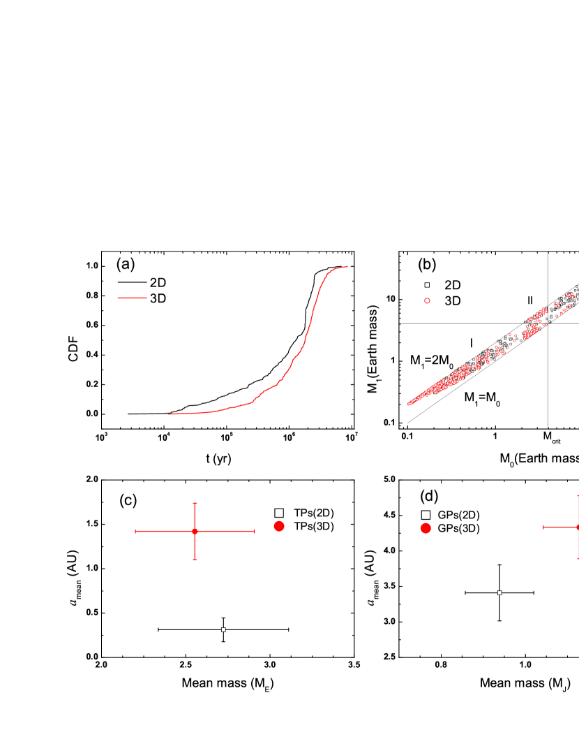
Figure 11: (a) The cumulative distribution function(CDF) of collision time. (b) The masses of embryos before collisions $M_{0}$ and the masses after collisions $M_{1}$.(c) & (d): Mean semimajor axis and mass for TPs and GPs respectively. In panel (c): $M_{\rm mean}=2.72M_{\oplus},a_{\rm mean}=0.31$AU (2D) and $M_{\rm mean}=2.55M_{\oplus},a_{\rm mean}=1.42$AU (3D) for TPs. In panel (d): $M_{\rm mean}=0.94M_{J},a_{\rm mean}=3.41$AU (2D) and $M_{\rm mean}=1.13M_{J},a_{\rm mean}=4.33$AU (3D) for GPs.

where $f_{d}$ is the heavy elements enhancement factor over MMSN model, $\eta_{\rm ice}=1$ inside $a_{\rm ice}$ and $4.2$ outside $a_{\rm ice}$, with $a_{\rm ice}$ the location of the snow line, beyond which water is condensed as ice from disk gas ($T\simeq 170K$). $k_{\rm iso}$ is the separation of embryos scaled by $R_{H}=(2M_{\rm iso}/3M_{*})^{1/3}a$. For $\tau_{\rm disk}=1-10$ Myr, $k_{\rm iso}=8-10$ at 1AU and $7-9$ at 10 AU for a disk with $f_{d}=1$ (See Fig.11 of Zhou et al. 2007 and details therein).

Due to the variation of the disk accretion rate and stellar radiation at different epoch of the protostar, the location of snow line varies (Garaud & Lin 2007). For a star with mass $\leq 3~{}M_{\odot}$, we adopt the snow line location as Kennedy & Kenyon (2008):

$$a_{ice}=2.7~{}{\rm AU}(\frac{M_{*}}{M_{\odot}})^{4/9}(\frac{\dot{M}}{10^{-8}M_{\odot}~{}{\rm yr}^{-1}})^{2/9}.$$ (8)

To model the type I migration of the embryos, we adopt the expression of the migration timescale from Cresswell & Nelson (2006), which is also valid for eccentric orbits,

$$\tau_{\rm mig,I} = -\frac{1}{C_{1}}\frac{1}{2.7+1.1\beta}\left(\frac{M_{*}}{M_{p}}\right)\left(\frac{M_{*}}{\Sigma_{g}a^{2}}\right)\left(\frac{h}{r}\right)^{2}$$ (9)

$$\left|\frac{1+(\frac{er}{1.3h})^{5}}{1-(\frac{er}{1.1h})^{4}}\right|\Omega^{-1},$$

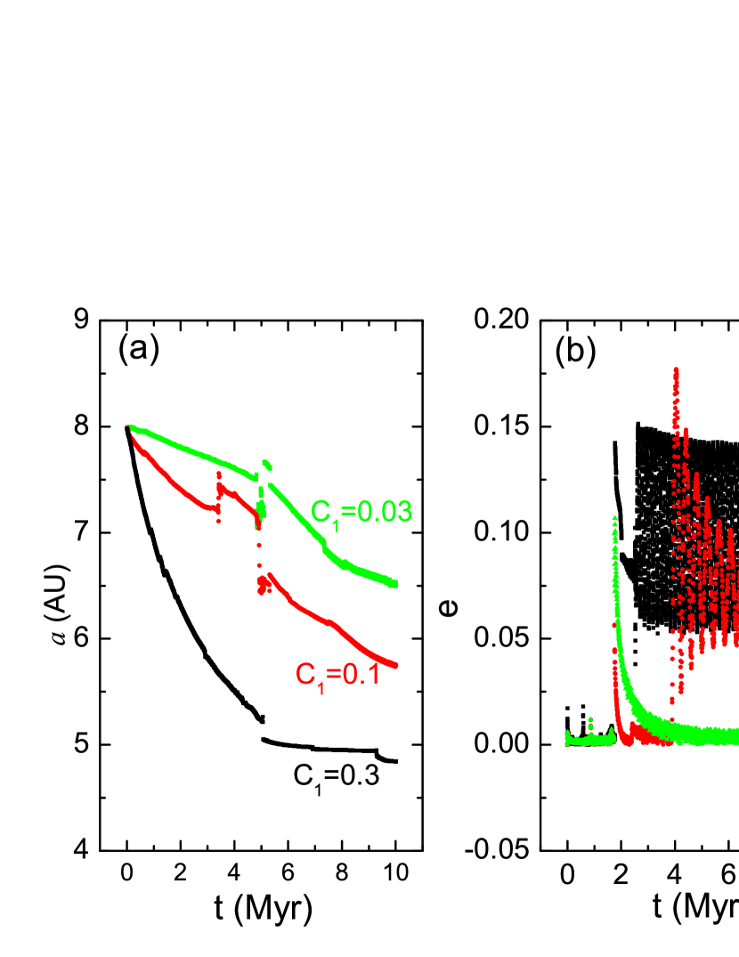
Figure 1: Some tests are run to determine the appropriate values of type I migration reduction factor $C_{1}$ in Eq.(9) and the eccentricity-damping rate $K$ in Eq.(17). (a) Migrations of a planet under different $C_{1}$ . (b) Eccentricity evolutions of a planet under different $K$ .

where negative (positive) value of $\tau_{\rm mig,I}$ corresponds to the inward(outward) migration respectively, $M_{p}$, $r$, $e$, $\Omega$ are the mass, position, eccentricity, angular velocity of the planet, respectively. Due to the MRI effect, $\beta\equiv-\partial{\rm ln}\Sigma_{g}/\partial{\rm ln}a$ can be negative near the location of maximum pressure $a_{\rm crit}$. $C_{1}$ is a reduction factor. Lots of literatures have shown that, to produce the observed planetary occurrence rate, $C_{1}\in[0.03,0.3]$ is an appropriate range (e.g. Alibert et al. 2005, Ida & Lin 2008). To test its validity in our model, we set $C_{1}=0.03,0.1,0.3$ and execute some test runs. As shown in Fig.1a, both the choice of $C_{1}=0.03$ and $0.1$ produce a very slow planet migration embedded in our disk model, which may result in the formation of hot Jupiters very difficult. So we set $C_{1}=0.3$ throughout this paper.

The presence of the gas disk will damp the eccentricities of embedded embryos(Goldreich & Tremaine 1980). The $e$-damping timescale can be described as (Cresswell & Nelson 2006),

$$\tau_{\rm edap,I}=\frac{Q_{e}}{0.78}\left(\frac{M_{*}}{M_{p}}\right)\left(\frac{M_{*}}{a^{2}\Sigma_{g}}\right)\left(\frac{h}{r}\right)^{4}\left[1+\frac{1}{4}(e\frac{r}{h})^{3}\right]\Omega^{-1},$$ (10)

where $Q_{e}=0.1$ is a normalization factor to fit with the hydrodynamical simulations.

2.3 Giant planet formation: gap opening and type II migration

According to the conventional accretion scenario, giant planets form through three major stages(Perri & Cameron 1974; Mizuno 1980; Pollack et al. 1996) : (1) Embryo growth stage. Protoplanetary cores form and grow mainly by the bombardment of planetesimals before they attain isolation masses. (2) Quasi-hydrostatic sedimentation stage. The accretion of planetesimals tapers as their supply in the feeding zone is depleted. This induces a quasi-hydrostatic sedimentation and the growth of the gaseous envelope due to the loss of entropy. (3) Runaway gas-accretion stage. When the mass of gas envelop becomes comparable to that of the core, a runaway stage of gas accretion sets in continually until the gas supply is exhausted by either the formation of a tidally induced gap near the protoplanet orbit or the depletion of the entire disk.

Through quasi-static evolutionary simulations, Ikoma et al. (2000) derived the critical core mass where significant gas accretion occurs:

$$M_{\rm crit}\sim 7M_{\oplus}\left(\frac{\dot{M}_{\rm core}}{10^{-7}M_{\oplus}{\rm yr}}\right)^{0.25}\left(\frac{\kappa}{1~{}{\rm cm^{2}~{}g}^{-1}}\right)^{0.25},$$ (11)

where $\dot{M}_{\rm core}$ is the rate at which planetesimals are accreted onto the core, and $\kappa$ is the grain opacity (see also Rafikov 2006). Due to the uncertainty of $\dot{M}_{\rm core}$ and $\kappa$, we assume $\dot{M}_{\rm core}\propto f_{g}$ and adopt $M_{\rm crit}=4M_{\oplus}f_{g}^{0.25}$ in this paper. A planet core beyond this critical mass will begin to accrete gas in a Kelvin-Helmholtz timescale, $\tau_{\rm KH}\simeq 10^{9}{\rm~{}yr}(M_{p}/M_{\oplus})^{-3}$, so that $dM_{p}/dt\simeq M_{p}/\tau_{\rm KH}$(Ikoma et al. 2000). However, the accretion rate is also limited by the replenishing rate of the materials ($\dot{M}_{\rm disk}$), so the accretion rate of the planetary embryos is expressed as(Ida & Lin 2004),

$$\frac{dM_{p}}{dt}=\min\left[10^{-9}(\frac{M_{p}}{M_{\oplus}})^{4}M_{\oplus}{\rm yr}^{-1},\dot{M}_{\rm disk}\right].$$ (12)

When the planet mass grows to sufficiently large, a tidal-induced gap in the gas disk forms around its orbit (Lin & Papaloizou 1979). The critical mass for gap-opening is determined by equating the timescale for Type I torques to open a gap (in the absence of viscosity) with that for viscous diffusion to fill it in. This gives (Armitage & Rice, 2005)

$$\frac{M_{p}}{M_{*}}\geq\alpha_{\rm eff}^{1/2}(\frac{h}{a})^{2}.$$ (13)

With $\alpha_{\rm eff}\sim 10^{-4}$ in the MRI dead zone, the critical mass is given by:

$$M_{I,II}=7.5(\frac{a}{\rm 1~{}AU})^{1/2}(\frac{M_{*}}{M_{\bigodot}})M_{\oplus}.$$ (14)

After the giant planet opens a gap around the disk, it is embedded in the viscous disk and undergos type II migration. As the mass of the planet grows and becomes comparable to the disk mass, migration slows down and eventually stops. The migration speed with the slow down effect can be expressed as(Alibert et al. 2005):

$$\frac{da}{dt}=-\frac{3\nu}{2a}\times\min(1,\frac{2\Sigma_{g}a^{2}}{M_{p}}).$$ (15)

So the migration timescale is given as:

$$\tau_{\rm mig,II} = 0.6{\rm~{}Myr}~{}(\frac{\alpha_{\rm eff}}{10^{-4}})^{-1}(\frac{a}{\rm 1AU})(\frac{M_{*}}{M_{\odot}})^{-1/2}$$ (16)

$$\ max(1,\frac{M_{p}}{2\Sigma_{g}a^{2}}).$$

During the migration of the giant planets, their eccentricities will be damped by the disk tide(Goldreich & Tremaine, 1979, 1980; Ward 1988), unless the planet is very massive ($\sim 20~{}M_{J}$, Papaloizou et al. 2001). As the $e$-damping rate due to the gas disk is quite elusive for different mass regimes of the planets, we adopt an empirical formula for the $e$-damping timescale (Lee & Peale 2002)

$$\tau_{\rm edap,II}=\tau_{\rm mig,II}/{\rm K},$$ (17)

where $K$ is a positive constant with a value ranging $10-100$. To choose an appropriate value of $K$, we execute some test runs with $K=10,30,100$. As shown in Fig.1b, the planet eccentricity is damped very quickly with $K=100$. For $K=30$, the eccentricity can be excited and effectively damped at the end of simulation when the gas disk has been nearly depleted. Therefor we take $K=10$ so that some planets in eccentric orbits can finally survive according to the observations.

The gas accretion of a planet will stop when all the gas material around the feeding zone($R_{H}=h$) is exhausted, this gives the truncation mass of a gas giant:

$$M_{\rm g,iso}(a)=120(\frac{a}{1AU})^{3/4}(\frac{M_{*}}{M_{\odot}})M_{\oplus}.$$ (18)

This limits the mass of a giant planet by pure gas accretion. However, collision and cohesive mergings may increase the masses of giant planets up to several Jupiter masses.

2.4 Equation of Motion

Based on the model described above, we investigate the late stage formation of the planetary system in this paper. The stellar mass is taken as $1~{}M_{\odot}$. The gas disk is assumed as in Equations (6). We further assume that embryos have obtained their isolated masses (see Eq.[7]) with $f_{d}=f_{g}$. We ignore those embryos with mass $\leq 0.1~{}M_{\oplus}$ in the inner and outer orbits, so that there are totally $38\sim 44$ isolated embryos initially in circular and coplanar orbits in [0.5-13.5]AU for a system with a gas and a solid disk $f_{g}=f_{d}=1$. The isolation masses and their radial extension will be changed accordingly for different $f_{g}=f_{d}$. The outer boundary of embryos is set according to the rule that, beyond which the core masses that can grow within 5 Myrs are less than 0.1 $M_{\oplus}$, according to the standard core growth (Kokubo & Ida 2002, Ida & Lin 2004a). Although this simplification may neglect their dynamical frictions to inner massive cores, this effect is similar to the damping effect by the gas disk tide, which is more effective and included already in our simulations.

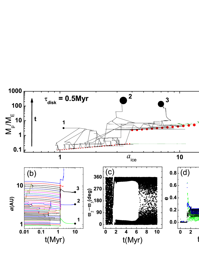
Figure 2: Evolution of orbits in a typical run that two of the three survival planets passed through a periastron alignment. Initially 44 embryos are put with a disk depletion timescale $\tau_{disk}=0.5$ Myr. Three planets are survival with masses $3.1M_{\oplus}$, $238.2M_{\oplus}$, $137.6M_{\oplus}$, and semimajor axes 1.07AU, 3.38AU, 6.98AU, respectively. (a)Planet growth and evolution in mass-semimajor axis plane. The red dots are the initial locations of the embryos. The green dots are those with either $a>50$AU or $e>1$ (being scattered out) during the evolution. (b) Evolution of semimajor axes of all embryos. (c) Evolution of periastron alignment angle ($\varpi_{2}-\varpi_{3}$). (d) Evolution of eccentricities for the three survival planets.

The angle elements (longitude of periastron, mean motion) of the embryos are randomly chosen. Fig.2 shows an example of the masses and initial locations of the embryos. According to equation (7), different $\tau_{\rm disk}$ gives slightly different values of $k_{\rm iso}$ and $M_{\rm iso}$(see Zhou et al. 2007).

The acceleration of an embryo with mass $M_{i}~{}(i=1,...N)$ is given as,

$$\frac{d}{dt}\textbf{v}_{i} = -\frac{G(M_{*}+M_{i})\textbf{r}_{i}}{r_{i}^{3}}+\sum_{j\neq i}^{N}GM_{j}\left[\frac{\textbf{r}_{j}-\textbf{r}_{i}}{|\textbf{r}_{j}-\textbf{r}_{i}|^{3}}-\frac{\textbf{r}_{j}}{r_{j}^{3}}\right]$$ (19)

$$\ -\frac{{\bf v}_{i}}{2\tau_{\rm mig}}-\frac{(\textbf{v}_{i}\cdot\textbf{r}_{i})\textbf{r}_{i}}{r_{i}^{2}\tau_{edap}},$$

where $\textbf{r}_{i}$ and $\textbf{v}_{i}$ are the position and velocity vectors of $M_{i}$ relative to the star, the third and fourth terms in the r.h.s. of the equation are the accelerations that cause the eccentricity damping and migration, respectively. For embryos with $M_{i}<M_{I,II}$ defined in Eq.(14), $\tau_{\rm mig}=\tau_{\rm mig,I}$ (Eq.[9]) and $\tau_{\rm edap}=\tau_{\rm edap,I}$ (Eq.[10]) are used. For those with $M_{i}>M_{I,II}$, $\tau_{\rm mig}=\tau_{\rm mig,II}$ (Eq.[16]) and $\tau_{\rm edap}=\tau_{\rm edap,II}$ (Eq.[17]) are used instead. Note that, during the growth of an embryo, it may cross the critical mass $M_{I,II}$, thus pass from type I to type II migration, and also the eccentricity-dampping mode is switched.

In the absence of mutual planet perturbations ($M_{j}=0,~{}j\neq i)$, i.e., without second term in the r.h.s. of Eq.(19), the secular variations of orbital elements for the embryo $M_{i}$ under migration and eccentricity-damping are derived from the classical perturbation theory:

$$\begin{array}[]{l}\left<\frac{da}{dt}\right>=-\frac{a}{\tau_{\rm mig}}-\frac{2e^{2}}{\tau_{\rm edap}(1+\sqrt{1-e^{2}})},\\ \left<\frac{de}{dt}\right>=-\frac{e(1-e^{2})}{\tau_{\rm edap}(1+\sqrt{1-e^{2}})},\\ \left<\frac{d\omega}{dt}\right>=0\end{array}$$ (20)

where $\omega$ is the argument of periastron of the embryo orbit.

3 Planet Configurations Under Migrations: Analytical Considerations

Before we present the numerical results, it will be useful to investigate some ideal cases that some cores undergo type I or II migrations only, and to see the configuration of the system without considering their mutual perturbations. This will be helpful to understand the onset of instability for the full system.

3.1 Planetary core configurations under type I migration

Suppose there are N planet cores with masses below $M_{I,II}$ so that they undergo type I migration. Eq.(9) gives $\tilde{a}/\dot{\tilde{a}}=\tau_{\rm mig,I}=k\tilde{M}_{p}^{-1}\tilde{a}\exp(t/\tau_{disk})$ for $a\gg a_{\rm crit}$, where $\tilde{M}_{p}=M_{p}/M_{\oplus}$, $\tilde{a}=a/{\rm 1~{}AU}$ and $k\approx 0.23$Myr if $C_{1}=0.3$ with the expression of $\Sigma_{g}$ from Equation (6). An embryo with initial semimajor axis $\tilde{a}_{0}$ will evolve with $\tilde{a}=\tilde{a}_{0}-\xi\tilde{M}_{p}$, where $\xi=\tau_{\rm disk}[1-\exp(-t/\tau_{\rm disk})]/k$. So the evolution of relative separation between two neighboring embryos with mass difference $\Delta\tilde{M}_{p}$ is given as,

$$\frac{\Delta\tilde{a}}{\tilde{a}}=\left(\frac{\Delta\tilde{a}_{0}}{\tilde{a_{0}}}\right)\frac{1-\xi\Delta\tilde{M_{p}}/\Delta\tilde{a}_{0}}{1-\xi\tilde{M}_{p}/\tilde{a}_{0}},$$ (21)

where $\Delta\tilde{a}_{0}$ is the initial separation. For a general case, $\Delta\tilde{M}/\Delta\tilde{a}_{0}=\gamma\tilde{M}/\tilde{a}_{0}$, and since $\xi\tilde{M}_{p}/\tilde{a}_{0}<1$ before $a$ goes to $a_{\rm crit}$, Eq.(21) approximates to,

$$\frac{\Delta\tilde{a}}{\tilde{a}}\approx\left(\frac{\Delta\tilde{a}_{0}}{\tilde{a_{0}}}\right)[1+(1-\gamma)\xi\tilde{M}/\tilde{a}_{0}].$$ (22)

So, as long as $\gamma<1$ , the inward type I migration will increase the mutual distance scaled by their mutual Hill radii ($R_{H}\propto a$ ). According to Zhou et al. 2007, such an increase will enhance the orbital crossing timescale of the system, for example, in the case of isolation masses in Eq.(7) with $\gamma=3/4$. However, due to the perturbation of giant planets and their mutual perturbations, embryos in inner orbits will have their eccentricities excited, which may result in instability.

3.2 Giant planet configurations under type II migration

Similarly to the previous analysis, giant planets undergoing type II migration with a timescale of Eq.(16) may modify their mutual separations. With the same notion of previous subsection, we assume that the planet mass is much smaller than the inner disk mass, and the disk has a constant $\alpha_{\rm eff}$. Thus one has $\tilde{a}/\dot{\tilde{a}}=\tau_{\rm mig,II}=k^{\prime}\tilde{a}$ for $a\gg a_{\rm crit}$, where $k^{\prime}\approx 0.6$ Myr from equation (16). So $\tilde{a}=\tilde{a}_{0}-t/k^{\prime}$, and two neighboring planets will have constant separation $\Delta\tilde{a}_{0}$. When it is scaled by $R_{H}\propto a$ at time $t$,

$$\frac{\Delta\tilde{a}}{\tilde{a}}=\left(\frac{\Delta\tilde{a}_{0}}{\tilde{a_{0}}}\right)\left(1-\frac{t}{k^{\prime}\tilde{a}_{0}}\right)^{-1},~{}~{}(t<k^{\prime}\tilde{a}_{0}).$$ (23)

This means that their mutual separation scaled by Hill radii will increase during the inward type II migration. However, secular perturbations among them will excite their eccentricities during their convergent migration, thus destabilize the system if their eccentricities are high enough.

4 Numerical Results: Dependence on Disk Parameters

We numerically integrate the equations of planet motion (19) with a time-symmetric Hermite scheme (Kokubo et al. 1998, Aarseth 2003). Regularization technique is used to handle the collisions between embryos, all the embryos have their physical radii (a mean density of $3$ g cm^-3 is assumed), and mergings are expected when the mutual distance of two embryos is less than the sum of their physical radii. We assume a perfect inelastic collision between embryos. The inner boundary of the gas disk is set as $0.05$AU. If a planet migrates to $<0.04$AU, we remove it from further integration. The external boundary of the gas disk is set as $100$AU. If a planet evolves to the orbit with $a>50$AU, we consider it as being escaped from this system. The tidal effects between the host star and the close-in planets are not included in our model for their long effective timescales.

Figure 2 shows an example of such an evolution. Initially 44 embryos are put, with their masses and initial locations shown in Fig.2(a). Finally, three planets are left, with masses $3.1M_{\oplus}$, $238.2M_{\oplus}$ and $137.6M_{\oplus}$ (from inner to outer). Moreover, the outer two planets passed the periastron alignment (with $\varpi_{2}-\varpi_{3}$ librating around 0) during the evolution.

As we mentioned, parameters of the protoplanetary disk are quite uncertain with the present ability of observations. So in this section, we mainly investigate the effect of the disk mass, viscosity and depletion timescale on the planet evolution.

4.1 Influences of the disk viscosity ($\alpha_{dead}$) and disk mass ($f_{g}$)

The variations of the disk mass and viscosity are modeled by two parameters, i.e., $f_{g}$ in Eq. (6) and $\alpha_{\rm dead}$ in Eq.(4). We set $f_{g}=0.3,1,3,10$ and $\alpha_{dead}=10^{-2},10^{-3},10^{-4}$ to survey their contributions to the architecture of planetary systems individually. Five runs for each parameter are executed. We fix the surface density profile as well as the disk depletion timescale ($\tau_{\rm disk}=2{\rm Myr}$) for these test runs.

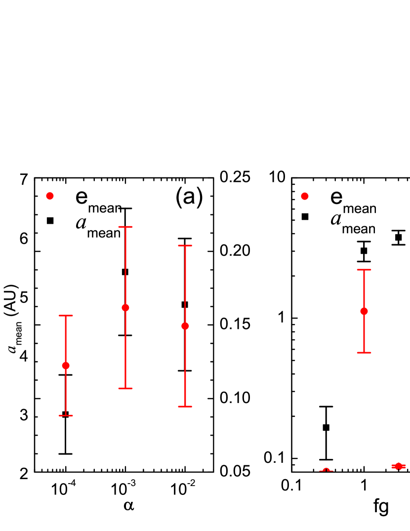
Figure 3: The influences of survival system properties due to different gas disks. The left vertical axis presents mean semimajor axis while the right one presents mean eccentricity. (a) influence of effective viscosity parameter $\alpha$, (b) influence of the disk mass. the error bars are the standard deviations.

In our model $\alpha_{\rm dead}$ mainly works on type I migration via Eq.(9) and type II migration via Eq.(16). Since $\Sigma_{g}\propto(\alpha_{eff})^{-1}$ (Eq.[6]), thus $\tau_{\rm mig,I}\propto\alpha_{eff}$, i.e., planets in disks with smaller $\alpha_{eff}(\sim 10^{-4})$ migrate faster, which results in a smaller average semimajor axis(Fig.3a). For type II migration, if the planet mass is small ($M_{p}\leq 2\Sigma_{g}a^{2}$, which is about $90M_{\oplus}$ at 5AU and $170M_{\oplus}$ at 10AU), the migration speed decreases with $\alpha_{eff}$, thus larger $\alpha_{eff}$ ($\sim 10^{-2}$) may also lead to a small average semimajor axis. Thus the disk viscosity may change the final location of the planets. So we take a most plausible value ($\alpha_{\rm dead}=10^{-4}$) in the following simulations(Sano et al. 2000). On the other hand, the average eccentricities are around 0.1 with large variations for all cases, which seems to be insensitive with $\alpha_{\rm dead}$. The reason is that small $\alpha_{\rm dead}$ leads to a high density of gas disk, resulting in two competing effects: (a) a fast type I migrations so that a large frequency of embryo-scatterings is expected, which enhance the eccentricities of embryos. (b) a fast $e$-damping rate with a small $e_{\rm mean}$. As the timescales of these two effects are comparable, $e_{\rm mean}$ is nearly independent of $\alpha_{\rm dead}$.

There are three ways for $f_{g}$ to influence the orbital evolutions: the surface density of the gas disk(Eq.[6]) , initial isolation masses (Eq.[7] with $f_{d}=f_{g}$), and the critical mass for the onset of runaway gas accretion (Eq.[11]). Larger $f_{g}$ may result in larger cores extended to an outer region. As we assume $\dot{M}_{\rm core}\propto f_{d}$, we have $M_{\rm crit}\propto f_{g}^{0.25}$. Comparing with the masses of the initial embryos($\propto f_{g}^{3/2}$), it’s much easier to form massive gas giants in a massive gas disk.

As shown in Fig.3b, when $f_{g}\geq 1$, $a_{\rm mean}$ are all around $3-4$AU. Although the migrations should be faster for planets in disks with larger $f_{g}$, the initial embryos extended to an outer region in these cases, which results in similar averaged locations. For a less massive disk($f_{g}=0.3$), these small embryos initially in the inner region have never accreted gas, and thus they experienced type I migration throughout the evolution, therefore they have smaller $a_{\rm mean}$ and $e_{\rm mean}$. More effective eccentricity-dampping results in a smaller $e_{\rm mean}$ for $f_{g}=3$ than that of $f_{g}=1$. When $f_{g}=10$, the largest embryos can reach $~{}80M_{\oplus}$ via collisions in 1Myr. Finally the planets left in these systems are mainly gas giants, and their eccentricities are damped much less effectively than those of small planets. This is why $e_{\rm mean}$ of $f_{g}=10$ is much larger than that of $f_{g}=3$.

4.2 Correlations with the disk lifetime ( $\tau_{\rm disk}$)

The role of the gas disk on the planet evolution is manifold: it causes the inward migration (type I or II) of protoplanets as well as the tidal damping of their orbital eccentricities. A long survival gas disk may be helpful to the formation of giant planets, while planets in a short-lived disk may not have enough time to accrete gas, thus remain either terrestrial or Neptunian planets. To investigate the effect of the disk depletion timescales ($\tau_{\rm disk}$), we set 11 values of $\tau_{\rm disk}$, evenly ranged from 0.5 Myr to 5Myr in a logarithm scale (Haisch et al. 2001). For each $\tau_{\rm disk}$ we did 20 runs of simulations by choosing the orbital phase angles of the embryos randomly. So totally we did 220 simulations for $f_{g}=1$. All the simulations are stopped at $t=10$ Myr.

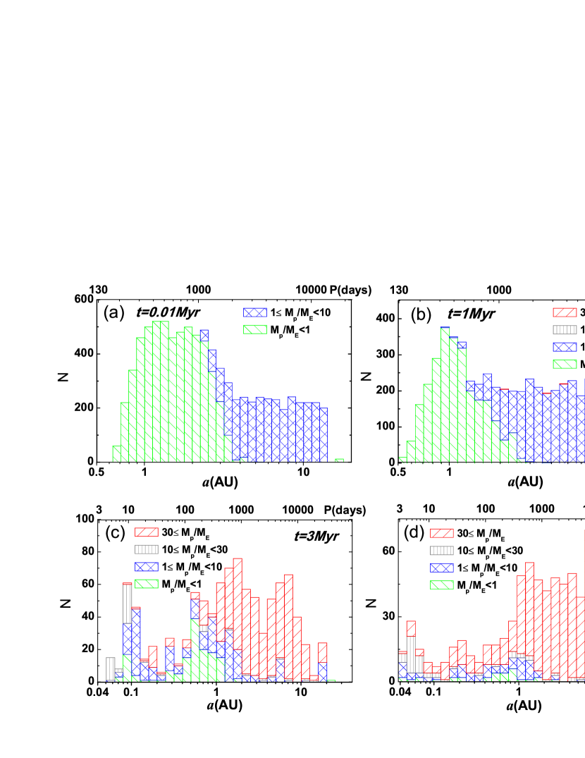
Figure 4: Distributions of semimajor axes for the survival planets in the 220 runs of simulations at different epoches: (a) 0.01 Myr, (b) 1Myr, (c) 3 Myr, (d) 10Myr during the evolution.

An interesting problem for planet formation is the growth epoch of different types of planets. We define (somewhat arbitrary) the following two types of planets: gas giant planets (GPs), includes massive GPs ($M_{p}\geq 30M_{\oplus}$) and Neptune-sized GPs ($10M_{\oplus}\leq M_{p}<30M_{\oplus}$); terrestrial planets (TPs), including Super-Earth TPs ($1M_{\oplus}\leq M_{p}<10M_{\oplus}$) and Sub-Earth TPs($M_{p}<1M_{\oplus}$). Fig.4 shows the distribution of planet semimajor axes for the 220 runs of simulations at some epoches with $f_{g}=1$. Only TPs are present at $t=10^{4}$yr (Fig.4a). When $t=1$Myr, runway gas accretion occurred, thus a few GPs appear (Fig.4b). The most efficient growth of GPs occurred at $1-3$Myr, thus the number of GPs increased very fast (Fig.4c), until they become the dominant members at the end of simulations(Fig.4d).

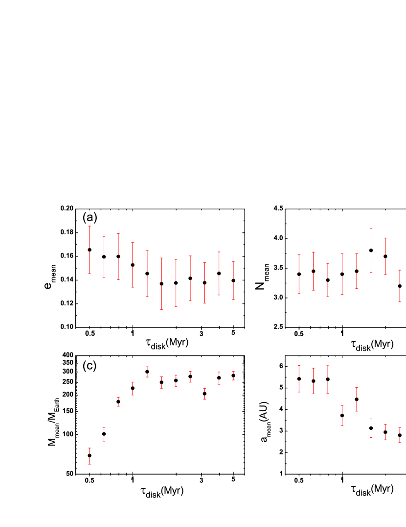
Figure 5: Correlations between the parameters of survival systems and the disk depletion timescale ($\tau_{\rm disk}$) in 220 runs of simulations. Each point is average over 20 runs of systems with same $\tau_{\rm disk}$, with error bars indicating the standard deviation. Panels from (a) to (d) shows the average eccentricities, numbers, masses and semimajor axes of the surviving planets versus $\tau_{\rm disk}$.

Fig.5 plots the correlations between the properties of the final systems and $\tau_{\rm disk}$. Basically there are two regimes. For short-lived disks with $\tau_{disk}\leq 1$Myr, the forming planets have small average masses ($70-200~{}M_{\oplus}$, Fig.5c), the average semimjor axes of these systems are large ($5-6$AU, Fig.5d), indicating most of the surviving planets were formed in distant orbits, while migrations have not affected their orbital architectures strongly. The average eccentricities ($\sim 0.15$) are relatively big (Fig.5a), showing the tidal damping effect is not very effective due to the short lifetime of the disk. On the contrary, planetary systems with a longer disk lifetime ($\tau_{disk}>1$Myr) tend to have larger average planet masses ($\sim 1$ Jupiter mass ), with lower averaged eccentricities ($\sim 0.1$) due to the long period of the disk damping. The semimajor axes of these systems decrease from 4 AU to 2 AU, indicating inward migration indeed plays an important role in sculpting their orbital configurations.

Systems with $\tau_{\rm disk}<1.5$Myr do not have much differences on the surviving number of the planetary systems, while $N_{\rm mean}$ decrease slightly as $\tau_{\rm disk}>1.5$Myr increasing (Fig.5b). The maximum of $N_{\rm mean}$ at $\sim 1.5$Myr, is due to the mechanism of halting small planets near $a_{\rm crit}$ (see §5.1). In disks with smaller $\tau_{\rm disk}$, the effects due to gas disks are not so efficient, and the surviving number of planet systems mainly depends on the interactions between embryos. In the disks with longer lifetime, giant planets experience sufficient type II migration and will be closer to the boundary of MRI region, where small planets were halted (see §5.1). Thus small planets are easier to be scattered out of the system or hit the host star, leaving fewer surviving planets.

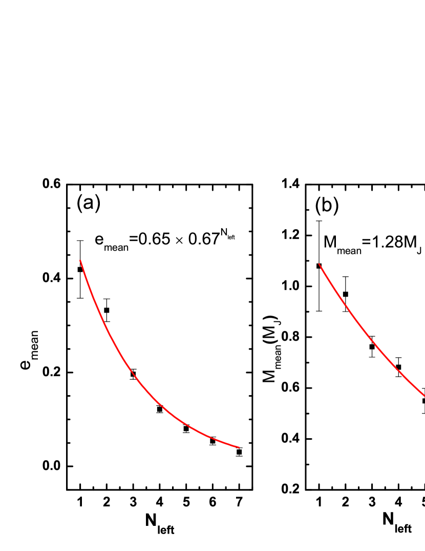
Figure 6: The correlations between the survival planet number $N_{\rm left}$ and the averaged eccentricity $e_{\rm mean}$ (a) as well as the average planet mass $M_{\rm mean}$ (b) in a planetary system. Both $e_{\rm mean}$ and $M_{\rm mean}$ are inversely correlated with $N_{\rm left}$. The error bars are the standard deviations.

One of the major effects that N-body simulations can describe is the eccentricity excitation due to mutual planetary perturbations. Such excitation may lead to some embryos being scattered out of the system, while others may be merged. Thus the final number of the planets should be greatly reduced from that of the initial embryos. Correlations between the number of survival planets and the averaged mass as well as eccentricity of the planets in a planetary system are shown in Fig.6. They are fitted by

$$e_{\rm mean} = 0.65\times 0.67^{N_{\rm left}},$$

$$M_{\rm mean} = 1.28M_{J}\times 0.85^{N_{\rm left}}.$$ (24)

These correlations show that, in multi-planet systems like solar system, planets basically have relative lower averaged masses and eccentricities than those with single or few planets. Qualitatively, this law is easy to be understood. In order to achieve a longer orbital crossing time in a multi-planet system, either the eccentricities of the planets must be small, or the planets should have large mutual separation scaled by their Hill radii, thus smaller planetary masses is helpful to achieve a stable system(Zhou et al. 2007).

5 Comparing with Observations

To compare our results with the observations, we set the mass of the disk ($f_{g}$) and its depletion timescale ($\tau_{\rm disk}$) as two free parameters. We take 11 values of $\tau_{\rm disk}$ evenly ranged from 0.5 Myr to 5Myr in a logarithm scale(Haisch et al. 2001). For each $\tau_{\rm disk}$, we choose $f_{g}=0.3,1,3,10$, and execute 6,10,5,3 simulations, respectively, to fit for the Gaussian distribution of $\log{(M_{disk}/M_{\odot})}$ with a mean value of $\mu=-1.66$ and a standard deviation $\sigma=0.74$, according to the observations of Taurus-Auriga (Mordasini et al. 2009a). So totally we execute $11\times 24=264$ runs of simulations.

We also make some statistical plots from the observed systems. To show planets that may be not observable yet, we distinguish planets of our simulations with detectables (with the induced stellar radial velocity $V_{r}\geq 3~{}$m s^-1) and undetectables ($V_{r}<3~{}$m s^-1). Taking the mean value of $\sin i=0.6$, among the 1437 survival planets, 959 planets ($66.7\%$ of total ) from our simulations are undetectable, which contains a large number of small planets ($<1M_{\oplus}$).

5.1 Semimajor Axis Distributions

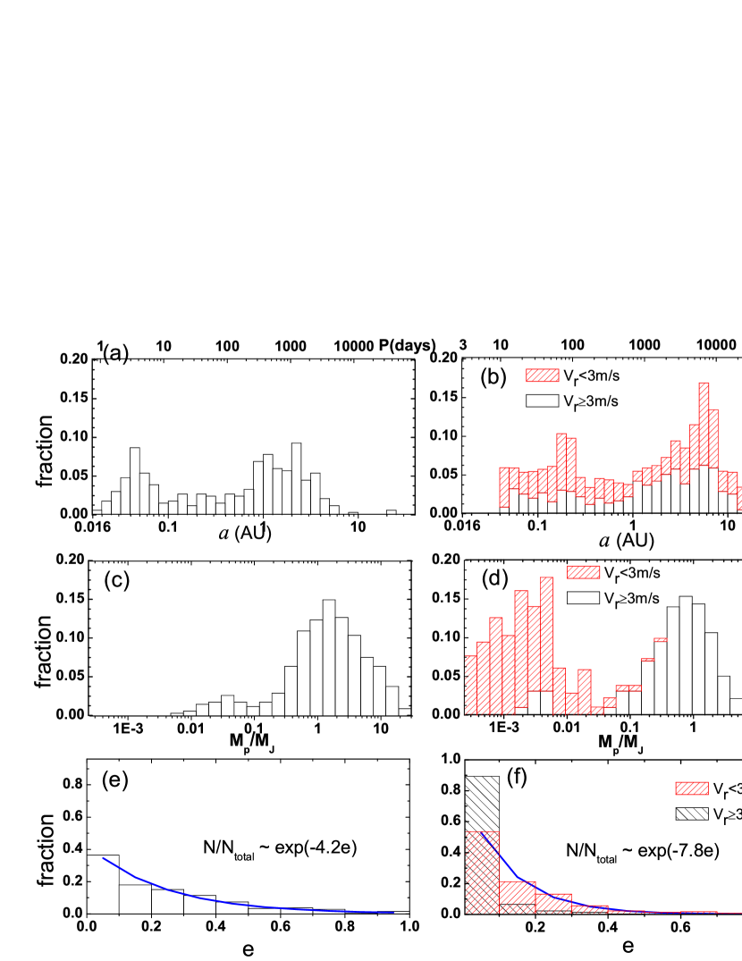
Figure 7: Distributions of semimajor axes, eccentricities and planet masses ($a,e,M_{p}$, resp.) from observations (left column, data: http://exoplanet.eu) and our simulations (right column). The shaded bars in (b),(d),(f) show distributions of the undetectable planets (with radial velocity $V_{r}<3{\rm m/s}$). The solid curves in (e) and (f) are fitting curves by $N(e)/N_{\rm total}=0.1A\exp(-Ae)/[1-\exp(-A)]$, with $A=4.2$ for observations (e) and $A=7.8$ for simulations of planets with $V_{r}>3{\rm m/s}$ (f).

Fig.7a and b show the semimajor axis distribution from both the observations and the simulations. The observed distribution shows two peaks(Fig.7a). (1) At 1-3AU. This is roughly the snow line (where water is frozen) of the system, where planet cores may be stalled under type I migration (Kretke & Lin 2007, Ida & Lin 2008), subsequent accretion of gas makes them giant planets. (2) At 0.04-0.06AU (or 3-5 days). This is roughly the inner edge of the gas disk, where planets under type II migration will be stopped (Lin et al. 1996). From our simulations there are lots of planets beyond 3AU, thus the lack of planets at $>3$ AU is due to observational bias.

Besides, we show that there is an extra pile-up of planets: (3) at around 0.2AU (or around 30 days), which has not been revealed by observation yet. This location corresponds to the inner edge of the MRI dead zone ($a_{\rm crit}$) where small planets under type I migration may be halted. However, as the location of $a_{\rm crit}$ (See Eq.[8]) moves inward, in the case of short $\tau_{\rm disk}$, its migration speed is faster than that of the type I migration, therefore it is difficult to halt these planets near $a_{\rm crit}$. When $\tau_{\rm disk}\sim~{}1.5$Myr, $\frac{da}{dt}\mid_{\rm mig,I}\sim\frac{da_{\rm crit}}{dt}$, so if $\tau_{\rm disk}>1.5$ Myr, the mechanism of halting small planets near $a_{\rm crit}$ works. After $\tau_{\rm disk}$, the migration rate is reduced due to gas depletion. In fact, $a_{\rm crit}\sim 0.2$ AU at $t=2\tau_{\rm disk}$. This explains the accumulation of planets near $0.2$AU. Some small planets were scattered into $0.04$AU.

Our simulations also show that, the majority ($70\%$) of giant planets is located in $1-10AU$. Most of them are massive GPs and experienced type II migration. Due to the depletion of the gas disk, they can not migrate to the proximity of the star, hence they halted outside $1$ AU. Due to observational bias of radial velocity measurements, only those massive giant planets at $<4-5$AU are revealed.

5.2 Mass Distributions

Our simulations show mainly there are two peaks for planet masses: (Fig.7c).

(1) At 1-2$M_{J}$. They are Jupiter-sized giant planets that have grown up with efficient gas accretion. Although our simulations reproduced this peak, there are not enough amount of massive planets at $M_{p}\sim 5-8M_{J}$.

(2) At $0.1-3M_{\oplus}$. There are a large number of terrestrial planets, which have grown up mainly by mutual collisions under the perturbations of outside giant planets. This peak has not been revealed by the observations yet, and can be checked by future observations of terrestrial planets.

One more small peaks are revealed by our simulations:

(3) Around $10M_{J}$. Massive embryos ($M\sim 80M_{\oplus}$) had been formed after 1Myr in disks with $f_{g}=10$ and only experienced time-limited type II migration. More massive giant planets($>10M_{J}$) may be born with some other mechanisms, e.g., the gravitational instability scenario.

The desert at $10-20M_{\oplus}$ are Neptune-sized planets. According to our model in Section 2.3, the Kelvin-Helmholtz timescale are quite short($\sim 10^{4}$yr) for this mass regime and the runaway gas accretion makes them become giants quickly. Only a few planets in the inner region with $M_{\rm iso}\sim 10-20M_{\oplus}$ survive in this desert. Also merging from lower planet embryos is possible to form Neptune-sized planets.

5.3 Eccentricity Distributions

The distribution of eccentricities from simulations is similar to that from observations. In our simulations, the eccentricities of survival planets vary from $0$ to $0.84$, while the observations show a maximum eccentricity of about $0.9$ (Wright et al. 2009). We fit both distributions (simulations and observations) with an exponential decay function in the form of $P(e)de=N(e)/N_{\rm tot}\sim\exp(-Ae)de$. Since $\int^{1}_{0}P(e)de=1$, we have

$$P(e)=\frac{A\exp(-Ae)}{1-\exp(-A)}.$$ (25)

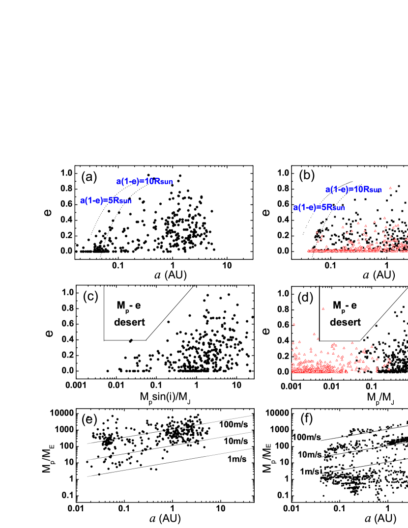
Figure 8: Correlation graphes from observations(left column, data: http://exoplanet.eu) and our simulations (right column). Planets with induced stellar radial velocities $V_{r}<3{\rm m/s}$ are shown in red triangles. Solid lines in (e) and (f) show the induced stellar radial velocities. The boxes in (c) & (d) show the planet desert in the $M_{p}-e$ diagram.

where $A=4.2$ for observations and $A=7.8$ for simulations of planets with $V_{r}<3m/s$, as shown in Fig.7e and Fig.7f. The larger value of $A$ from simulations indicates a steeper slope, showing more planets with small eccentricities are still not detected, as shown in Fig.8d later.

5.4 Correlation Graphes between $a,e$ and $M_{p}$

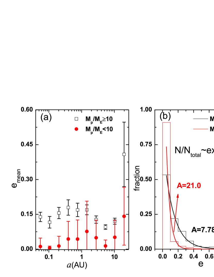
Figure 9: Variations of mean eccentricities with semimajor axes (a) and distributions of eccentricities (b) for giant planets ($M_{p}\geq 10M_{\oplus}$) and terrestrial planets ($M_{p}<10M_{\oplus}$). Histograms in (b) are fitted by $N(e)/N_{\rm total}=0.1A\exp(-Ae)/[1-\exp(-A)]$, with $A=7.78$ for giant planets and $A=21.0$ for terrestrial planets.

Figure 8 presents the correlation diagrams of $a,e$ and $M_{p}$ of our simulations (right), with a comparison to the observational data (left). Our simulations reproduced all the three correlation plots quite well. Especially there is a gap in the $M_{p}-e$ plot, indicating a planet desert ($0.005\sim 0.08M_{J}$) depends on the eccentricity (Fig.8c & d). Fig.8d also shows a tendency that giant planets ($M_{p}>10M_{\oplus}$) tend to have lager eccentricity on average. To show this more clearly, we reproduce the eccentricity-semimajor axis correlation plots and the eccentricity distribution plots for giant planets ($M_{p}>10M_{\oplus}$) and terrestrial planets ($M_{p}<10M_{\oplus}$) in Fig.9. Giant planets have average eccentricities $\sim 0.15$ at all locations (except $>10$AU), while terrestrial planets have average eccentricities $\sim 0.05$. Although both of the e-distribution can be fitted by exponential law in Eq.(25), their coefficients A are different : 7.78 for $M_{p}>10M_{\oplus}$ and 21.0 for $M_{p}<10M_{\oplus}$, indicating small mass planets tend to have smaller eccentricities.

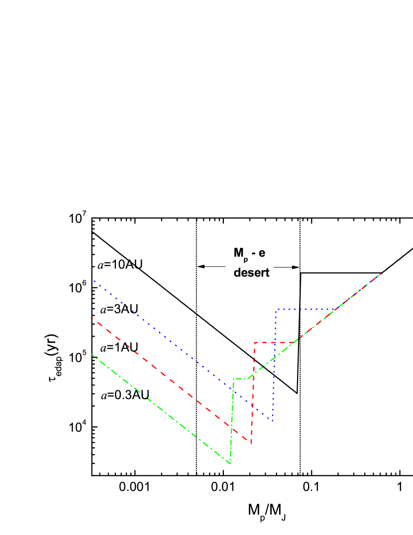
Figure 10: Variations of eccentricity damping timescale ($\tau_{edap}$) for different planet masses ($M_{p}$) at semimajor axes 0.3AU, 1AU, 3AU and 10 AU. For those planets $M_{p}<M_{I,II}$, $\tau_{edap}$ is calculated by Eq.(10) using a mean eccentricity $e=0.05$. Otherwise $\tau_{edap}$ is calculated by Eq.(17). The jump of $\tau_{edap}$ occurs at $M_{p}=M_{I,II}$. $\tau_{edap}$ keep horizontal until the mass of the planet becomes comparable to the disk mass. The $M_{p}-e$ desert in Fig. 8d roughly corresponds to the mass regime with $\tau_{edap}$ less than $\sim 1Myr$. Out of this region eccentricities of planets can hardly be damped.

To understand the $M_{p}-e$ desert, i.e., very few planets with masses $0.005\sim 0.08M_{J}$ have eccentricities larger than $0.3-0.4$, we plot the $e$-damping timescales $\tau_{edap}$ as a function of planet masses at 0.3, 1, 3 and 10AU in Fig.10. For a planet, when $M_{p}<M_{I,II}$, $\tau_{edap}$ is calculated by Eq. (10) using a mean eccentricity $e=0.05$ and $\Sigma_{0}=280$ g cm^-2. Otherwise $\tau_{edap}$ is calculated by Eq. (17) with viscosity $\alpha_{\rm dead}=10^{-4}$. Due to Eq. (10), small planets have longer $\tau_{edap}$. The jumps of $\tau_{edap}$ occur at $M_{p}=M_{I,II}$. $\tau_{edap}$ keeps horizontal until the mass of the planets becomes comparable to the disk mass ($M_{p}>2\Sigma_{p}a_{p}^{2}=21M_{\oplus}(a/1\rm AU$)). In the braking phase of type II migration, more massive planet have a longer $e$-damping timescale according to Eq. (17). Assuming an effective damping of eccentricity if $\tau_{edap}$ is less than $\sim$ 1Myr, we obtain a mass regime $0.005\sim 0.08M_{J}$ which is consist with the $M_{p}-e$ desert from both observations and our simulations in Fig.8c & d. As shown in Fig.10, $\tau_{edap}$ of massive GPs is in the horizontal region or beyond this, so generally they have longer $e$-damping timescales than those of the TPs. Therefore, the mean eccentricity of TPs is smaller than that of GPs.

6 Simulations in Three-Dimensional Model

In all the above simulations, we adopted coplanar planetary model (2D). When the orbital inclinations of the planets (3D) are included in the simulations, their final orbital characteristics of the planet systems may be changed due to the different collision timescales between 2D and 3D simulations (Chamber, 2001). In this section, we reveal the effects of including orbital inclinations with some more simulations. We executed 20 runs in 3D model, setting the same initial conditions with those in 2D model except that the initial inclinations are set as 1 degree for all embryos, with randomly chosen. The disk parameters are also set as a standard value in our simulations: $f_{g}=1,\tau_{\rm disk}=2$Myrs and $\alpha_{\rm dead}=10^{-4}$.

6.1 Collisions with Different Masses

During the whole evolution period we simulated (10Myrs), there are 606 collisions in the 20 runs of 2D simulations, while 471 collisions occurred in the corresponding runs of 3D model. In the 2D runs, the number of embryos colliding with the host star or being ejected out of the system is 120, comparing with the number of 231 in 3D runs. It is consistent with the result of Chambers (2001). As seen in Fig.11a, the cumulative distribution functions (CDF) of collisions in two models show that most collisions in 3D runs occurred in relatively later stages. Thus earlier collisions in 2D model produce embryos with larger masses. To show the effects of earlier collisions to the final planetary architectures, we divided the collisions as three regions, as shown in Fig.11b: Region I ($M_{0}<M_{\rm crit},M_{1}<M_{\rm crit}$), II ($M_{0}<M_{\rm crit},M_{1}>M_{\rm crit}$) and III ($M_{0}>M_{\rm crit},M_{1}>M_{\rm crit}$), where $M_{0}$ represents the larger mass of the embryo before a two-body collision, while $M_{1}$ represents that after the collision, $M_{\rm crit}=4M_{\oplus}$ is the critical mass beyond which the efficient gas accretion sets in (see discussions below Eq.[11] ).

Region I: Most collisions (2D: $\sim 75\%$, 3D: $\sim 85\%$) occurred in this region. These collisions only influence the Earth-like planets(TPs, see §4.2). Due to the shorter collision timescale in 2D model, embryos have larger masses on average during early time and experience faster type I migrations and $e$-damping according to Eq[9] and Eq[10]. Therefore the TPs have a smaller mean eccentricity (c.f., $e_{\rm mean}=0.034$ for 2D and $e_{\rm mean}=0.047$ for 3D) and semimajor axis (see Fig.11c). As a results of more collisions occurred in 2D simulations, the final systems are expected to have less number and larger masses of TPs than those from 3D simulation. In fact, we find 11 TPs left among the total 74 survived planets in the 20 runs of 2D simulations, while it is 24 out of the total 98 survivals in the corresponding 3D simulations, with a small average mass (Fig.11c).

Region II: About $8.5\%$ (2D) and $8.4\%$ (3D) collisions occurred in this region. These collisions makes the embryos with masses $<M_{\rm crit}$ grow beyond the critical mass. However, this effect is limited by the small fraction of collisions and the slow gas accretion rate(Eq[12]) for embryos with masses slightly larger than $M_{\rm crit}=4M_{\oplus}$. Thus the differences between 2D and 3D models due to collisions in this region can be ignored.

Region III: Roughly $\sim 16.5\%$ (2D) and $\sim 6.6\%$ (3D) collisions occurred in this region. These embryos can accrete gas before collisions. As type I migrations speed is much faster than that of type II, the final locations of the planets are mainly determined by their planets cores. As planet cores in 2D model undergo more collisions, they have bigger masses thus a fast migration speed, so their final average semimajpr axis is small than that in 3D (Fig.11d). As inner region has less gas to accretion, $M_{\rm gas}\propto\Sigma_{g}aR_{H}$, while $R_{H}\propto(M_{p}/3M_{*})^{1/3}a$ and $\Sigma\propto a^{-1}$), the final giant planets in 2D simulations have less masses(Fig.11d). As the type I eccentricity damping rate is much small than that of type II (Fig.10), and from Eq.(10), $\tau_{\rm edap,I}\sim a^{1/2}M_{p}^{-1}$, thus larger masses of planets in 3D simulations have shorter $\tau_{\rm edap,I}$, thus the mean eccentricity ($e_{\rm mean}\approx 0.086$ by simulations) in 3D model is smaller than that ($e_{\rm mean}\approx 0.15$) in the 2D model.

6.2 Differences in Statistics

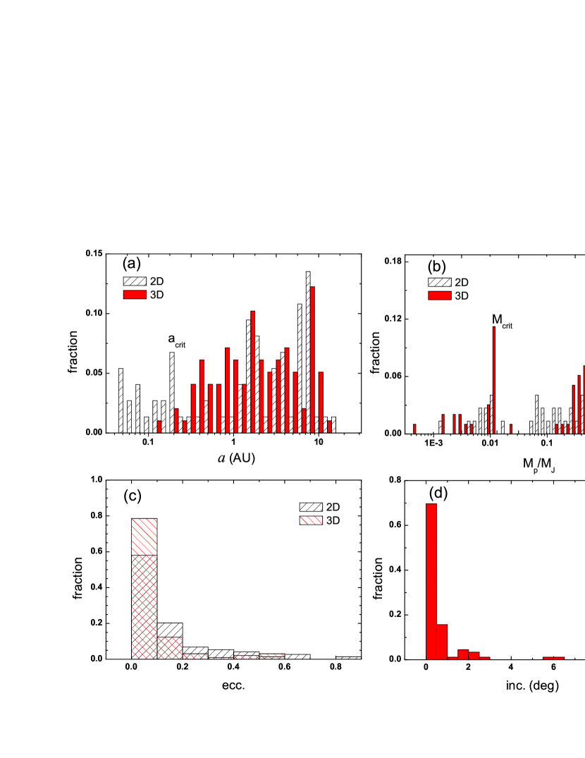
Figure 12: Distributions of (a) semimajor axis, (b) planetary masses, (c) eccentricities and (d) inclinations of the survival planets in 20 runs of 2D simulations and 20 runs of 3D simulations, respectively.

As most of our results in §5 are in statistics, we focus on the statistical differences between 2D and 3D two models. The statistics of semimajor axes and masses of planets in two models are presented in Fig.12. Some peaks and deserts in 2D model are reproduced in 3D model, such as the peaks at $a_{\rm crit}\sim 2$AU, $M_{\rm crit}$ and $1-2M_{J}$. However, There are still some different characteristics, especially the planet deserts at around $0.1$AU and $10M_{\oplus}<M_{p}<0.1M_{J}$ in 3D model. The lack of planets around $0.1$ AU in 3 D model may be due to the prolonged collision timescale, a much longer time of integration may results similar qualitative results with 2D model. The deficit of planets with masses $10M_{\oplus}<M_{p}<0.1M_{J}$ in 3D model make the planet desert in §5.2 more obvious.

Fig.13 shows the orbital inclination distribution for the survival planets in the 20 runs of 3D simulations. As one can see, most of the planets remain in $<2$ degrees, only few planets with smaller masses have inclinations $\sim 10$ degrees.

To summary, we point out that the differences between 2D and 3D simulations are not much, most of statistical results in 2D are qualitatively credible.

7 Conclusions and Discussions

Based on the standard core accretion model of planet formation, we simulated the final assemble of planets by integrating the full N-body equations of motions. The stellar mass is fixed at $1M_{\odot}$. The circumstellar disk is assumed to have an effective viscosity parameter $\alpha_{\rm eff}$ (Eq.[4]), and undergoes an exponential decay in a timescale of $\tau_{\rm disk}=0.5-5$Myr. Initially embryos with isolation masses larger than $0.1M_{\oplus}$ (Eq.[7]) are put in each system. For embryos below (or above) the critical mass defined in Eq. (14), they will undergo type I (or type II, resp.) migration. The type I migration of embryos will be stalled near the inner edge of the MRI dead zone defined in Eq.(5). The inner edge of the disk is set as $0.05$AU where giant planets will be stalled under type II migration. The equations governing the embryo’s motions are shown in Eq. (19).

We have investigated the influences of different parameters(viscosities, disk masses, disk depleted timescales) on the final architectures of the planetary systems. Disk viscosity affects the planet locations by determining their migration speeds. In the regime of $\alpha_{\rm dead}\in[10^{-4},10^{-2}]$ , planets in disks with small viscosities migrate fast under type I planet-disk interactions, which results in a small average semimajor axis. For a moderate disk viscosity, the planetary system shows a moderate averaged locations (Fig.3a). The average eccentricity does not show obvious correlation with the disk viscosity. Disk mass affects the system through the initial core masses. Large planet cores can be formed in the outer region of a massive disk, so that giant planets are easier to form.

Disk depletion timescale ($\tau_{\rm disk}$) plays an important role in final planetary masses and orbits. For short-lived disks with $\tau_{\rm disk}\leq 1$Myr, the forming planets have small masses ($70-200~{}M_{\oplus}$), with large average semimjor axes ($5-6$AU). This indicates that most of the surviving planets are formed in distant orbits, while planet migrations did not affect their orbital architectures yet. Due to the short lifetime of the disk, their average eccentricities ($\sim 0.15$) are relatively big. Planetary systems with a long-lived disk ($\tau_{\rm disk}>1$Myrs) tend to have large planetary masses ($\sim 1$ Jupiter mass ), with low averaged eccentricities ($\sim 0.1$) due to the long time disk-damping. The average semimajor axes of these planets are ranging from 4 AU to 2 AU, indicating inward migration indeed plays an important role in making planets in close-in orbits.

Comparing the simulations to others, we find the number of planets being trapped in mean motion resonances (MMRs) are smaller than those obtained, such as in Terquem & Papaloizou (2007). Instead, we get a large amount of planet pairs that have the history of passing periastron alignment (See Table 2, with the difference of their longitude periastron librating at $0^{o}$). The reason that we did not observe many survival planets in MMRs may be due to the fact that, most of our survival planets are giant planets. The choice of a small disk viscosity ($\alpha_{\rm dead}=10^{-4}$) makes the type II migration too slow to make a significant convergent MMR trapping. For terrestrial planets, the speed of type I migration is faster than that of type II migration of the giant planets in outside orbits, so they are not easy to be trapped into the MMRs of giant planets as well.

Statistics of 264 simulated systems reproduced qualitatively the main features on the planet masses and orbital parameters for the observed exoplanetary systems. If we classify the planets into two major categories: giant planets (GPs), including massive GPs ($M_{p}\geq 30M_{\oplus}$) and Neptune-sized GPs ($10M_{\oplus}\leq M_{p}<30M_{\oplus}$); terrestrial planets (TPs), including Super-Earth TPs ($1M_{\oplus}\leq M_{p}<10M_{\oplus}$) and Sub-Earth TPs($M_{p}<1M_{\oplus}$), then results from our simulations have the following implications on these planets.

Occurrence rates of planets. The ratio of GPs relative to TPs is low, i.e., 514 to 923 (or 36% to 64%) in our total 1437 survival planets (table II). This is mainly due to the fact that only those massive embryos can accrete sufficient gas to form GPs. Planets with smaller masses are easier to be scattered out by N-body interactions, which is the major difference with the population synthesis simulations of single-planet systems. Moreover, there exist some correlations between the survival number of planets and the average eccentricity (or average planet mass) of a planetary system, i.e., a planetary system with more planets tends to have smaller planet masses and orbital eccentricities(Fig.6 and Eq. [24]). These correlations are consistent with the stability of the system, i.e., a system with planets in less eccentric orbits and with larger mutual separation scalled by their Hill radii tends to have longer crossing timescale, thus is more stable (Yoshinaga et al. 1999, Zhou et al. 2007).

Locations of giant planets (GPs). Most (298, $\sim 58\%$ of total 514 ) of GPs locate at orbits with semimajor axes 1-10 AU , with only $\sim 35\%$ (182) at inner orbits $<1$ AU. This may be linked with the snow line ($\sim 2-3$AU) of the system. Due to the surface density enhancement of about $3-4$ (Eq. [7]), isolated masses beyond the snow line are larger thus they are easier to accrete gas and become giant planets. Neptune-sized GPs are formed in our simulations also, with its amount being much smaller than massive GPs ( $\sim 7.5\%$, 42 of 1437), and they mainly locate at two parts of the systems: either at $\sim 10$AU, which were scattered out by first formed giant planets (like the formation of Uranus and Neptune), or in the inner edge of the gas disk ($0.05$AU), which seems to be stalled there under type II migration.

Locations of terrestrial planets (TPs). TPs are almost evenly distributed, except a group lying at 1-2 AU(Fig.4d, for $f_{g}=1$), just inside the snow line($\sim 3$AU). Also there is a slight pileup of planets (both GPs and TPs) at $0.2-0.3$AU (30-50days), which may correspond to the inner boundary of the MRI dead zone. According to Kretke & Lin (2007) and Morbidelli et al. (2008), super-Earths are easier to be stalled there from type I migration, and grow up to giant planets by gas accretion.

Eccentricities of planets. There are very few planets with masses $0.005\sim 0.08M_{J}$ that have eccentricities larger than $0.3-0.4$, The average eccentricities of giant planets are larger ($\sim 0.15$) than those of the terrestrial planets($\sim 0.05$, Fig.9). According to our simulations, the underlying mechanism is the relatively long $e$-damping timescale of massive planets due to the gas disk, especially when the planet mass is larger than the inner disk mass, see Eq.(16) and Eq.(17).

We compared our results with some 3D simulations in §6. The qualitative differences between 2D and 3D models are not big, indicating our conclusions based mainly on 2D simulations are still reliable.

Now let’s compare above conclusions to the five new observational signatures that stated in §1. According to our simulations, 260 runs in total 264 ones result in multi-planet systems, which rates to $98\%$, comparing with that from the observations ($>28\%$). Planets in multiple systems have smaller eccentricities than single planets, which is revealed clearly in Fig.6. For signature-2, we did not classify our $a,e$ and $M_{p}$ distributions with single and multiple systems, as this classification has some uncertainty concerning undetected planets. While Fig.9a supports signature-3, massive planets seem to have larger eccentricities than those of smaller mass planets. The implication of this is interesting. As most of the observed exoplanets have Jupiter-sized planets in elliptical orbits, we can expect more planets with small masses in near circular orbits of multi-planet system, like terrestrial planets in the solar system. Signature-4, i.e., massive planets tend to have larger eccentricities, is revealed by our simulations (Fig.9b). For signature-5, as we fix the stellar mass at $1~{}M_{\odot}$, it can not be tested in the present work. We will investigate this correlation in future works.

However, due to some limits and uncertainties of the parameters we chose in this model, the conclusions obtained in the paper may be limited. For example, we investigated planet formation around 1 $M_{\odot}$ stars only, although with different sizes of the solid and gas disks. Not only the disk mass but also the accretion rate as well as metallicity have correlation with the mass of the host star. For more broader parameters, the occurrence ratio of planets between TPs and GPs may need further investigations.

One of the major uncertainties arises from the initial masses and distributions of the embryos, which are the building blocks of planets. In this paper, we adopt the assumption that most of the embryos have already cleared their nearby heavy elements and achieved their isolation masses. This assumption is based on the full N-body simulation of planet growth (Kokubo & Ida 1998), and will be too ideal when type I migration of embryos are taking into considerations. Also, initially there might be some smaller embryos between giant planets so that they may be scattered through planet scattering and become planets like Uranus and Neptune.

The second major uncertainty comes from our poor knowledge of type I migration of the embryos. The speed (and even the direction) of type I migration will affect the number and locations of survival terrestrial planets, especially planets in habitable zones (e.g., Ogihara & Ida 2009, Wang & Zhou 2010). We will do more investigations to that end in our forthcoming works.

Thirdly, our simulations mainly focus on the stage that the gas disk is present and will be depleted exponentially. Further evolution due to the effect of a planetesimal disk was not included. During the later stage of planet formation when the gas disk is totally depleted, planet-planetesimal interactions may damp the eccentricities of planets through dynamical frictions, and may induce migrations through angular momentum exchanges with embryos and scattered planetesimals (Fernandez & Ip 1984; Malhotra 1993). In the solar system, numerical simulations show that, Jupiter will drift inward, while Saturn, Uranus and Neptune may migrate outward, resulting in a divergent migration. During the migration, the cross of 2:1 MMR between Jupiter and Saturn excites the eccentricities of four giant planets (Tsiganis et al. 2005). Such evolution may occur on the timescale of at least hundreds of million years, which is beyond the ability of our simulations.

Furthermore, we ignored the tidal effect between a host star and close-in planets. The tidal dissipation of the star-planet system may damp the eccentricity of the planets in close-in orbits in a Gyr timescale. Also, the gravitational potential of the gas disk was not included in our model. During disk depletion, the sweeping of secular resonance through inner region may excite the eccentricities of inner orbits, thus induce further mergings of terrestrial planets (Nagasawa et al. 2003).

Although with many restrictions, the present paper, aiming at the statistics of final assembling of planetary systems in the standard formalism (which includes type I and type II migration, gas accretion, etc.), reproduces most of the observed orbit signatures. Thus we think that the predictions by the simulations are helpful for guiding future planet detections.

Acknowledgements Zhou is very grateful for the hospitality of Issac Newton institute during the program of ’Dynamics of Discs and Planets’. This work is supported by NSFC (10925313,10833001, 10778603), National Basic Research Program of China (2007CB814800), and a Fund from the Ministry of Education, China (20090091110002).

Table 1: Notations used in the paper, $\tilde{M}_{*}=M_{*}/M_{\odot},\tilde{r}=r/1{\rm AU}$,

. $T=280\tilde{M}_{*}\tilde{r}^{-1/2}$ disk temperature by stellar radiation $c_{s}=1.2{\rm km~{}s}^{-1}\tilde{M}_{*}^{1/4}\tilde{r}^{-1/4}$ sound speed in the ideal gas with adiabatic index $\gamma=1.4$ $v_{k}=29.8{\rm km~{}s}^{-1}\tilde{M}_{*}^{1/2}\tilde{r}^{-1/2}$ orbital speed of Kepler motion $h=rc_{s}/v_{k}=0.047\tilde{r}^{1/4}r$ veritical scale height of the gas disk $\nu=\alpha c_{s}h$ disk viscosity by $\alpha$ model $\beta=-\ln\Sigma_{g}/\ln a$ slope of the gas disk surface density

Table 2: Statistics of the survival planets in 264 runs of simulation.

. Planet Mass No. Passing PAs Passing MMRs Final PAs Final MMRs $M_{p}>30M_{\oplus}$ 473 193 2 78 0 $10M_{\oplus}<M_{P}<30M_{\oplus}$ 41 18 5 12 0 $1M_{\oplus}<M_{P}<10M_{\oplus}$ 344 297 2 148 0 $M_{p}<1M_{\oplus}$ 579 306 0 82 0 Total 1437 814 9 320 0

Notes: PA means periastron alignment, MMR means mean motion resonance. Passing means at some stage of evolution (including the final time), planets are trapped either in PAs or MMRs.

Figure 13: Correlation graphes between inclinations with (a) semimajor axes, (b) masses in the 20 runs of 3D simulations, respectively.

References

- Aarseth (2003) Aarseth, S. J. 2003, Gravitational N-Body Simulations, Cambridge University Press, Cambridge.
- Alibert et al. (2005) Alibert, Y., Mordasini, C., Benz,W., & Winisdoerffer, C. 2005, A&A, 434, 343
- Andrews & Williams (2005) Andrews, S. M., & Williams, J. P. 2005, ApJ, 631, 1134
- Armitage & Rice (2005) Armitage, P. J., & Rice, W. K. M. 2005, In STScI Symp. Ser. 19, ed. M. Livio, K. Sahu, & J. Valenti (Cambridge University Press), 66
- Balbus & Hawley (1991) Balbus, S. A., & Hawley, J. F. 1991, ApJ, 376, 214
- Beckwith & Sargent (1996) Beckwith, S. V. W., & Sargent, A. I. 1996, Nature, 383, 139
- Chambers (2001) Chambers, J. E. 2001, Icarus, 149, 262
- Chatterjee et al. (2008) Chatterjee, S., Ford, E. B., Matsumura, S., & Rasio, F. A. 2008, ApJ, 686, 580
- Cresswell & Nelson (2006) Cresswell, P., & Nelson, R. P. 2006, A&A, 450, 833
- Fernandez & Ip (1984) Fernandez, J. A., & Ip, W.-H. 1984, Icarus, 58, 109
- Fischer & Valenti (2005) Fischer, D. A., & Valenti, J. A. 2005. ApJ, 622, 1102
- Gammie (1996) Gammie C.F. 1996, ApJ, 457, 355
- Garaud & Lin (2007) Garaud, P., & Lin, D. N. C, 2007,ApJ, 654,606
- Goldreich & Tremaine (1979) Goldreich, P., & Tremaine, S. 1979, ApJ, 233, 857
- Goldreich & Tremaine (1980) Goldreich, P., & Tremaine, S. 1980, ApJ, 241, 425
- Gullbring et al. (1998) Gullbring,E. et al. 1998, ApJ. 492, 323,
- Haisch et al. (2001) Haisch, K. E., Lada, E. A., & Lada, C. J. 2001, ApJ, 553, L153
- Hayashi (1981) Hayashi, C. 1981, Prog. Theor. Phys. Suppl., 70, 35
- Ida & Lin (2004a) Ida, S., & Lin, D. N. C. 2004a, ApJ, 604, 388
- Ida & Lin (2004b) Ida, S., & Lin, D. N. C. 2004b, ApJ, 616, 567
- Ida & Lin (2005) Ida, S., & Lin, D. N. C. 2005, ApJ, 626, 1045
- Ida & Lin (2008) Ida, S., & Lin, D. N. C. 2008, ApJ, 673, 487
- Ikoma et al. (2000) Ikoma, M., Nakazawa, K., & Emori, H. 2000, ApJ, 537, 1013
- (24) Jurić, M., & Tremaine, S. 2008, ApJ, 686, 603
- Johnson et al. (2007) Johnson, J. A. et al. 2007, ApJ, 670, 833
- Kennedy & Kenyon (2008) Kennedy, G. M., & Kenyon, S. J. 2008, ApJ, 673, 502
- Kley et al. (2009) Kley, W., Bitsch, B., & Klahr, H. 2009, A&A, 506, 971
- (28) Kokubo, E., Yoshinaga, K., & Makino, J. 1998, MNRAS, 297, 1067
- Kokubo & Ida (1998) Kokubo, E., & Ida, S. 1998, Icarus, 131, 171
- Kokubo & Ida (2002) Kokubo, E., & Ida, S. 2002, ApJ, 581, 666
- Königl (1991) Königl,A. 1991, ApJ, 370, L39
- Kornet & Wolf (2006) Kornet, K., & Wolf, S. 2006, A&A, 454, 989
- Kretke & Lin, (2007) Kretke, K. A., & Lin, D. N. C. 2007, ApJ, 664, L55
- Kretke et al. (2008) Kretke, K. A., Lin, D. N. C., Garaud, P., & Turner, N. J. 2009, ApJ, 690, 407
- Laughlin et al. (04) Laughlin, G., Steinacker, A., & Adams, F. C. 2004, ApJ, 608, 489
- Lee & Peale (2002) Lee, M. H., & Peale, S. J. 2002, ApJ, 567, 596
- Lin, Bodenheimer & Richardson (1996) Lin, D. N. C., Bodenheimer, P., & Richardson, D. C. 1996, Nature, 380, 606
- Lin & Papaloizou (1979) Lin, D. N. C., & Papaloizou, J. C. B. 1979, MNRAS, 188, 191
- Lin & Papaloizou (1985) Lin, D. N. C., & Papaloizou, J. C. B. 1985, in Protostars and Planets II, ed. D. C. Black & M. S. Matthew (Tuscon: Univ. Arizona Press), 981
- Lovis et al. (2010) Lovis,C., Ségransan, D., Mayor, M., et al. 2010, A&A, (submitted)
- Malhotra (1993) Malhotra, R. 1993, Nature, 365, 819
- Mizuno (1980) Mizuno, H. 1980, Prog. of Theor. Phys., 64, 544.
- Morbidelli et al. (2008) Morbidelli, A., Crida, A., Masset, F., & Nelson, R. P. 2008. A&A, 478, 929
- (44) Mordasini, C., Alibert, Y., & Benz, W. 2009, A&A, 501, 1139
- (45) Mordasini, C., Alibert, Y., Benz, W., & Naef, D. 2009, A&A, 501, 1161
- Nagasawa et al. (2003) Nagasawa, M., Lin, D. N. C., & Ida, S. 2003, ApJ, 586, 1374
- Natta et al. (2006) Natta, A., Testi, L., & Randich, S. 2006, A&A, 452, 245
- Nelson & Papaloizou (2004) Nelson, R. P., & Papaloizou, J. C. B. 2004, MNRAS, 350, 849
- Ogihara & Ida (2009) Ogihara M., & Ida, S. 2009, ApJ, 699, 824
- (50) Paardekooper, S.-J., & Mellema, G. 2006, A&A, 459, L17
- Papaloizhou et al. (2001) Papaloizou, J. C. B., Nelson, R. P., & Masset, F. 2001, A&A, 366, 263
- Perri & Cameron (1974) Perri, F., & Cameron, A. G. W. 1974, Icarus, 22, 416
- Pollack et al (1996) Pollack, J. B., Hubickyj, O., Bodenheimer, P., Lissauer, J. J., Podolak, M. & Greenzweig, Y. 1996, Icarus, 124, 62
- Pringle (1981) Pringle, J. E. 1981, ARA&A, 19, 137
- Rasio & Ford (1996) Rasio, F. A., & Ford, E. 1996, Science, 274, 954
- Raymond et al. (2006) Raymond, S. N., Mandell, A. M., & Sigurdsson, S. 2006, Science, 313, 1413
- Ravikov (2006) Rafikov, R. R. 2006, ApJ, 648, 666
- Safronov (1969) Safronov, V. S. 1969, Evolution of the Protoplanetary Cloud and Formation of the Earth and the planets, English translation NSSA TT F-677 (1972)
- Sano et al. (2000) Sano, T., Miyama, S. M., Umebayashi, T., & Nakano, T. 2000, ApJ, 543, 486
- Shakura & Sunyaev (1973) Shakura, N. I., & Sunyaev, R. A. 1973, A&A, 24, 337
- Tanaka et al. (2002) Tanaka, H., Takeuchi, T., & Ward, W. R. 2002, ApJ, 565, 1257
- Terquem & Papaloizou (2007) Terquem, C., & Papaloizou, J. C. B. 2007, ApJ, 654, 1110
- Thommes et al (2008) Thommes, E. W., Matsumura, S., & Rasio, F. A. 2008, Science, 321, 814
- Tsiganis et al. (2005) Tsiganis, K., Gomes, R., Morbidelli, A., & Levison, H. F. 2005, Nature, 435, 459
- Udry & Santos (2007) Udry, S., & Santos, N. C. 2007, Annu. Rev. Astro. Astrophys. 2007.45:397-439.
- Vorobyov & Basu (2009) Vorobyov, E. I., & Basu, I. 2009, ApJ, 703, 922
- Wang & Zhou (2010) Wang, S., & Zhou, J. L., 2010, In preparation.
- Ward (1988) Ward, W. R. 1988, Icarus, 73, 330
- Ward (1997) Ward, W. R. 1997, Icarus, 126, 261
- Wittenmyer et al. (2009) Wittenmyer, R. A. et al. 2009, ApJS, 182, 97
- Wright et al. (2009) Wright, J. T., Upadhyay, S., Marcy, G. W., Fischer, D. A., Ford, E. B., & Johnson, J. A. 2009, ApJ, 693, 1084
- Yoshinaga et al. (1999) Yoshinaga, K., Kokubo, E., & Makino, J. 1999, Icarus, 139, 328
- Zhou et al. (2005) Zhou, J. L., Aarseth, S. J., Lin, D. N. C., & Nagasawa, M. 2005, ApJ, 631, L85
- Zhou et al. (2007) Zhou, J. L., Lin, D. N. C., & Sun, Y. S. 2007, ApJ, 666, 423