Buckled nano rod - a two state system and its dynamics using system plus reservoir model

Abstract

We consider a suspended elastic rod under longitudinal compression. The compression can be used to adjust potential energy for transverse displacements from harmonic to double well regime. As compressional strain is increased to the buckling instability, the frequency of fundamental vibrational mode drops continuously to zero (first buckling instability). As one tunes the separation between ends of a rod, the system remains stable beyond the instability and develops a double well potential for transverse motion. The two minima in potential energy curve describe two possible buckled states at a particular strain. From one buckled state it can go over to the other by thermal fluctuations or quantum tunnelling. Using a continuum approach and transition state theory (TST) one can calculate the rate of conversion from one state to other. Saddle point for the change from one state to other is the straight rod configuration. The rate, however, diverges at the second buckling instability. At this point, the straight rod configuration, which was a saddle till then, becomes hill top and two new saddles are generated. The new saddles have bent configurations and as rod goes through further instabilities, they remain stable and the rate calculated according to harmonic approximation around saddle point remains finite. In our earlier paper classical rate calculation including friction has been carried out [J. Comput. Theor. Nanosci. 4 (2007) 1], by assuming that each segment of the rod is coupled to its own collection of harmonic oscillators - our rate expression is well behaved through the second buckling instability. In this paper we have extended our method to calculate quantum rate using the same system plus reservoir model. We find that friction lowers the rate of conversion.

I Introduction

Considerable attention has recently been paid to two-state nano-mechanical systems Roukes ; Craighead ; Park ; Erbe ; ClelandAPL ; Rueckes and the possibility of observing quantum effects in them. In the experiments of Rueckes et al. Rueckes crossed carbon nano-tubes were suspended between supports and the suspended element was electrostatically flexed between two states. Roukes et al. Roukes propose to use an electrostatically flexed cantilever to explore the possibility of macroscopic quantum tunnelling in a nano-mechanical system. Carr et al. Carr ; ClelandAPL suggest using the two buckled states of a nanorod as the two states and investigate the possibility of observing quantum effects. Here we consider a suspended elastic rod of rectangular cross section under longitudinal compression. The compression is used to adjust the potential energy for transverse displacements from the harmonic to the double well regime as shown in the Fig.1 As the compressional strain is increased to the buckling instability Euler , the frequency of the fundamental vibrational mode drops continuously to zero. Beyond the instability, the system has a double well potential for the transverse motion.

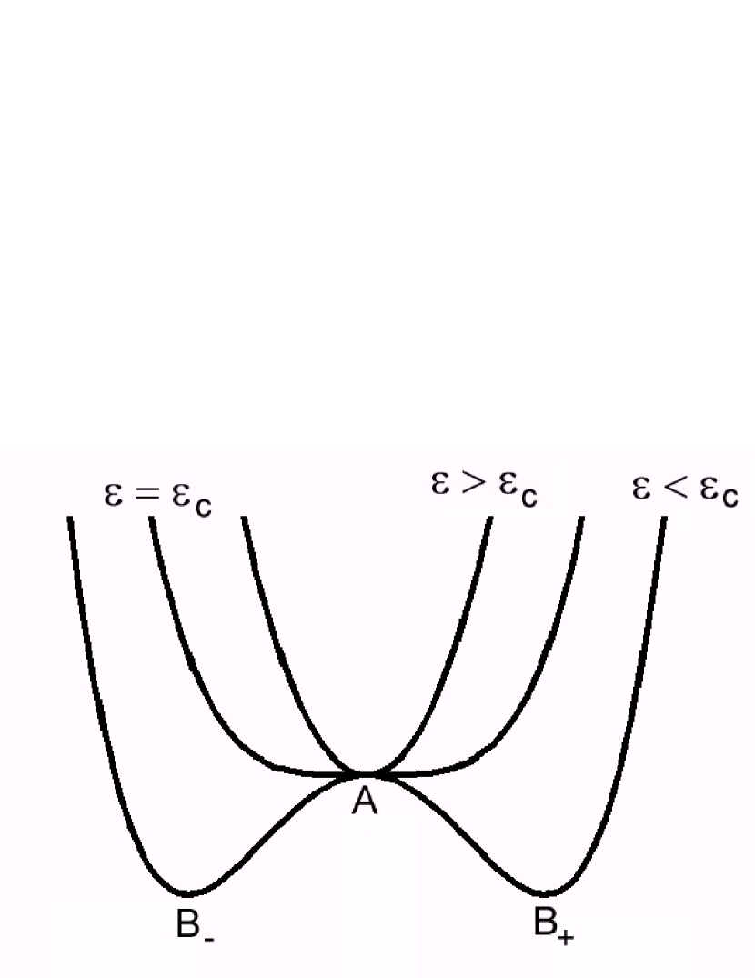
Figure 1: Potential energy $V$ as a function of the fundamental mode displacement $Y$. The shape of the potential energy is harmonic for $\varepsilon>\varepsilon_{c}$, quartic for $\varepsilon=\varepsilon_{c}\equiv$ critical strain ($\varepsilon_{c}<0$) and a double well for $\varepsilon<\varepsilon_{c}$.

The two minima in the potential energy curve describe the two possible buckled states at a particular strain Carr and the system can change from one state to the other, under thermal fluctuations or quantum tunneling. In our earlier publications Ani ; Sayan we have used multidimensional transition state theory (TST) to derive expressions for the transition rate from one potential well to the other. We now include the effect of friction on the reaction rate. For this, we follow the procedure Weiss used for the study of barrier crossing and other dynamical problems in the presence of friction.

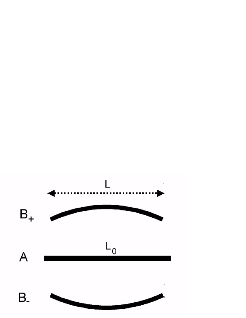
Figure 2: The rod under compression: The central figure (A) shows the uncompressed rod of length $L_{0}$. On compressing to length $L$, the rod buckle, either to $B_{-}$ or to $B_{+}$.

II The Model

We consider the normal modes and associated quantum properties of an elastic rectangular rod of length $L$, width $w$ and thickness $d$ (satisfying $L>>w>>d$) Carr ; Wybourne ; CarrAPL ; Lawrence . We assume that $d$ is smaller than $w$ so that transverse displacements $y(x)$ only occur in the “$d$ ” direction. $F$ is the linear modulus (energy per unit length) of the rod and is related to the elastic modulus $Q$ of the material by $F=Q$ $w$ $d$. The bending moment $\kappa$ is given by $\kappa^{2}=\frac{d^{2}}{12}$ for a rod of rectangular cross section and $\mu=\frac{m}{L}$ is the mass per unit length. We take the length of the rod (uncompressed) to be $L_{0}$. As in the Fig. 2, we apply compression on the two ends, reducing the separation between the two to $L$. Then if $y(x)$ denotes the displacement of the rod in the ‘$d$’ direction, the total potential energy is given by Sayan ; Ani

$$V[y(x)]=\frac{1}{2}\int\limits_{0}^{L}dx(F\kappa^{2}(y^{\prime\prime})^{2}+F\varepsilon(y^{\prime})^{2})+\frac{F}{8L_{0}}(\int\limits_{0}^{L}dx(y^{\prime})^{2})^{2}+\frac{FL_{0}}{2}\varepsilon^{2}.$$ (1)

In the above $\varepsilon=\frac{(L-L_{0})}{L_{0}}$ is the strain, negative if compressive. We imagine that each segment of the rod (labelled by $x$) is coupled to a collection of harmonic oscillators which form the reservoir. Each section has its own independent collection of harmonic oscillators. So the total system, rod plus the reservoir has the energy Sayan

$$H=\frac{1}{2}\int\limits_{0}^{L}dx\ \mu\stackrel{{\scriptstyle.}}{{y}}^{2}+V[y]+\frac{1}{2}\sum_{\alpha=1}^{N}\int\limits_{0}^{L}dx$$

$$\times\left\{m_{\alpha}(x)\stackrel{{\scriptstyle.}}{{\xi}}_{\alpha}^{2}+m_{\alpha}(x)\omega_{\alpha}^{2}(x)\left(\xi_{\alpha}(x)-\frac{c_{\alpha}(x)y(x)}{m_{\alpha}(x)\omega_{\alpha}^{2}(x)}\right)^{2}\right\}.$$ (2)

In the above, $\xi_{\alpha}(x)$ denotes the position of $(\alpha,x)$-th harmonic oscillator of the reservoir, coupled to $y(x)$, the displacement of the rod at location $x$. It has a frequency $\omega_{\alpha}(x)$ and mass $m_{\alpha}(x)$, $c_{\alpha}(x)$ determines the coupling of the $\xi_{\alpha}(x)$ to the $y(x)$. The way, the coupling has been chosen, the barrier height remains unchanged. Here $\alpha$ varies over the collection of harmonic oscillators, and we let $\alpha$ vary from $1$ to $N$.

III Quantum transition state theory in presence of friction

To derive the quantum rate we use the following methodology. The Hamiltonian given in Eq. (II) may be treated as a quantum Hamiltonian. For a finite discrete set of oscillators one may evaluate the quantum rate using quantum transition state theory under harmonic approximations. The quantum transition state theory rate expression is given by PollakCPL ; PollakPRA

$$R_{quantum}^{fric}=\frac{kT}{h}\left(\frac{\hbar\beta\Omega^{fric}}{2\sin(\frac{1}{2}\hbar\beta\Omega^{fric})}\right)\frac{Q^{\ddagger}}{Q}e^{-\beta E_{act}}.$$ (3)

In the above $Q^{\ddagger}$ and $Q$ are the partition function at the saddle point and at the reactant, and $\Omega^{fric}$ is the frequency of the ‘unstable mode’. Following Pollak PollakCPL , the quantum partition function at the saddle point

$$Q^{\ddagger}=\prod\limits_{n=2}^{\infty} \left(\frac{1}{2\sinh(\frac{1}{2}\hbar\beta\chi_{n}^{\ddagger})}\prod\limits_{j=1}^{N}\frac{1}{2\sinh(\frac{1}{2}\hbar\beta\lambda_{n,j}^{\ddagger})}\right).$$ (4)

At the saddle point we have $N\times N-1$ real oscillators and one imaginary oscillator. $\lambda_{nj}^{\ddagger}$ is the ‘bath’ frequency and $\chi_{n}^{\ddagger}$ is the ‘system’ frequency at the saddle point. Note the well known divergence of $Q^{\ddagger}$ at low temperatures. The quantum partition function at the reactant geometry

$$Q=\prod\limits_{n=1}^{\infty}\left(\frac{1}{2\sinh(\frac{1}{2}\hbar\beta\chi_{n})}\prod\limits_{j=1}^{N}\frac{1}{2\sinh(\frac{1}{2}\hbar\beta\lambda_{n,j})}\right).$$ (5)

In the above $\lambda_{n,j}$ is the ‘bath’ frequency and $\chi_{n}$ is the ‘system’ frequency at the reactant geometry.

IV The Extrema of the functional $V[y(x)]$

To find the equilibrium state, we extremise potential energy functional with respect to $y(x)$. For this we put $\frac{\delta V[y(x)]}{\delta y(x)}=0$. This leads to the differential equation

$$F\kappa^{2}\frac{\partial^{4}y}{\partial x^{4}}-[F\varepsilon\frac{\partial^{2}y}{\partial x^{2}}+\frac{F}{2L_{0}}(\int\limits_{0}^{L}dx(y^{\prime}(x))^{2})\frac{\partial^{2}y}{\partial x^{2}}]=0$$ (6)

and the hinged end points have boundary conditions $y(0)=y(L)=0$ and $y^{\prime\prime}(0)=y^{\prime\prime}(L)=0.$ The only solution to Eq. (6) is $y(x)=0$ if $\varepsilon>\varepsilon_{c},$ where $\varepsilon_{c}=-\frac{\kappa^{2}\pi^{2}}{L^{2}}.$ But if $\varepsilon<\varepsilon_{c}$ two more solutions are possible. They are given by

$$y(x)=\pm A\sqrt{\frac{2}{L}}\sin(\frac{\pi}{L}x).$$ (7)

On substituting Eq. (7) into Eq. (6), we find a nonlinear equation for $A$, which on solution gives

$$A=\sqrt{\frac{2L_{0}L^{2}}{\pi^{2}}(\varepsilon_{c}-\varepsilon)}.$$ (8)

These two are the buckled states which are minima of the potential energy surface for $\varepsilon<\varepsilon_{c}$, as all the normal modes around this are stable. The solution $y(x)=0$ is now a saddle point (see next section for details).

V Normal modes of the system Hamiltonian

We find the potential energy for the buckled states $E_{b}=-\frac{FL_{0}}{2}(\varepsilon-\varepsilon_{c})^{2}$. $y(x)=0$ is the straight rod configuration and is the saddle point for transition from one buckled state to the other. Its potential energy $E_{Saddle}^{Linear}$ is zero. One can calculate the barrier height for the process of going from one buckled state to the other as

$$\Delta E_{Barrier}^{Linear}=\frac{FL_{0}}{2}(\varepsilon-\varepsilon_{c})^{2}.$$ (9)

The kinetic energy of the rod is $\frac{\mu}{2}\int_{0}^{L}y_{t}^{2}dx$, where $\mu=\frac{m}{L_{0}}$ is the mass per unit length. We now look at small amplitude vibrations around each extremum $y_{ext}(x)$, which could be the buckled or the saddle point. One gets

$$\mu\frac{\partial^{2}\delta y(x,t)}{\partial t^{2}}=-\int\limits_{0}^{L}dx_{1}\left(\frac{\delta^{2}V[y(x)]}{\delta y(x_{1})\delta y(x)}\right)_{y_{ext}(x_{1})}\delta y(x_{1},t).$$ (10)

On evaluation we get

$$\mu\frac{\partial^{2}\delta y(x,t)}{\partial t^{2}}=-{\cal L}_{ext}\delta y(x,t),$$ (11)

where the operator ${\cal L}_{ext}$ is defined by

$${\cal L}_{ext}\delta y(x,t)= F\kappa^{2}\delta y^{\prime\prime\prime\prime}(x,t)-F\varepsilon\delta y^{\prime\prime}(x,t)-\frac{F}{2L_{0}}(\int\limits_{0}^{L}dx(y_{ext}^{\prime}(x))^{2})\delta y^{\prime\prime}(x,t)$$

$$+\frac{F}{L_{0}}y_{ext}^{\prime\prime}(x)(\int\limits_{0}^{L}dx_{1}\;y_{ext}^{\prime\prime}(x_{1})\delta y(x_{1},t)).$$ (12)

Using the boundary conditions for the hinged end points, we find the normal modes of the rod, $\delta y(x,t)=\delta y_{n}(x)e^{i\omega_{n}t}$. At the saddle point, $y_{ext}(x)=$ $y_{0}(x)=0$. Using this in Eq. (V), we obtain

$$\delta y_{n}(x)=A_{n}\sqrt{\frac{2}{L}}\sin(\frac{n\pi}{L}x),$$ (13)

with n=1,2,3…. The normal mode frequencies at the saddle point are given by ($\ddagger$ is used to denote the saddle point)

$$\,\omega_{Linear,n}^{\ddagger}=\omega_{0}\;n\,\sqrt{n^{2}-\frac{\varepsilon}{\varepsilon_{c}}}.$$ (14)

$\omega_{0}=\frac{\pi^{2}\kappa}{L^{2}}\sqrt{\frac{F}{\mu}}$. $n=1$ is the unstable mode and it has the imaginary frequency $\omega_{1}=i\Omega_{Linear}$, where

$$\Omega_{Linear}=\omega_{0}\;\,\sqrt{\frac{\varepsilon}{\varepsilon_{c}}-1}.$$ (15)

For small amplitude vibrations around the buckled state, one has to put $y_{ext}(x)=A\sqrt{\frac{2}{L}}\sin(\frac{\pi}{L}x)$. The normal modes are the same as in the Eq. (LABEL:B33), but the normal mode frequencies are different. They are

$$\omega_{n}=\omega_{0}n\sqrt{n^{2}-1}\qquad for\quad n>1,$$ (16)

while

$$\omega_{1}=\omega_{0}\sqrt{2\left(\frac{\varepsilon}{\varepsilon_{c}}-1\right)}.$$ (17)

V.1 The Rate near first buckling instability

The reaction rate using quantum transition state theory may be written as PollakCPL

$$R_{quantum,f}^{fric}=\rho_{f}(\frac{\omega_{1}}{2\pi})(\frac{\Omega^{fric}_{Linear}}{\Omega_{Linear}})\prod\limits_{n=2}^{\infty}\frac{\omega_{n}}{\omega_{Linear,n}^{\ddagger}}e^{-\beta\Delta E_{Barrier}^{Linear}},$$ (18)

where, we have used the following expression for $\Omega_{Linear}^{fric}$ Ani

$$\Omega_{Linear}^{fric}=-\frac{\gamma}{2}+\sqrt{\left(\frac{\gamma}{2}\right)^{2}+\omega_{0}^{2}\left(\frac{\varepsilon}{\varepsilon_{c}}-1\right)}$$ (19)

and the expression for $\rho$ is given by

$$\rho_{f}=\frac{\Omega_{Linear}}{\omega_{1}}\prod\limits_{n=2}^{\infty}\left(\frac{\omega_{Linear,n}^{\ddagger}}{\omega_{n}}\right)\frac{\sinh(\frac{1}{2}\hbar\beta\chi_{1})\prod\limits_{j=1}^{N}\frac{1}{2\sinh(\frac{1}{2}\hbar\beta\lambda_{n,j}^{\ddagger})}}{\sin(\frac{1}{2}\hbar\beta\Omega_{Linear}^{fric})\prod\limits_{j=1}^{N}\frac{1}{2\sinh(\frac{1}{2}\hbar\beta\lambda_{n,j})}}$$

$$\frac{\prod\limits_{n=2}^{\infty}\left(\frac{1}{2\sinh(\frac{1}{2}\hbar\beta\chi_{n}^{\ddagger})}\prod\limits_{j=1}^{N}\frac{1}{2\sinh(\frac{1}{2}\hbar\beta\lambda_{n,j}^{\ddagger})}\right)}{\prod\limits_{n=2}^{\infty}\left(\frac{1}{2\sinh(\frac{1}{2}\hbar\beta\chi_{n})}\prod\limits_{j=1}^{N}\frac{1}{2\sinh(\frac{1}{2}\hbar\beta\lambda_{n,j})}\right)}.$$ (20)

In the above $\omega_{n}$ and $\omega_{Linear,n}^{\ddagger}$ represents frequencies of normal modes of the system at reactant geometry and at the saddle point respectively in absence of bath. In case when the system is coupled to the bath $\lambda_{n,j}^{\ddagger}$ is the new ‘bath’ frequency and $\chi_{n}^{\ddagger}$ is the new ‘system’ frequency at the saddle point, also $\lambda_{n,j}$ is the new ‘bath’ frequency and $\chi_{n}$ is the new ‘system’ frequency at the reactant geometry. To evaluate $\rho$, we use the following two identities Ryzhik

$$\sinh(x)=x\prod\limits_{k=1}^{\infty}(1+\frac{x^{2}}{k^{2}\pi^{2}})$$ (21)

and

$$\sin(x)=x\prod\limits_{k=1}^{\infty}(1-\frac{x^{2}}{k^{2}\pi^{2}}).$$ (22)

Following Pallak PollakCPL one can prove the following identity

$$({-{\Omega^{fric}_{Linear}}^{2}+\epsilon^{2}})\prod\limits_{i=1}^{N}({\lambda_{1,i}^{\ddagger 2}+\epsilon^{2}})\times\prod\limits_{n=2}^{\infty}\left(({\chi_{n}^{\ddagger 2}+\epsilon^{2}})\prod\limits_{j=1}^{N}({\lambda_{n,j}^{\ddagger 2}+\epsilon^{2}})\right)$$

$$=\left({-\Omega_{Linear}^{2}+\epsilon^{2}+\epsilon\gamma}\right)\prod\limits_{\alpha=1}^{N}({\omega_{\alpha}^{2}+\epsilon^{2}})\times\prod\limits_{n=2}^{\infty}\left(({\omega_{Linear,n}^{\ddagger 2}+\epsilon^{2}})\prod\limits_{\alpha=1}^{N}({\omega_{\alpha}^{2}+\epsilon^{2}})\right),$$ (23)

where $\epsilon$ is an arbitrary number. Also

$$({{\chi_{1}}^{2}+\epsilon^{2}})\prod\limits_{i=1}^{N}({\lambda_{1,i}^{2}+\epsilon^{2}})\times\prod\limits_{n=2}^{\infty}\left(({\chi_{n}^{2}+\epsilon^{2}})\prod\limits_{j=1}^{N}({\lambda_{n,j}^{2}+\epsilon^{2}})\right)$$

$$=\left({\omega_{1}^{2}+\epsilon^{2}+\epsilon\gamma}\right)\prod\limits_{\alpha=1}^{N}({\omega_{\alpha}^{2}+\epsilon^{2}})\times\prod\limits_{n=2}^{\infty}\left(({\omega_{n}^{2}+\epsilon^{2}})\prod\limits_{\alpha=1}^{N}({\omega_{\alpha}^{2}+\epsilon^{2}})\right).$$ (24)

We use the notation $\nu=\frac{2\pi}{\hbar\beta}$. Insertion of Eq. (22) into Eq. (21) and use of Eq. (V.1) and Eq. (V.1) with $\epsilon=0$ gives

$$\rho_{f}= \left(\prod\limits_{k=1}^{\infty}\frac{(k^{2}\nu^{2}+\chi_{1}^{2})}{(k^{2}\nu^{2}-\Omega^{2}_{fric})}\right)\prod\limits_{i=1}^{N}\prod\limits_{k=1}^{\infty}\left(\frac{(k^{2}\nu^{2}+\lambda_{1,i}^{2})}{(k^{2}\nu^{2}+\lambda_{1,i}^{\ddagger 2})}\right)$$

$$\prod\limits_{n=2}^{\infty}\left(\left(\prod\limits_{k=1}^{\infty}\frac{(k^{2}\nu^{2}+\chi_{n}^{2})}{(k^{2}\nu^{2}+\chi_{n}^{\ddagger 2})}\right)\prod\limits_{i=1}^{N}\prod\limits_{k=1}^{\infty}\left(\frac{(k^{2}\nu^{2}+\lambda_{1,i}^{2})}{(k^{2}\nu^{2}+\lambda_{1,i}^{\ddagger 2})}\right)\right).$$ (25)

Interchanging the order of the products and using ratio of Eq. (V.1) and Eq. (V.1)with the identification $\epsilon=k\nu$ gives the desired result.

$$\rho_{f}=\left(\prod\limits_{k=1}^{\infty}\frac{(k^{2}\nu^{2}+\omega_{1}^{2}+\nu k\gamma)}{(k^{2}\nu^{2}-\Omega^{2}_{fric}+\nu k\gamma)}\right)$$

$$\prod\limits_{n=2}^{\infty}\left(\prod\limits_{k=1}^{\infty}\frac{(k^{2}\nu^{2}+\omega_{n}^{2}+\nu k\gamma)}{(k^{2}\nu^{2}+\omega_{Linear,n}^{\ddagger 2}+\nu k\gamma)}\right).$$ (26)

On simplification we get

$$\rho_{f}=\frac{\Gamma\left(\frac{\gamma+2\nu-\sqrt{\gamma^{2}+4\Omega^{2}_{Linear}}}{2\nu}\right)\Gamma\left(\frac{\gamma+2\nu+\sqrt{\gamma^{2}+4\Omega^{2}_{Linear}}}{2\nu}\right)}{\Gamma\left(\frac{\gamma+2\nu-\sqrt{\gamma^{2}-4(\omega_{1})^{2}}}{2\nu}\right)\Gamma\left(\frac{\gamma+2\nu+\sqrt{\gamma^{2}-4(\omega_{1})^{2}}}{2\nu}\right)}$$

$$\times\prod\limits_{n=2}^{\infty}\frac{\Gamma\left(\frac{\gamma+2\nu-\sqrt{\gamma^{2}-4(\omega_{Linear,n}^{\ddagger})^{2}}}{2\nu}\right)\Gamma\left(\frac{\gamma+2\nu+\sqrt{\gamma^{2}-4(\omega_{Linear,n}^{\ddagger})^{2}}}{2\nu}\right)}{\Gamma\left(\frac{\gamma+2\nu-\sqrt{\gamma^{2}-4(\omega_{n})^{2}}}{2\nu}\right)\Gamma\left(\frac{\gamma+2\nu+\sqrt{\gamma^{2}-4(\omega_{n})^{2}}}{2\nu}\right)}$$ (27)

VI Beyond the Second Buckling Instability

As $\sqrt{\frac{\varepsilon}{\varepsilon_{c}}}\rightarrow 2$, $\omega_{Linear,2}^{\ddagger}\rightarrow 0$ and the reaction rate diverges [see Eq. (18)]. So the rate expression in Eq. (18) is valid only if one is not too near $\sqrt{\frac{\varepsilon}{\varepsilon_{c}}}=2$. This is due to the setting in of the second buckling instability. As the rod is compressed, first the mode $A_{1}\sqrt{\frac{2}{L}}\sin(\frac{\pi}{L}x)$ becomes unstable and this is the first buckling instability and the rod buckles as a result of this. The length at which this occurs shall be denoted by $L_{f}$. If one supposes that the rod is compressed further keeping the straight rod configuration, then at a length $L_{s}$, the mode $A_{2}\sqrt{\frac{2}{L}}\sin(\frac{2\pi}{L}x)$ too would become unstable and this is the second buckling instability. What happens here is a reaction path bifurcation for the crossing from one buckled state to the other and is very interesting. For $\varepsilon>4\varepsilon_{c}$, there is only one saddle point but for $\varepsilon<4\varepsilon_{c}$, this saddle point bifurcates into two and consequently the calculation of rate near the bifurcation is a challenging problem. In a similar fashion one can have the third instability at a length $L_{t}$ etc. but these present no problem as far as rate calculation is concerned (see below). In order to analyze the rate near and beyond the second buckling instability, we proceed as follows. We assume that the Eq. (12) has solutions of the form

$$y_{0}(x)=A_{1}\sqrt{\frac{2}{L}}\sin(\frac{\pi}{L}x)+A_{2}\sqrt{\frac{2}{L}}\sin(\frac{2\pi}{L}x).$$ (28)

Using this, the elastic potential energy is given by

$$V[A_{1},A_{2}]= \frac{F\pi^{4}(A_{1}^{2}+4A_{2}^{2})^{2}}{8L^{4}L_{0}}+\frac{F\pi^{2}A_{1}^{2}(\varepsilon-\varepsilon_{c})}{2L^{2}}$$

$$+\frac{2F\pi^{2}A_{2}^{2}(\varepsilon-4\varepsilon_{c})}{L^{2}}.$$ (29)

The two buckling instabilities are clearly evident from this expression - as each the coefficient of $A_{1}^{2}$ or $A_{2}^{2}$ changes sign from positive to negative. Finding the extrema of this potential leads to the following solutions for ($A_{1}$, $A_{2}$)

1. ($0$, $0$): this is the straight rod configuration. Between first and second buckling (i.e. $L_{s}<L<L_{f}$ ), this is the saddle point. But after the second buckling, it is no longer a saddle, but it becomes a hill top. It has an energy $E_{hilltop}=0$.

2. ($\pm\frac{2}{\pi}\sqrt{LL_{0}(\varepsilon_{c}-\varepsilon)}$, $0$): These are the buckled states and both of them have the same energy $E_{b}=-\frac{FL_{0}}{2}(\varepsilon-\varepsilon_{c})^{2}$.

3. ($0$, $\pm\frac{1}{\pi}\sqrt{LL_{0}(4\varepsilon_{c}-\varepsilon)}$): These are the two new saddle points that arise from the bifurcation of the one that existed for $4\varepsilon_{c}>\varepsilon$. These two have the same energy $E_{saddle}^{Bent}=-\frac{FL_{0}}{2}(\varepsilon-4\varepsilon_{c})^{2}$. At these saddle points, the rod has a bent (S-shaped) geometry. Beyond the second buckling instability, the barrier height is given by

$$\Delta E_{Barrier}^{Bent}=-\frac{3FL_{0}\varepsilon_{c}}{2}(-2\varepsilon+5\varepsilon_{c}).$$ (30)

Beyond the second buckling instability, away from the instability, one can do a normal mode analysis near the vicinity of the new saddles - there are two of them, both making identical contributions to the reaction rate. Near the buckled state, the normal modes have the frequencies given in the Eq. (16) and Eq. (17), while near the saddle, the frequencies are given by

$$\omega_{Bent,1}^{\ddagger}=\Omega_{Bent},$$ (31)

$$\omega_{Bent,2}^{\ddagger}=\omega_{0}\sqrt{8(\frac{\varepsilon}{\varepsilon_{c}}-4)},$$ (32)

$$\omega_{Bent,n}^{\ddagger}=\omega_{0}n\sqrt{n^{2}-4},$$ (33)

for $n>2$. In the above $\omega_{Bent,1}^{\ddagger}$ and has an imaginary frequency with

$$\Omega_{Bent}=\sqrt{3}\omega_{0}.$$ (34)

Now the quantum rate beyond the second buckling instability can be calculated taking the saddle to be the bent configuration.

$$R_{quantum,s}^{fric}=2\times\rho_{s}(\frac{\omega_{1}}{2\pi})(\frac{\Omega^{fric}_{Bent}}{\Omega_{Bent}})\prod\limits_{n=2}^{\infty}\frac{\omega_{n}}{\omega_{Bent,n}^{\ddagger}}e^{-\beta\Delta E_{Barrier}^{Bent}},$$ (35)

where, we have used the following expression for $\Omega_{Bent}^{fric}$ Ani

$$\Omega_{Bent}^{fric}=-\frac{\gamma}{2}+\sqrt{\left(\frac{\gamma}{2}\right)^{2}+3\omega_{0}^{2}}$$ (36)

and the expression for $\rho_{s}$ is given by

$$\rho_{s}=\frac{\Gamma\left(\frac{\gamma+2\nu-\sqrt{\gamma^{2}+4\Omega^{2}_{Bent}}}{2\nu}\right)\Gamma\left(\frac{\gamma+2\nu+\sqrt{\gamma^{2}+4\Omega^{2}_{Bent}}}{2\nu}\right)}{\Gamma\left(\frac{\gamma+2\nu-\sqrt{\gamma^{2}-4(\omega_{1})^{2}}}{2\nu}\right)\Gamma\left(\frac{\gamma+2\nu+\sqrt{\gamma^{2}-4(\omega_{1})^{2}}}{2\nu}\right)}$$

$$\times\prod\limits_{n=2}^{\infty}\frac{\Gamma\left(\frac{\gamma+2\nu-\sqrt{\gamma^{2}-4(\omega_{Bent,n}^{\ddagger})^{2}}}{2\nu}\right)\Gamma\left(\frac{\gamma+2\nu+\sqrt{\gamma^{2}-4(\omega_{Bent,n}^{\ddagger})^{2}}}{2\nu}\right)}{\Gamma\left(\frac{\gamma+2\nu-\sqrt{\gamma^{2}-4(\omega_{n})^{2}}}{2\nu}\right)\Gamma\left(\frac{\gamma+2\nu+\sqrt{\gamma^{2}-4(\omega_{n})^{2}}}{2\nu}\right)}$$ (37)

We have multiplied the quantum rate by a factor of 2 to account for the fact that there are two saddles of equal energy. It is interesting that the normal modes for this saddle retain their stability, irrespective of what the compression is. The first mode is always unstable and other modes always stable for all values of $\epsilon$. Therefore, this rate expression is valid for all values of $\epsilon<4\epsilon_{c}$ - that is even through the third buckling instability.

VI.1 The rate near second buckling instability

Near the second buckling instability ($\sqrt{\frac{\varepsilon}{\varepsilon_{c}}}\rightarrow 2$), both $\omega_{Linear,2}^{\ddagger}$ and $\omega_{Bent,2}^{\ddagger}$ vanishes, causing the rate to diverge [see Eq. (18) and Eq. (35)]. The cure for this divergence is to go beyond the harmonic approximations for the first two modes. Our discussion here follows that of Weiss Weiss . For the model described by the Hamiltonian

$$H=\frac{1}{2}\int\limits_{0}^{L}dx\ \mu\stackrel{{\scriptstyle.}}{{y}}^{2}+V[y]+\frac{1}{2}\sum_{\alpha}\int\limits_{0}^{L}dx$$

$$\times\left\{m_{\alpha}(x)\stackrel{{\scriptstyle.}}{{\xi}}_{\alpha}^{2}+m_{\alpha}(x)\omega_{\alpha}^{2}(x)\left(\xi_{\alpha}(x)-\frac{c_{\alpha}(x)y(x)}{m_{\alpha}(x)\omega_{\alpha}^{2}(x)}\right)^{2}\right\}.$$ (38)

We note that $m_{\alpha}(x)$ is independent of $x$ and may be written as $m_{\alpha}$, $\omega_{\alpha}^{2}(x)$ too, as well as $c_{\alpha}(x)$. So we can write the above expression as

$$H=\frac{1}{2}\int\limits_{0}^{L}dx\mu\stackrel{{\scriptstyle.}}{{y}}^{2}+V[y]+$$

$$\frac{1}{2}\sum\limits_{\alpha}\int dx\left\{m_{\alpha}\stackrel{{\scriptstyle.}}{{\xi}}_{\alpha}^{2}(x)+m_{\alpha}\omega_{\alpha}^{2}\left(\xi_{\alpha}(x)-\frac{c_{\alpha}y(x)}{m_{\alpha}\omega_{\alpha}^{2}}\right)^{2}\right\}.$$ (39)

Now let

$$\xi_{\alpha}(x)=\sum\limits_{n}\sqrt{\frac{2}{L}}\xi_{\alpha,n}\sin(\frac{n\pi x}{L})$$ (40)

and

$$y(x)=\sum\limits_{n}\sqrt{\frac{2}{L}}A_{n}\sin(\frac{n\pi x}{L}).$$ (41)

Then,

$$H=\frac{1}{2}\mu\sum\limits_{n}\stackrel{{\scriptstyle.}}{{y_{n}}}^{2}+V[A_{1},A_{2},....A_{n}]$$

$$+\frac{1}{2}\sum\limits_{\alpha,n}\left\{m_{\alpha}\stackrel{{\scriptstyle.}}{{\xi}}_{\alpha,n}^{2}+m_{\alpha}\omega_{\alpha}^{2}\left(\xi_{\alpha,n}-\frac{c_{\alpha}A_{n}}{m_{\alpha}\omega_{\alpha}^{2}}\right)^{2}\right\},$$ (42)

which decouples all the modes. The Hamiltonian for the first two modes coupled with bath is given by

$$E=\frac{1}{2}\mu\left(\stackrel{{\scriptstyle.}}{{A_{1}}}^{2}+\stackrel{{\scriptstyle.}}{{A_{2}}}^{2}\right)+V[A_{1},A_{2}]$$

$$+\frac{1}{2}\sum\limits_{\alpha}\{m_{\alpha}\stackrel{{\scriptstyle.}}{{\xi}}_{\alpha,1}^{2}+m_{\alpha}\stackrel{{\scriptstyle.}}{{\xi}}_{\alpha,2}^{2}+m_{\alpha}\omega_{\alpha}^{2}\left(\xi_{\alpha,1}-\frac{c_{\alpha}A_{1}}{m_{\alpha}\omega_{\alpha}^{2}}\right)^{2}$$

$$+m_{\alpha}\omega_{\alpha}^{2}\left(\xi_{\alpha,2}-\frac{c_{\alpha}A_{2}}{m_{\alpha}\omega_{\alpha}^{2}}\right)^{2}\}$$ (43)

In the Euclidean action ($S^{(E)}$) contains contributions from the system ($S_{S}^{(E)}$), the reservoir ($S_{R}^{(E)}$) and the interaction ($S_{I}^{(E)}$),

$$S^{(E)} =S_{S}^{(E)}+S_{R}^{(E)}+S_{I}^{(E)}$$

$$=S_{S}^{(E)}+\int\limits_{0}^{\beta\hbar}d\tau(L_{R}^{(E)}+L_{I}^{(E)})$$ (44)

with

$$S_{S}^{(E)}= S_{opt}=\int\limits_{0}^{\beta\hbar}d\tau\{\frac{1}{2}\mu\left(\frac{dA_{1}(\tau)}{d\tau}\right)^{2}-\frac{1}{2}\mu\Omega^{2}A_{1}^{2}(\tau)$$

$$+\frac{1}{2}\mu\left(\frac{dA_{2}(\tau)}{d\tau}\right)^{2}+\frac{1}{2}\mu\omega_{2}^{2}(\overline{A}_{2})(A_{2}(\tau)-\overline{A}_{2})^{2}$$

$$+L_{2}(\overline{A}_{2})\}.$$ (45)

In this optimized action two modes are decoupled. Also

$$L_{R}^{(E)}=\sum\limits_{\alpha=1}^{N}\frac{1}{2}m_{\alpha}(\overset{.}{\xi}_{\alpha,1}^{2}+\omega_{\alpha}^{2}{{\xi}_{\alpha,1}}^{2}+\overset{.}{\xi}_{\alpha,2}^{2}+\omega_{\alpha}^{2}{{\xi}_{\alpha,2}}^{2})$$ (46)

$$L_{I}^{(E)}=\sum\limits_{\alpha=1}^{N}(-c_{\alpha}\xi_{\alpha,1}A_{1}+\frac{1}{2}\frac{c_{\alpha}^{2}A_{1}^{2}}{m_{\alpha}\omega_{\alpha}^{2}}-c_{\alpha}\xi_{\alpha,2}A_{2}+\frac{1}{2}\frac{c_{\alpha}^{2}A_{2}^{2}}{m_{\alpha}\omega_{\alpha}^{2}})$$ (47)

Now we write Euclidean action for the two modes (with bath) separately. For the first mode

$$S_{1}^{(E)}=\int\limits_{0}^{\beta\hbar}d\tau\{\frac{1}{2}\mu\left(\frac{dA_{1}(\tau)}{d\tau}\right)^{2}-\frac{1}{2}\mu\Omega^{2}A_{1}^{2}(\tau)$$

$$+\sum\limits_{\alpha=1}^{N}\{\frac{1}{2}m_{\alpha}(\overset{.}{\xi}_{\alpha,1}^{2}+\omega_{\alpha}^{2}{{\xi}_{\alpha,1}}^{2})-c_{\alpha}\xi_{\alpha,1}A_{1}+\frac{1}{2}\frac{c_{\alpha}^{2}A_{1}^{2}}{m_{\alpha}\omega_{\alpha}^{2}}\}\}$$ (48)

and for the second mode

$$S_{2}^{(E)}=\int\limits_{0}^{\beta\hbar}d\tau\{\frac{1}{2}\mu\left(\frac{dA_{2}(\tau)}{d\tau}\right)^{2}$$

$$+\frac{1}{2}\mu\omega_{2}^{2}(\overline{A}_{2})(A_{2}(\tau)-\overline{A}_{2})^{2}+L_{2}(\overline{A}_{2})$$

$$+\sum\limits_{\alpha=1}^{N}\{\frac{1}{2}m_{\alpha}(\overset{.}{\xi}_{\alpha,2}^{2}+\omega_{\alpha}^{2}{{\xi}_{\alpha,2}}^{2})-c_{\alpha}\xi_{\alpha,2}A_{2}+\frac{1}{2}\frac{c_{\alpha}^{2}A_{2}^{2}}{m_{\alpha}\omega_{\alpha}^{2}}\}\}$$ (49)

The expression for $S_{1}^{(E)}$ is equivalent to the expression for an inverted parabolic potential coupled to $N$ harmonic oscillatore. So we have a system of ($N+1$) harmonic oscillators and we can calculate $\Omega^{fric}$ using the method discussed in the classical calculation Sayan . Now we will calculate the partition function using the ‘action’ defined in Eq. (VI.1). Following Weiss Weiss we define “influence action” $S_{R,I}^{(E)}(A_{2},\bm{\xi})$, which captures the influence of the environment on the equilibrium properties of the open system.

$$S_{2}^{(E)}=S_{R,I}^{(E)}[A_{2},{\bm{\xi}}]=S_{R}^{(E)}[{\bm{\xi}}]+S_{I}^{(E)}[A_{2},{\bm{\xi}}]$$ (50)

The stationary paths of action, which we denote by $\overline{A}_{2}$ and by $\overline{\xi}_{\alpha,2}$, obey the Euclidean classical equations of motion

$$\mu\overset{..}{\overline{A_{2}}}-\frac{\partial V(\overline{A}_{2})}{\partial\overline{A_{2}}}+\sum\limits_{\alpha=1}^{N}c_{\alpha}(\overline{\xi}_{\alpha,2}-\frac{c_{\alpha}\overline{A}_{2}}{m_{\alpha}\omega_{\alpha}^{2}})=0$$

$$m_{\alpha}\overset{..}{\overline{\xi}}_{\alpha,2}-m_{\alpha}\omega_{\alpha}^{2}\overline{\xi}_{\alpha,2}+c_{\alpha}\overline{A}_{2}=0$$ (51)

We choose for convenience to periodically continue the paths $\xi_{\alpha,2}(\tau)$, $A_{2}(\tau)$ outside the range $0\leq\tau<\beta\hbar$ by writing them as Fourier series

$$\xi_{\alpha,2}(\tau)=\sum\limits_{n=-\infty}^{n=\infty}\xi_{\alpha,2,n}e^{i\nu_{n}\tau}$$

$$A_{2}(\tau)=\sum\limits_{n=-\infty}^{n=\infty}A_{2,n}e^{i\nu_{n}\tau}$$ (52)

where $\xi_{\alpha,2,n}=\xi_{\alpha,2,-n}^{*}$, $A_{2,n}^{*}=A_{2,-n}^{*}$ and $\nu_{n}=\frac{2\pi n}{\beta\hbar}$ is a bosonic Matsubara frequency. Substituting Eq. (VI.1) into Eq. (50) and Eq. (46), we obtain

$$S_{R,I}^{(E)}[A_{2},{\bm{\xi}}]= \sum\limits_{\alpha=1}^{N}{\beta\hbar}\sum\limits_{n=-\infty}^{n=\infty}\frac{m_{\alpha}}{2}$$

$$(\nu_{n}^{2}\left|\xi_{\alpha,2,n}\right|^{2}+\omega_{\alpha}^{2}\left|\xi_{\alpha,2,n}-\frac{c_{\alpha}}{m_{\alpha}\omega_{\alpha}^{2}}A_{2,n}\right|^{2}).$$ (53)

Next, we decompose $\xi_{\alpha,2,n}$ into classical term $\overline{\xi}_{\alpha,2,n}$ and a deviation $y_{\alpha,2,n}$ describing quantum fluctuations,

$$\xi_{\alpha,2,n} =\overline{\xi}_{\alpha,2,n}+y_{\alpha,2,n}$$

$$=\frac{c_{\alpha}}{m_{\alpha}(\nu_{n}^{2}+\omega_{\alpha}^{2})}A_{2,n}+y_{\alpha,2,n}.$$ (54)

Figure 3: Plot of logarithm of rate of crossing from one buckled state to the other using quantum transition state theory without friction (solid line) and with friction (dashed line), for a Si rod of dimensions $L_{0}=500\>\AA$,$w=20\>\AA$, $d=10\>\AA$, $\gamma=1\times 10^{11}sec^{-1}$ and $T=0.01\>K$. For this rod the first three instabilities occur at $L_{f}-L_{0}=-0.1646\>\AA$, $L_{s}-L_{0}=-0.6597\>\AA$ and $\gamma=1\times 10^{11}sec^{-1}$.

In the second form, we have used the solution of the oscillator mode $\xi_{\alpha,2,n}$ following from Eq. (VI.1). Since $\xi_{\alpha,2}(\tau)$ is a stationary point of action, the term linear in the deviation is eliminated and we find an expression in which the quadratic forms of $\bm{y}$ and $A_{2}$ are decoupled,

$$S_{R,I}^{(E)}[A_{2},{\bm{\overline{\xi}}+{\bm{y}}}]=S_{R,I}^{(E)}[{\bm{y}}]+S_{\inf l}^{(E)}[A_{2}],$$ (55)

$$S_{R,I}^{(E)}[{\bm{y}}] =\sum\limits_{\alpha=1}^{N}{{\beta\hbar}}\sum\limits_{n=-\infty}^{n=\infty}\frac{m_{\alpha}}{2}(\nu_{n}^{2}+\omega_{\alpha}^{2})\left|y_{\alpha,2,n}\right|^{2}$$

$$=\sum\limits_{\alpha=1}^{N}\int\limits_{0}^{\beta\hbar}d\tau\frac{m_{\alpha}}{2}(\overset{.}{y}_{\alpha,2}^{2}+\omega_{\alpha}^{2}y_{\alpha,2}^{2}),$$ (56)

$$S_{infl}^{(E)}[A_{2}]=\sum\limits_{\alpha=1}^{N}{{\beta\hbar}}\frac{c_{\alpha}^{2}}{2m_{\alpha}}\sum\limits_{n=-\infty}^{n=\infty}\left(\frac{\left|A_{2,n}\right|^{2}}{\omega_{\alpha}^{2}}-\frac{\left|A_{2,n}\right|^{2}}{(\nu_{n}^{2}+\omega_{\alpha}^{2})}\right).$$ (57)

In the Fourier series representation, the influence action (Eq. (57)) takes the complete form

$$S_{infl}^{(E)}[A_{2}]={\mu}{\beta\hbar}\sum\limits_{n=-\infty}^{n=\infty}(\zeta_{n}\left|A_{2,n}\right|^{2}),$$ (58)

where

$$\zeta_{n} =\frac{1}{\mu}\sum\limits_{\alpha=1}^{N}\frac{c_{\alpha}^{2}}{2m_{\alpha}}\frac{\nu_{n}^{2}}{(\nu_{n}^{2}+\omega_{\alpha}^{2})}$$

$$=\frac{2}{\mu\pi}\frac{1}{\beta\hbar}\int\limits_{0}^{\infty}d\omega\frac{J(\omega)}{\omega}\frac{\nu_{n}^{2}}{(\nu_{n}^{2}+\omega^{2})}.$$ (59)

Assuming Ohmic friction Weiss

$$\zeta_{n}=\nu_{n}\gamma.$$ (60)

We want to calculate the ratio of partition functions for the second mode at the saddle and at the reactant geometry. As all other modes are harmonic, there contributions to the rate is calculated using the same procedure as discussed in the section 3.1. In our calculation we use the ‘action’ for the second mode at the saddle point, given in the Eq. (VI.1). Expanding the kinetic term into its Fourier components, we get

$$S_{2}^{(E)}=\mu\beta\hbar\left[\sum\limits_{n=1}^{\infty}(\nu_{n}^{2}+\omega_{2}^{2}(\overline{A}_{2})+\nu_{n}\gamma)\left|A_{2,n}\right|^{2}+L_{2}(\overline{A}_{2})\right]$$ (61)

So the partition function for the second mode at the saddle point is given by

$$Q_{2}^{\ddagger}= \int\limits_{-\infty}^{\infty}\frac{d\overline{A}_{2}e^{-\frac{L_{2}(\overline{A}_{2})}{kT}}}{\sqrt{2\pi\beta\hbar^{2}/\mu}}\Gamma[\frac{\beta\hbar}{4\pi}(\frac{4\pi}{\beta\hbar}+\gamma-\sqrt{\gamma^{2}-4\omega_{2}^{2}(\overline{A}_{2})})]$$

$$\times\Gamma[\frac{\beta\hbar}{4\pi}(\frac{4\pi}{\beta\hbar}+\gamma+\sqrt{\gamma^{2}-4\omega_{2}^{2}(\overline{A}_{2})})]\times Q_{bath}.$$ (62)

We have already determined $\Omega^{2}$, $\omega_{2}^{2}(\overline{A}_{2})$ and $L_{2}(\overline{A}_{2})$ variationally in the absence of reservoir. For the second mode at the reactant geometry, the expression for the partition function is given below

$$Q_{2}= \int\limits_{-\infty}^{\infty}\frac{d\overline{A}_{2}e^{-\frac{\mu\omega_{2}^{2}\overline{A}_{2}^{2}}{2kT}}}{\sqrt{2\pi\beta\hbar^{2}/\mu}}\Gamma[\frac{\beta\hbar}{4\pi}(\frac{4\pi}{\beta\hbar}+\gamma-\sqrt{\gamma^{2}-4\omega_{2}^{2}})]$$

$$\times\Gamma[\frac{\beta\hbar}{4\pi}(\frac{4\pi}{\beta\hbar}+\gamma+\sqrt{\gamma^{2}-4\omega_{2}^{2}})]\times Q_{bath}.$$ (63)

In the regime where $L>L_{s}$, the rate may be calculated using (transition state is assumed to be straight rod)

$$R_{quantum,i}^{fric}=\rho_{f}(\frac{\omega_{1}}{2\pi})(\frac{\Omega^{fric}_{Linear}}{\Omega_{Linear}}){\frac{Q_{2}^{\ddagger}}{Q_{2}}}\prod\limits_{n=3}^{\infty}\frac{\omega_{n}}{\omega_{Linear,n}^{\ddagger}}e^{-\beta\Delta E_{Barrier}^{Linear}}.$$ (64)

In the regime where $L<L_{s}$, the rate may be calculated using (transition state is assumed to be bent rod)

$$R_{quantum,i}^{fric}=\rho_{s}(\frac{\omega_{1}}{2\pi})(\frac{\Omega^{fric}_{Bent}}{\Omega_{Bent}}){\frac{Q_{2}^{\ddagger}}{Q_{2}}}\prod\limits_{n=3}^{\infty}\frac{\omega_{n}}{\omega_{Bent,n}^{\ddagger}}e^{-\beta\Delta E_{Barrier}^{Bent}}.$$ (65)

Figure 4: Plot of logarithm of rate of crossing from one buckled state to the other using quantum transition state theory without friction (solid line) and with friction (dashed line), for a Si rod of dimensions $L_{0}=500\>\AA$,$w=20\>\AA$, $d=10\>\AA$ and $T=30\>K$. For this rod the first three instabilities occur at $L_{f}-L_{0}=-0.1646\>\AA$, $L_{s}-L_{0}=-0.6597\>\AA$ and $\gamma=1\times 10^{11}sec^{-1}$.

VII Results

We now use the above formulae to calculate the rate of passage from one buckled state to the other, for $Si$ rod of dimensions $L_{0}=500\>\AA$,$w=20\>\AA$, $d=10\>\AA$, the case considered by Carr et al. Carr . The Young’s modulus and density of $Si$ are $Q=130\>GPa$ and $\rho=5000\>kg.m^{-3}$. The first and second buckling instabilities occur at lengths which we denote as $L_{f}$ and $L_{s}$ respectively and their values are given by $L_{f}-L_{0}=-0.1646\>\AA$, $L_{s}-L_{0}=-0.6597\>\AA$. In the regime $L\geq L_{s}$, the saddle point has straight rod configuration and in the regime $L<L_{s}$, the saddle point has bent configuration. At $T=0.01\>K$ we do not show the rate calculated near the second buckling instability - as it is extremely low (Fig. 3). The equations for rates have product over all the infinite modes, as would be normal for a continuum model. This however is not realistic, and this can be easily modified to account for discreteness of these rod. We do this, by restricting the product to contain just the same number of normal modes as the perpendicular degrees of freedom for the discrete model. We have thus taken contributions from first $2128$ normal modes of the rod. Fig. 4 shows the quantum rate against compression, made at a temperature of $30\>K$. Our calculation including friction shows that friction lowers rate of conversion from one buckled state to the other.

VIII Summary and Conclusions

In this paper we have discussed the buckling of a nano rod under compression and rate of it’s conversion from one buckled state to the other using quantum version of multidimensional transition state theory. As compression increases, the rod buckles (first buckling instability), and has now two stable states. From one stable state it can go over to the other by thermal fluctuations or quantum tunneling. Using a continuum approach, we have calculated the rate of conversion from one state to the other using system plus reservoir model. The saddle point for the change from one state to the other is the straight rod configuration. The rate expression, however, diverges at the second buckling instability. At this point, the straight rod configuration, which was a saddle till then, becomes hill top and two new saddles are generated. The new saddles have bent configurations and as the rod goes through further instabilities, they remain stable and the rate calculated according to the harmonic approximation around the saddle point remains finite. However, this rate too, diverges near the second buckling instability. In the quantum transition state theory calculation we have calculated centroid partition function for the second mode, and derived expressions that are well behaved through the second buckling instability. Using these expressions, we have calculated the rates for nano-rods of dimensions $L_{0}=500\>\AA$,$w=20\>\AA$, $d=10\>\AA$.

References

- (1) M. Roukes, Scientific American, September, 48 (2001).
- (2) H. G. Craighead, Science, 290 (2000) 1532.
- (3) H. Park, J. Park, A. K. L. Lim, E. H. Anderson, A. P. Alivisatos, and P. L. McEuen, Nature, 407 (2000) 57.
- (4) A. Erbe, R. H. Blick, A. Tilke, A. Kriele, and J. P. Kotthaus, Appl. Phys. Lett. 73 (1998) 3751.
- (5) A. N. Cleland and M. L. Roukes, Appl. Phys. Lett. 69 (1996) 2653.
- (6) T. Rueckes, K. Kim, E. Joselevich, G. Y. Tsewng, C. L. Cheung, and C. M. Lieber, Science, 289 (2000) 94.
- (7) S. M. Carr, W. E. Lawrence, and M. N. Wybourne, Phys. Rev. B 64 (2001) 220101(R).
- (8) L. Euler, in Elastic Curves, translated and annotated by W. A. Oldfather, C. A. Ellis, and D. M. Brown, reprinted from ISIS No. 58 XX(1), 1774 (Saint Catherine Press, Bruges, Belgium).
- (9) P. Hanggi, P. Talkner, and M. Borkovec, Rev. Mod. Phys. 62 (1990) 251.
- (10) A. Chakraborty, S. Bagchi and K. L. Sebastian, J. Comput. Theor. Nanosci. 4 (2007) 1.
- (11) A. Chakraborty, Mol. Phys. 107 (2009) 1777.
- (12) U. Weiss, Quantum Dissipative Systems, Series in Modern Condensed Matter Physics (World Scientific, Singapore, 1998).
- (13) S. M. Carr, W. E. Lawrence, and M. N. Wybourne, Physica B 316 (2002) 464.
- (14) S. M. Carr and M. N. Wybourne, Appl. Phys. Lett. 82 (2003) 709.
- (15) W. E. Lawrence, Physica B 316-317 (2002) 448.
- (16) Eli Pollak, Chem. Phys. Lett. 127 (1986) 178.
- (17) Eli Pollak, Phys. Rev. A 33 (1986) 4244.
- (18) I. S. Gradshteyn and I. M. Ryzhik, Table of integrals, series and products 4th Ed. (Academic Press, New York, 1980).