Hierarchical structures in the Large and Small Magellanic Clouds

Abstract

We investigate the degree of spatial correlation among extended structures in the LMC and SMC. To this purpose we work with sub-samples characterised by different properties such as age and size, taken from the updated catalogue of Bica et al. or gathered in the present work. The structures are classified as star clusters or non-clusters (basically, nebular complexes and their stellar associations). The radius distribution functions follow power-laws ($dN/dR\propto R^{-\alpha}$) with slopes and maximum radius ($R_{max}$) that depend on object class (and age). Non-clusters are characterised by $\alpha\approx 1.9$ and $R_{max}\la 472$ pc, while young clusters (age $\la 10$ Myr) have $\alpha\approx 3.6$ and $R_{max}\la 15$ pc, and old ones (age $\ga 600$ Myr) have $\alpha\approx 2.5$ and $R_{max}\la 40$ pc. Young clusters present a high degree of spatial self-correlation and, especially, correlate with star-forming structures, which does not occur with the old ones. This is consistent with the old clusters having been heavily mixed up, since their ages correspond to several LMC and SMC crossing times. On the other hand, with ages corresponding to fractions of the respective crossing times, the young clusters still trace most of their birthplace structural pattern. Also, small clusters ($R<10$ pc), as well as small non-clusters ($R<100$ pc), are spatially self-correlated, while their large counterparts of both classes are not. The above results are consistent with a hierarchical star-formation scenario for the LMC and SMC.

1 Introduction

Star formation in the Milky Way and other galaxies is described as a (mass and size) scale-free, hierarchical process, in which turbulent gas forms large-scale structures with a mass distribution following a power-law. In essence, such a scale-free process leads to a mass and size fractal distribution. As a consequence, young stellar groupings are clustered according to hierarchical patterns, with the great star complexes (associated with the $\sim 10^{7}\,\mbox{$M_{\odot}$}$ superclouds) at the largest scales and the OB associations and subgroups, small loose groups, clusters and cluster subclumps (e.g. Efremov 1995) at the smallest.

In several galaxies, the interstellar gas appears to follow a fractal structure ranging from the subpc ($\approx$ the current resolution limit) to the kpc scales; if star formation occurs preferentially at the densest regions, stars should form following such patterns (e.g. Elmegreen & Elmegreen 2001 and references therein). In this context, star clusters, formed at the core (i.e. the densest regions) of giant molecular clouds, can be taken as the unavoidable star formation product in a hierarchically structured gas (e.g. Elmegreen 2006). A similar picture, in which star clusters are present in dense cores, emerges from numerical simulations that follow in time the collapse of gas clouds (e.g. Walsh, Bourke & Myers 2006), which also occurs when effects of radiative feedback and magnetic fields are included (Bate 2009).

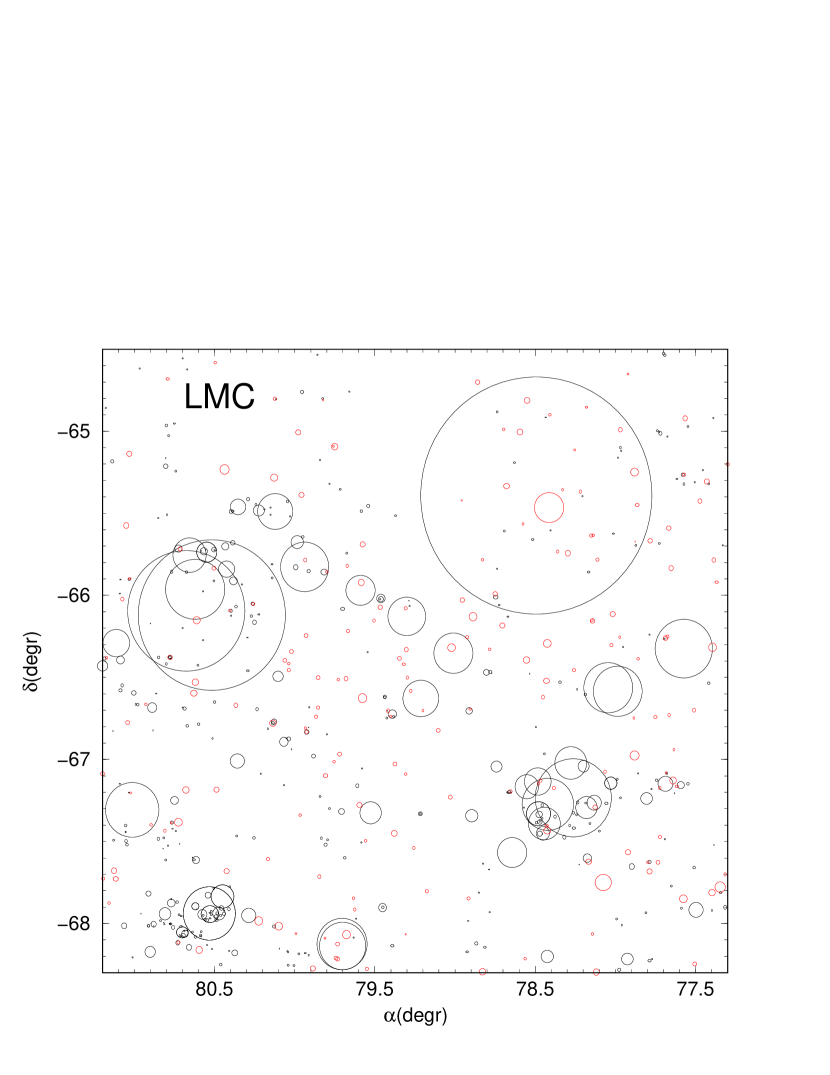
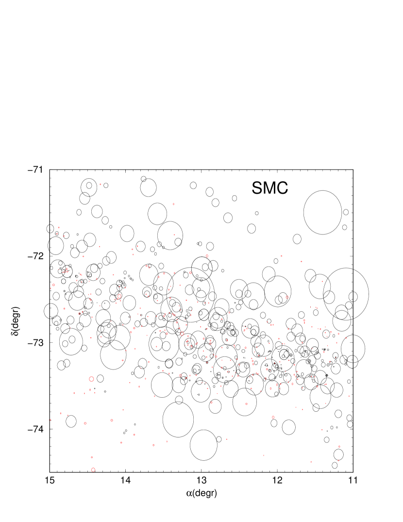
Figure 1: Top: LMC non-cluster (Table 1) structures are clumpier (left) than the clusters (right). Bottom: When cluster (red circles) and non-cluster (black) angular sizes are shown, hierarchical structuring appears to occur in these typical LMC (left) and SMC (right) fields. By far, most of the objects with a large angular size in the bottom panels are non-clusters

.

In a hierarchical scenario, the turbulent gas forms large-scale structures (clusters and loose groups) with a mass distribution following a power-law of negative slope, i.e. $dN/dM\propto M^{-\beta}$, with $\beta\approx 2$, consistent with the mass distribution functions measured in several galaxies (Elmegreen 2008).

Recent studies came up with robust evidence indicating that star-forming regions are indeed hierarchically structured, for instance in the nearby spiral galaxies M 33 (Bastian et al. 2007), M 51 (Bastian et al. 2005b), and NGC 628 (Elmegreen et al. 2006), the Local Group dwarf irregular galaxy NGC 6822 (Karampelas et al. 2009), the Galactic disk (de la Fuente Marcos & de la Fuente Marcos 2009), and the Gould Belt (Elias, Alfaro & Cabrera-Caño 2002).

Given the relative proximity, the Magellanic Clouds are an excellent environment to investigate the above issues. For instance, Efremov & Elmegreen (1998) found that the average age difference between pairs of LMC clusters increases as a function of their distance, which implies hierarchical star formation coupled to evolutionary effects. The angular correlation of LMC stellar populations for separations between 2′ ($\sim 30$ pc) and 40′ ($\sim 550$ pc) also implies large-scale hierarchical structure in current star formation (Harris & Zaritsky 1999). The character of the LMC HI structure as a function of scale, the filamentary and patchy structures of the high- and low-emission regions respectively, suggest that most of the ISM is fractal, presumably the result of pervasive turbulence, self-gravity, and self-similar stirring Elmegreen, Kim & Staveley-Smith 2001). More recently, Bastian et al. (2009) found a highly substructured and rapidly evolving distribution in the LMC stars. They suggest that all of the original structure is erased in $\sim 175$ Myr (approximately the LMC crossing time), with small-scale structures mixing first. Similar conclusions apply to the SMC, in which stars appear to have formed with a high degree of (fractal) sub-structure, possibly imprinted by the turbulent nature of the parent gas; these structures are subsequently erased by random motions in the galactic potential on a time-scale of a crossing time through the galaxy (Gieles, Bastian & Ercolano 2008).

In this paper we investigate the degree of spatial correlation among the different kinds of LMC and SMC extended structures listed in the updated catalogue of Bica et al. (2008), together with its relation to star formation. We also study properties of their size distribution functions. Only two wide-apart age ranges are used for spatial correlation purposes: (i) very young objects (not older than $\sim 20$ Myr, and probably younger than $\sim 10$ Myr), which encompass clusters related to nebular emission and associations related or not to emission, as classified and catalogued from sky survey plates by Bica et al. (2008) and references therein, and (ii) old clusters (older than $\sim 600$ Myr). According to our definition, the dynamical age of the very young clusters is lower (Sect. 5) than the crossing time (of the host galaxy), while for the old ones it corresponds to several crossing times, which is important for interpreting the spatial correlation in different time periods. Clusters within the wide age range $\approx 20-600$ Myr are not used in the spatial correlation analysis (Sect. 5).

Only the Magellanic Clouds have so far such a deep, homogeneous information on star clusters, associations and nebulae. Exceptions are some neighbouring dwarf galaxies that have been surveyed and are (i) featureless (Ursa Minor), (ii) contain a few globular clusters (Fornax) or, (iii) star-forming events like in the Clouds (e.g. NGC 6822 - Karampelas et al. 2009).

This paper is organised as follows. In Sect. 2 we briefly discuss the updated Magellanic System catalogue. In Sect. 3 we describe the selection criteria for star clusters older than the Hyades. In Sect. 4 we discuss the size (and mass, for star clusters) distribution functions of the different classes of objects. In Sect. 5 we examine the spatial correlation of the different structures by means of two-point correlation functions. Concluding remarks are given in Sect. 6.

2 The updated MC Catalogue

Properties of the updated MC catalogue are fully discussed in Bica et al. (2008). We recall here the basic statistical properties. Taking the LMC, SMC and the Bridge together, the updated catalogue contains, respectively, 3740 classical star clusters, 3326 associations, 1445 emission nebulae, and 794 HI shells and supershells. With the recent additions and cross-identifications, Bica et al. (2008) contains about 12% more objects than those in Bica et al. (1999) and Bica & Dutra (2000) together.

Table 1: LMC and LMC Extended Object Properties

		LMC			SMC			LMC$+$SMC
Class	Age	N	$R_{max}$	$\alpha$	N	$R_{max}$	$\alpha$	N	$R_{max}$	$\alpha$	Comments
	(Myr)		(pc)			(pc)			(pc)
C	Any	2268	38	$3.53\pm 0.22$	456	30	$3.01\pm 0.24$	2724	38	$3.60\pm 0.23$	Ordinary cluster
CN	$\la 10$	81	25	$3.85\pm 0.62$	9	8	$2.76\pm 0.58$	90	25	$3.73\pm 0.67$	Cluster in nebula
CA	$5-20$	738	21	$3.19\pm 0.59$	110	11	$2.59\pm 0.89$	848	21	$3.10\pm 0.57$	Cluster similar to assoc.
AC	$10-30$	1185	32	$4.42\pm 0.24$	60	14	$2.44\pm 0.17$	1245	32	$4.11\pm 0.21$	Assoc. similar to cluster
NC	$\la 5$	183	16	$3.52\pm 0.30$	72	8	$4.15\pm 0.66$	255	16	$3.62\pm 0.26$	Nebula w/prob. emb. cluster
Clusters		4455	38	$3.29\pm 0.22$	707	30	$3.04\pm 0.23$	5162	38	$3.20\pm 0.19$	C+CN+CA+NC+AC
A	$\la 30$	1476	171	$2.10\pm 0.15$	130	292	$2.23\pm 0.23$	1606	292	$2.21\pm 0.14$	Ordinary association
AN	$\la 10$	217	262	$1.80\pm 0.11$	39	62	$2.07\pm 0.30$	256	265	$1.70\pm 0.11$	Association w/nebular traces
NA	$\la 5$	817	472	$1.75\pm 0.06$	169	283	$2.08\pm 0.17$	986	472	$1.73\pm 0.07$	Nebula w/embedded assoc.
DAN${}^{\dagger}+$DNC†	$\la 5$	77	400	$1.15\pm 0.09$	33	144	$1.02\pm 0.16$	110	400	$1.05\pm 0.09$	Decoupled structures
Non-clusters		2587	472	$1.94\pm 0.06$	371	288	$2.04\pm 0.13$	2958	472	$1.89\pm 0.06$	A+AN+NA+DAN+DCN
SNR	—	52	78	$0.86\pm 0.10$	22	38	$0.50\pm 0.57$	74	78	$0.85\pm 0.13$	Supernova remnants
HI shells	—	124	472	$3.43\pm 0.40$	545	482	$2.88\pm 0.20$	794	477	$2.82\pm 0.05$	HI shells and supershells

• N is the number of objects; $\alpha$ is the power-law slope ($\phi(R)=dN/d\,R\propto R^{-\alpha}$) fitted to the large radii range (Sect. 4); $R_{max}$ is the maximum radius measured in each class. ($\dagger$) - small cluster or association in large nebula. DCN and DAN: the nebular and stellar component of the objects can be distinguished on Sky Survey plates.

Especially in view of the spatial correlation analysis (Sect. 5), in this paper we restrict the object selection to the LMC and SMC, not including Bridge or extended Wing structures. A census of the LMC and SMC extended structures is provided in Table 1, separated according to object class and including the probable age range. We note that, based on similarities observed in the size distributions (Sect. 4), in the present paper we include the AC and NC classes (relatively young objects) into the cluster classification, thus resulting in a higher number of such objects than quoted in Bica et al. (2008). Besides the latter two classes, the cluster classification also contains the C, CN and CA classes. As non-clusters (structures mostly associated with star formation environments) we take the A, AN, NA, DAN and DNC classes (see Table 1 notes). The SNR and HI shells are not used because they are object classes apart and their size distribution functions are significantly different from those of the clusters and non-clusters (Fig. 4).

Figure 1 (top panels) shows the angular distribution of the 4455 LMC clusters (left) and 2587 non-clusters (right). Both kinds of structures trace well-known LMC (and SMC) structures (e.g. Bica et al. 2008 and references therein). It is also clear that the non-clusters appear to present a high degree of spatial correlation, with most of them tightly clumped together. This applies as well to the clusters, but to a lesser degree, because young and old clusters present significantly different levels of spatial self-correlation, the latter being essentially non-correlated (Sect. 5).

When the angular sizes are considered (bottom panels), we see that most structures are arranged according to complex patterns, with sub-structures located inside larger ones.

3 Old star clusters

The identification, characterisation and spatial distribution of old star clusters in the Clouds has been a major concern throughout decades (e.g. Hodge 1960; Hodge 1982; Brück 1975; van den Bergh 1981; Bica et al. 1996). By old or red star clusters we mean those older than the Hyades ($\approx 630$ Myr), or intermediate age clusters (IACs) up to classical globular cluster ages. We adopted the definition of old star cluster by Janes & Phelps (1994) and Friel (1995). Magellanic Cloud clusters about this age appear to show dynamically evolved surface density profiles (e.g. Mackey & Gilmore 2003a; Mackey & Gilmore 2004; Carvalho et al. 2008). Since the cluster age distribution function drops significantly with age (see, e.g., Fig. 2 of de Grijs & Goodwin 2009 for the Magellanic Clouds), the presently adopted old cluster definition encompasses a statistically more significant sub-sample (Sect. 3.2) than what would result for, e.g. clusters older than 1 Gyr.

Clusters are expected to mix up by random motions under the galactic potential on a time-scale of a crossing time that, for the SMC, is of the order of 75 Myr (Gieles, Bastian & Ercolano 2008), and about twice that value for the LMC. Thus, the old clusters as defined above have ages that correspond to several crossing times of the respective galaxy, and any memory of the clumpy structures where they were born should have been erased. In this sense, they can be used as probes of the long-term behaviour of the cluster spatial correlation (Sect. 5).

3.1 Short cluster history in the Clouds: towards taking the census of the total population?

Kron (1956) and Lindsay 1958 discovered luminous and intermediate luminosity clusters in the SMC using plate material. Hodge & Wright (1974) and Brück (1975) discovered intermediate and low luminosity clusters, while Hodge (1986) discovered even fainter ones by means of 4m telescope plates. Bica & Schmitt (1995) discovered low luminosity clusters on sky survey plates, while Pietrzynski et al. (1998) discovered low luminosity clusters by means of CCD imaging.

Hodge (1960) identified 35 luminous old clusters by means of non-calibrated CMDs, of which 11 were discoveries. Shapley & Lindsay (1963) and Lyngå & Westerlund (1963) discovered most of the luminous and intermediate-luminosity clusters in the LMC, the latter work being dedicated to the outer parts. Hodge & Sexton (1966) discovered intermediate-luminosity clusters, while Hodge (1988) low-luminosity ones with 4m-telescope plates. Olszewski et al. (1988) discovered low-luminosity clusters in the outer parts. Kontizas et al. (1990) discovered additional intermediate and low-luminosity clusters, while Bica et al. (1999) discovered a large number of low luminosity clusters on sky survey plates. Pietrzynski et al. (1999) discovered low-luminosity clusters in the LMC with CCD observations.

Bica et al. (2008) and references therein have cross-identified these catalogues and a number of other studies, and is particularly suitable as a starting point for a deeper new survey such as the Visible and Infrared Survey Telescope for Astronomy (VISTA). It also provides a mean to properly acknowledge previous discoveries and to unambiguously establish new cluster findings.

Santiago et al. (1998) serendipitously detected two faint clusters in an LMC bar field using HST. The clusters have masses comparable to those of Galactic open clusters and ages in the range $200-500$ Myr. The clusters are extremely faint on DSS and XDSS images, which suggests that the Clouds might harbour an important open cluster counterpart population. Besides being a powerful tool to explore probable red brighter and intermediate-luminosity star clusters in the Clouds (Table 2), VISTA will be essential also to detect such a possible population of open cluster counterparts, and estimate their age distribution.

Based on the broad-band UBVR photometry of Hunter et al. (2003), de Grijs & Anders (2006) derived absolute values of age and mass for a sample of LMC star clusters to study the cluster formation rate, their characteristic disruption time-scale and the cluster mass function in different mass ranges. The same sample was used for further investigation of the cluster formation rate and the disruption time-scale by Parmentier & de Grijs (2008). The same method was applied to a sample of SMC clusters by de Grijs & Goodwin (2008) to study the infant mortality. Our approach in this paper differs in several ways, since we intend to build statistically significant samples of clusters (as well as associations and emission nebulae) characterised by very different age ranges.

3.2 Construction of the present sample of old clusters

We compiled ages from the literature later than 1988, as determined from CMDs. There are 85 and 202 old clusters with ages derived from CMDs for the SMC and LMC respectively, and they are provided in Table 2. Columns 1 to 8 of this table contain the same information as the general catalogue (Bica et al. 2008). We now introduced additional columns that provide the age determination method (Col. 9), $\log(Age)$ (Col. 10), and the relevant references for the age (Col. 11). Note that several references are compilations themselves, so more references are therein.

Table 2: Old SMC and LMC clusters inferred from different methods - Excerpt

Designations	$\alpha[J2000]$	$\delta[J2000]$	Class	a	b	PA	Classification	Method	log(Age)	Ref
	($hms$)	(°′″)		(′)	(′)	(°)			(yr)
(1)	(2)	(3)	(4)	(5)	(6)	(7)	(8)	(9)	(10)	(11)
SMC Star Clusters
AM-3,ESO28SC4	23:48:59	-72:56:43	C	0.90	0.90	-	Old IAC	CMD	9.74	R3
L1,ESO28SC8	0:03:54	-73:28:19	C	4.60	4.60	-	Globular Cluster	CMD	9.95	R12
”								CMD	9.88	R26
L2	0:12:55	-73:29:15	C	1.20	1.20	-		PLA	Red	R55
L3,ESO28SC13	0:18:25	-74:19:07	C	1.00	1.00	-		PLA	Red	R36
K1,L4,ESO28SC15	0:21:27	-73:44:55	C	2.20	2.20	-		CMD	9.49	R18
BOLOGNA A	0:21:31	-71:56:07	C	0.80	0.80	-	sup 47 Tucanae	CMD	IAC	R56
L5,ESO28SC16	0:22:40	-75:04:29	C	1.10	1.10	-	Old IAC	CMD	9.61	R18
LMC Star Clusters
NGC1466,SL1,LW1,ESO54SC16,KMHK1	3:44:33	-71:40:17	C	3.50	3.50	-	Globular Cluster	CMD	10.17	R41
SL2,LW2,KMHK2	4:24:09	-72:34:23	C	1.60	1.60	-		PLA	Red	R55
KMHK3	4:29:34	-68:21:22	C	0.80	0.80	-		PLA	Red	R55
NGC1629,SL3,LW3,ESO55SC24,KMHK4	4:29:36	-71:50:18	C	1.70	1.70	-		COL	Red	R5
HS8,KMHK5	4:30:39	-66:57:25	C	0.80	0.80	30		PLA	Red	R55
SL4,LW4,KMHK7	4:32:38	-72:20:27	C	1.70	1.70	-		CMD	9.23	R6
KMHK6	4:32:48	-71:27:30	C	0.60	0.55	80		PLA	Red	R55

• Cols. 5 and 6: semimajor axes $a$ and $b$; Col. 7: position angle; Col. 9: old age method. Col. 10: $\rm\log(Age)$ when available, or age class. References (Col. 11): R3: Da Costa (1999); R5: Bica et al. (1996); R6: Geisler et al. (1997) - relative ages; R12: Crowl et al. (2001); R18: Piatti et al. (2005); R26: Glatt et al. (2008); R36: Brück (1975), Brück (1976); R41: Piatti et al. (2009); R55: present paper - red (old) cluster by plate inspection; R56: Bellazzini, Pancino & Ferraro (2005).

We employed observed (Rafelski & Zaritsky 2005), reddening-corrected (Hunter et al. 2003) integrated colours, and SWB types to identify old clusters (typically SWB IVB or later, Bica et al. 1996), for clusters that still lack CMD ages. We also included results from integrated spectroscopy (Ahumada et al. 2002). By inspection of DSS and XDSS images we excluded clusters with apparent contamination by relatively bright stars, concerning integrated colours and spectra. We found 41 and 117 old clusters in the SMC and LMC respectively from integrated colours (Table 2).

Figure 2: Angular distribution of the LMC (left panels) and SMC (right) old star clusters with age obtained by means of CMDs, integrated colours and plate inspection.

Finally, following Brück (1975) and Brück (1976), we examined blue and red DSS and XDSS images, and ESO film sky survey plates to identify red clusters. It is remarkable how the red SMC clusters by Brück (1976) — his types T1 and T2 — have been confirmed as old clusters by means of deep CMDs. Brück disposed of U plates to help the classification. We dispose of blue and red plates, where it was basically possible to recognise clusters with brighter stars red from the RGB or bluer MS stars. Also, blue clusters have as rule more irregular angular distributions. Most clusters that we examined by this simple method are in the outer parts of the LMC. By means of integrated colours, Bica et al. (1996) found that the outer LMC disk appears to be essentially composed of old clusters. Our goal here is to provide a sample of probable red clusters suitable to correlation function tests, and to isolate that sample for CMD studies in view of VISTA and other large telescopes. There are 19 and 203 clusters, respectively in the SMC and LMC, that are probably old (red) from our plate inspections.

Table 2 also includes rather populous clusters that have CMDs, integrated colours or plate diagnostics pointing to a blue-red transition cluster, that occurs around 500 Myr. The sudden or perhaps rather smooth integrated colour change is expected from the so-called AGB and RGB phase transitions (e.g. Mucciarelli et al. 2006 and references therein). The present sample is a new one for such purposes. To minimise ambiguous age determinations, we have not included the blue-red transition clusters in our spatial correlation study, although they are, in principle, also old enough for dynamical purposes. Also, we note that Bica et al. (1996) decontaminated the clusters containing atypical bright stars superimposed. We examined all clusters showing red colours from Hunter et al. (2003) and Rafelski & Zaritsky (2005) on sky survey plates, and excluded those that appeared to be dominated by one or a few bright stars. We may have excluded some faint intrinsic old clusters with one or a couple bright AGB stars, but such stars are rare even in populous Magellanic Cloud clusters (e.g. Aaronson & Mould 1982).

In summary, there are 522 star clusters in the LMC that can be currently considered as old as, or older than the Hyades. The SMC contains 145 such cases. Considering the LMC and SMC together, the total sample of old/red clusters corresponds to a fraction of $\approx 13\%$ of the cluster-like structures (Table 2). Details on the angular distribution of this sub-sample are shown in Fig. 2. The old CMD sample shows a well-defined LMC bar, while The SMC probably shows a thick edge-on disk (Bica et al. 2008 and references therein). Red integrated colours complement these samples mostly for fainter clusters. The LMC plate sample corresponds essentially to the outer disk. We emphasise that the present sharp inner border of the old sample is an artifact, but not the outer ring structure, as can be seen in the most recent census of clusters and related objects (Bica et al. 2008). The outer LMC disk ring is a real feature, probably produced as a consequence of the last LMC/SMC encounter that took place $\approx 200$ Myr ago (Bekki & Chiba 2007). This structure is present in the uniform plate survey by Kontizas et al. (1990) and in that by Bica et al. (1999). The magnitude-limited integrated photometry of LMC clusters by Bica & Schmitt (1995) also showed this structure for the oldest age group. In the present study, essentially all known red clusters in the outer LMC are included in that locus. The geometries of the sub-samples were established by each survey, but have apparently not affected the correlation functions, as shown by the tests with different old cluster subsamples (Sect. 5).

In their surveys, Bica & Schmitt (1995), Bica et al. (1999), and Bica & Dutra (2000) employed film copies of the ESO Schmidt telescope Red Survey and the UK Schmidt telescope SERC-J (blue band) survey in Australia. The red plates trace emission nebulae by means of H$\alpha$. The limiting magnitudes are R=21.5 and Bj=22.5, respectively. Thus the detection limit of stars in clusters is very deep, especially in J. However, only the new generation of CCD surveys will permit to quantify the completeness of those samples compiled or discovered by our group, and certainly to explore an as yet undetected population of fainter objects.

4 Size distribution functions: structural hierarchy

The spatial distribution of interstellar gas follows a fractal structure ranging over many scales, from the subparsec at the smallest to the cluster and star complexes at the largest. This suggests that, if stars are formed mostly in the densest regions, they should also form in fractal patterns (e.g. Elmegreen & Elmegreen 2001 and references therein). Indeed, the power-law nature of the size distribution function has been observed in Galactic giant molecular clouds (Elmegreen & Falgarone 1996) and cloud clumps (Williams, Blitz & Stark 1995). The end result of this process is that the cluster size distribution should follow a declining power-law with size, a behaviour that has been observed in several galaxies (e.g. Elmegreen & Salzer 1999; Elmegreen et al. 2001; Bastian et al. 2005a).

Our first approach in the investigation of the hierarchical structures in the Clouds is by means of the size (i.e. absolute radius, $R_{\rm cl}$) distribution functions $\phi(\mbox{$R_{\rm cl}$})=dN/d\mbox{$R_{\rm cl}$}$. We build $\phi(\mbox{$R_{\rm cl}$})$ individually for all classes of objects listed in Table 1 based on the apparent major and minor axes given in the updated catalogue, together with the Cloud distances $d_{\rm LMC}\approx 50$ kpc and $d_{\rm SMC}\approx 60$ kpc (e.g. Schaefer 2008). Although the disks of both Clouds are inclined with respect to the line of sight, the effect of the distance correction on the absolute radius distribution is small, to within the error bars (see App. A).

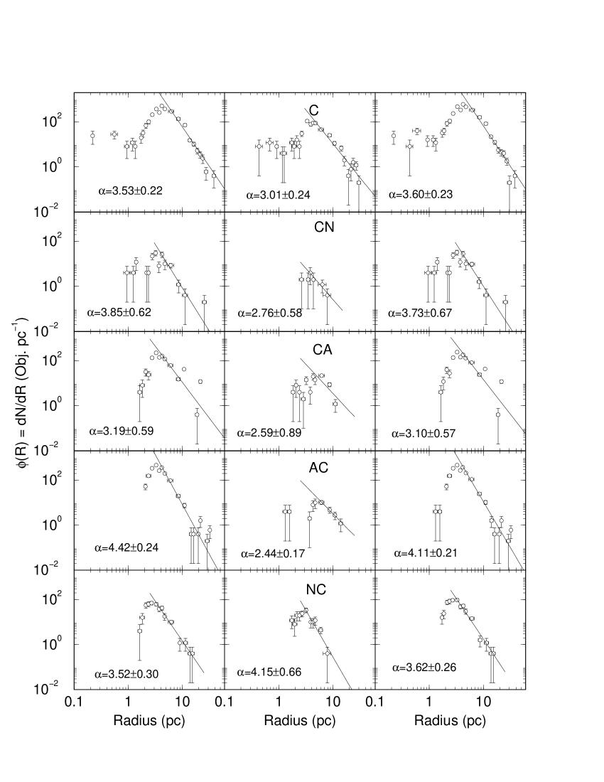
Figure 3: Radius distribution function of the cluster-like structures in the LMC (left panels), SMC (middle), and both Clouds combined (right). The radial range not affected by incompleteness is fitted with the power-law $\phi(R)\propto R^{-\alpha}$ (solid line).

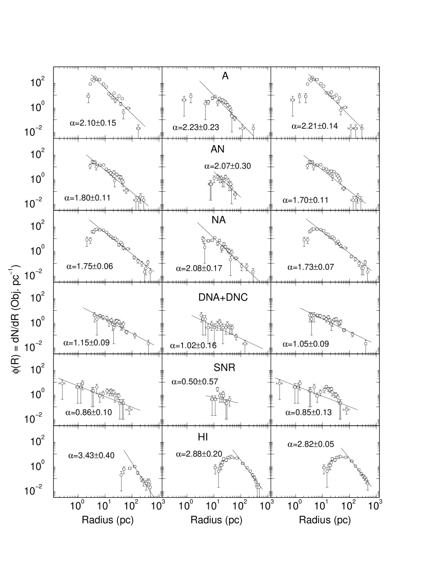
Figure 4: Same as Fig. 3 for the non-Cluster structures. Besides being structures apart, SNR and HI shells have distributions significantly different from those of the cluster-like and non-clusters.

The radius distribution functions for the cluster-like structures (Fig. 3) are characterised by a steep decline for $\mbox{$R_{\rm cl}$}\ga 4$ pc, which corresponds to about 0.25′. As we discuss in App. B, observational incompleteness probably accounts for the shape of $\phi(\mbox{$R_{\rm cl}$})$ in the small-size range, $\mbox{$R_{\rm cl}$}\la 4$ pc. The maximum radius ($R_{max}$) reached by the cluster-like structures in the LMC is $R_{max}\approx 40$ pc, and $R_{max}\approx 30$ pc in the SMC. Power-law fits ($\phi(\mbox{$R_{\rm cl}$})\propto\mbox{$R_{\rm cl}$}^{-\alpha}$) to the incompleteness-unaffected range are obtained with rather steep slopes, $\alpha\ga 3$, especially for the (statistically) well-defined distributions. The values of $R_{max}$ and $\alpha$ are given in Table 1.

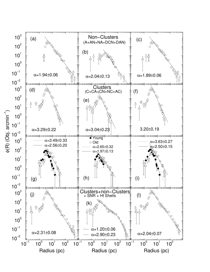
Figure 5: Same as Fig. 3 for the composite distribution functions of the non-clusters (panels a - c) and clusters (d - f). The sub-samples of the young and old clusters are in panels (g) - (i). All structures together, including SNR and HI shells, are shown in the bottom panels.

Figure 4 shows $\phi(\mbox{$R_{\rm cl}$})$ for the remaining object classes. Except for the SNR, the distributions are qualitatively similar to those in Fig. 3, with a decline for large radii. However, compared to the cluster-like classes, the power-law slopes are significantly shallower ($\alpha\la 2$) and the maximum radii are $\approx 10$ times as large, reaching $R_{max}\approx 500$ pc in the LMC and $R_{max}\approx 300$ pc in the SMC. The incompleteness-related turnover for the A, AN, and NA classes occurs at the same radii as that in the cluster-like objects. The HI shells, on the other hand, have a turnover at $\mbox{$R_{\rm cl}$}\approx 70$ pc ($\approx 4.4\arcmin$), which might reflect a real effect, not related to completeness.

Based on similarities of $R_{max}$ and $\alpha$, we define the C, CA, CN, NC, and AC classes as cluster-like structures, while A, AN, NA, DNC, and DAN as non-clusters. Their composite radius distributions are shown in Fig. 5, together with the power-law fit.

As expected from the above discussion, the cluster-like slopes for the LMC, SMC, and LMC$+$SMC distributions ($\alpha\approx 3$) are significantly steeper than the corresponding ones derived for the non-clusters ($\alpha\approx 2$). Figure 5 also shows the distributions obtained by adding all the structures, including the SNR and HI shells. While most of the individual features are preserved, the SMC profile, on the other hand, now requires two different power-laws to be described.

The slopes in the radius distribution of the non-clusters are consistent with those measured for H II regions in spiral galaxies (Oey et al. 2003).

4.1 Young and old clusters

We derive the size distribution functions of the young and old star cluster population. We take the CN (age $\la 10$ Myr) and NC (age $\la 5$ Myr) classes (Table 1) to represent the young star clusters. The old (age $\ga 600$ Myr) ones were selected according to the criteria discussed in Sect. 3.

Significant differences are observed in the size distribution functions (Figure 5), especially in the LMC. The distribution function of the young clusters falls off with radius at a steeper rate than the old ones, reaching a maximum size ($R_{max}\approx 15$ pc) less than half of that reached by the old ones ($R_{max}\approx 40$ pc). In the statistically more significant distributions of the LMC and SMC combined (right panels), the young clusters fall off with the slope $\alpha\approx 3.6$, while the old ones have $\alpha\approx 2.5$. The differences in $R_{max}$ and slope probably reflect the several $10^{8}$ yr of dynamical evolution of the old clusters, a consequence of which is an expansion of the outer parts (e.g. Khalisi, Amaro-Seoane & Spurzem 2007) of the clusters that survive the infant mortality (e.g. Goodwin & Bastian 2006) phase.

The size distribution functions of the young and old clusters fall off at a steeper rate ($\alpha>2$) than the non-clusters ($\alpha<2$).

4.2 A simple mass distribution function

Hierarchically structured gas is expected to form star clusters with mass distributed according to a power-law of the form $dN/d\mbox{$M_{\rm cl}$}\propto\mbox{$M_{\rm cl}$}^{-\beta}$, with $\beta\approx 2$ (e.g. Elmegreen 2008).

Below we apply a simple method to analytically transform the cluster radius distribution function into a mass distribution. We wish to test if our sample of LMC and SMC clusters basically follow the above mass distribution. We caution that our approach to the mass distribution is a simplification, since we do not take into account individual mass-to-light (M/L) ratios, which are known to vary considerably between young and old clusters (e.g. Bica, Arimoto & Alloin 1988; Charlot & Bruzual 1991; Leitherer et al. 1999). However, the presently extracted sample (Bica et al. 2008) is by far ($\approx 87\%$) dominated by young clusters and, thus, large variations of the M/L ratio are not expected. Besides, instead of computing individual masses from integrated luminosity, we use scaling relations that apply well to a wide variety (in terms of age, mass, and size) of Galactic star clusters to transform one kind of distribution function into another. In this sense, we expect that the adopted radius to mass transformation is representative of the average M/L ratio of the clusters.

We start by assuming a spherical star cluster with a mass radial density profile that can be described by a King-like function $\sigma_{M}(R)=\sigma_{M0}/(1+(R/R_{c})^{2})$, where $\sigma_{M0}$ is the surface mass density at the cluster centre and $R_{\rm c}$ is the core radius. We also consider that essentially all stars are contained within $0\leq R\leq\mbox{$R_{\rm cl}$}$, where $R_{\rm cl}$ is the cluster radius. The spatial mass density of such a structure can be computed from inversion of Abell’s integral,

$$\rho(R)=-\frac{1}{\pi}\int_{R}^{\infty}\frac{\partial\sigma_{M}(\chi)}{\partial\chi}\frac{d\chi}{\sqrt{\chi^{2}-R^{2}}}=\frac{\sigma_{M0}}{2\mbox{$R_{\rm c}$}}\left[\frac{1}{1+(R/\mbox{$R_{\rm c}$})^{2}}\right]^{3/2}.$$

Thus, the cluster mass can be computed from

$$\mbox{$M_{\rm cl}$}\approx\int_{0}^{\mbox{$R_{\rm cl}$}}\rho(R)4\pi\,R^{2}\,dR=2\pi\sigma_{M0}\mbox{$R_{\rm c}$}^{2}\times$$

$$~{}~{}~{}~{}~{}~{}~{}~{}~{}~{}~{}~{}~{}~{}~{}\times\left[arcsinh(\mbox{$R_{\rm cl}$}/\mbox{$R_{\rm c}$})-\frac{1}{1+(\mbox{$R_{\rm c}$}/\mbox{$R_{\rm cl}$})^{2}}\right].$$

Galactic star clusters with ages from a few Myr to $\sim 1$ Gyr, masses within $50\,\mbox{$M_{\odot}$}\la\mbox{$M_{\rm cl}$}\la 7\times 10^{3}\,\mbox{$M_{\odot}$}$, and radii within $\rm 2\,pc\la\mbox{$R_{\rm cl}$}\la 20$ pc, have the relation between $R_{\rm cl}$ and $R_{\rm c}$ well approximated by $\mbox{$R_{\rm cl}$}\approx 9\mbox{$R_{\rm c}$}$ (e.g. Bonatto & Bica 2009a). Comparable ratios are observed in LMC and SMC star clusters (e.g. Mackey & Gilmore 2003a; Mackey & Gilmore 2003b; Carvalho et al. 2008). Under these assumptions we have $\mbox{$M_{\rm cl}$}\approx 4\pi\sigma_{M0}\mbox{$R_{\rm c}$}^{2}\approx 0.16\,\sigma_{M0}\mbox{$R_{\rm cl}$}^{2}$. This equation, together with central mass densities in the range $30\mbox{$M_{\odot}$}\,pc^{-2}\la\sigma_{M0}\la 600\mbox{$M_{\odot}$}\,pc^{-2}$, accounts for the distribution of cluster mass and core radius (Bonatto & Bica 2009b). Then, the transformation of the radius distribution to mass is given by $\phi(\mbox{$M_{\rm cl}$})=\phi(\mbox{$R_{\rm cl}$})/(0.31\sigma_{M0}\mbox{$R_{\rm cl}$})$, and the average cluster mass-density is a declining function of the cluster radius, $\bar{\rho}(\mbox{$M_{\odot}$}\,pc^{-3})=\frac{\mbox{$M_{\rm cl}$}}{(4/3)\pi\mbox{$R_{\rm cl}$}^{3}}\approx\frac{\sigma_{M0}}{27}\mbox{$R_{\rm cl}$}^{-1}$. For a given $R_{\rm cl}$, the radius to mass scalings depend only on $\sigma_{M0}$ as $\mbox{$M_{\rm cl}$}\propto\sigma_{M0}$ and $\phi(\mbox{$M_{\rm cl}$})\propto\sigma_{M0}^{-1}$ that, for different values of $\sigma_{M0}$, preserve the shape of the mass distribution, only changing the mass values.

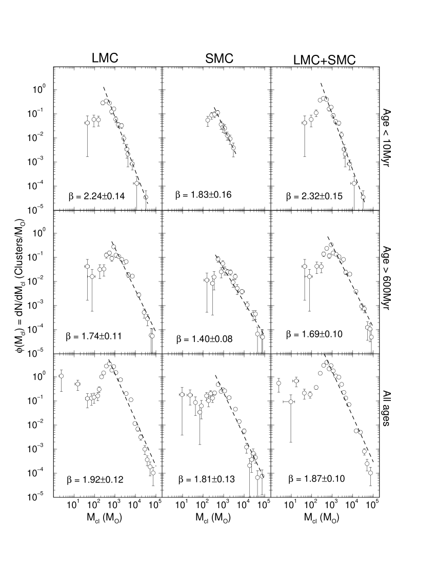
Figure 6: Estimated mass distribution functions with a power-law ($\phi(\mbox{$M_{\rm cl}$})\propto\mbox{$M_{\rm cl}$}^{-\beta}$) fitted to the large cluster mass range of the LMC (left panels), SMC (middle), and the combined LMC$+$SMC (right) clusters. Age ranges are $\la 10$ Myr (top panels), $\ga 600$ Myr (middle), and all ages (bottom).

We use the above scaling relations to transform the cluster radius distribution functions (Fig. 5) into mass distributions, $\phi(\mbox{$M_{\rm cl}$})d\mbox{$M_{\rm cl}$}=\phi(\mbox{$R_{\rm cl}$})d\mbox{$R_{\rm cl}$}$, separately for the LMC and SMC, and the combination of both, LMC$+$SMC. We also consider the age ranges $\la 10$ Myr, $\ga 600$ Myr, and clusters of all ages combined. The average value (Galactic star clusters - Bonatto & Bica 2009b) of the central mass density, $\sigma_{M0}\approx 300\mbox{$M_{\odot}$}\,pc^{-2}$, is used to compute the mass distributions (Fig. 6); fit parameters are given in Table 3. The mass distribution of the very young clusters in both Clouds falls off at a steeper rate towards large masses than that of the old ones, which is consistent with a mass-dependent disruption time-scale (e.g. Lamers et al. 2005). Also, the slopes are steeper in the LMC than in the SMC. These slopes are consistent with those of the mass distributions of star clusters in different galaxies (Elmegreen 2008).

Table 3: Mass distribution properties

LMC

SMC

LMC$+$SMC

Age range

N

$M_{min}$

$M_{max}$

$\beta$

N

$M_{min}$

$M_{max}$

$\beta$

N

$M_{min}$

$M_{max}$

$\beta$

(Myr)

($M_{\odot}$)

($M_{\odot}$)

($M_{\odot}$)

($M_{\odot}$)

($M_{\odot}$)

($M_{\odot}$)

$\la 10$

201

$5.0\times 10^{2}$

$3.2\times 10^{4}$

$2.24\pm 0.14$

47

$5.0\times 10^{2}$

$3.0\times 10^{3}$

$1.83\pm 0.16$

198

$5.0\times 10^{2}$

$3.2\times 10^{4}$

$2.32\pm 0.15$

$\ga 600$

435

$9.0\times 10^{2}$

$7.0\times 10^{4}$

$1.74\pm 0.11$

135

$5.0\times 10^{2}$

$8.0\times 10^{4}$

$1.40\pm 0.08$

552

$9.0\times 10^{2}$

$8.0\times 10^{4}$

$1.69\pm 0.10$

All ages

3700

$5.0\times 10^{2}$

$7.0\times 10^{4}$

$1.92\pm 0.12$

629

$5.0\times 10^{2}$

$8.0\times 10^{4}$

$1.81\pm 0.13$

4271

$5.0\times 10^{2}$

$8.0\times 10^{4}$

$1.87\pm 0.10$

• N is the number of clusters used to fit the mass range $M_{min}<\mbox{$M_{\rm cl}$}<M_{max}$ with the power-law $\phi(\mbox{$M_{\rm cl}$})\propto\mbox{$M_{\rm cl}$}^{-\beta}$. $M_{min}$ and $M_{max}$ computed for $\sigma_{M0}=300\mbox{$M_{\odot}$}\,pc^{-2}$; they scale linearly with $\sigma_{M0}$.

The mass distributions of the very young clusters are characterised by a maximum mass of $M_{max}\approx 1.2\times 10^{4}\,\mbox{$M_{\odot}$}$ (LMC) and $M_{max}\approx 3\times 10^{3}\,\mbox{$M_{\odot}$}$ (SMC), while for the old ones it is $M_{max}\approx(7-8)\times 10^{4}\,\mbox{$M_{\odot}$}$ in both Clouds. The latter values are considerably higher than the maximum mass of typical Galactic open clusters (e.g. Piskunov et al. 2007). The decline in the number of clusters with mass below $M_{min}$ (Table 3) is probably related to observational incompleteness in the detection of small clusters (Sect. 4). For comparison purposes we also show in Fig. 6 the mass distributions for the LMC$+$SMC clusters, as well as those corresponding to clusters of all ages, in which the basic features of the individual distributions are preserved.

Interestingly, the maximum mass of the LMC clusters younger than $\approx 30$ Myr (de Grijs & Anders 2006), and SMC ones younger than $\approx 10$ Myr (de Grijs & Goodwin 2008), is about 2.4 times higher than that of the very young LMC and SMC clusters (Table 3). For LMC clusters younger than $\approx 5.6$ Gyr (de Grijs & Anders 2006) and SMC ones younger than $\approx 1$ Gyr (de Grijs & Goodwin 2008), the ratio increases to $\approx 4$. Although the somewhat different age ranges, consistency between both sets of $M_{max}$ values can be reached with the central mass densities $\sigma_{M0}\approx 700\mbox{$M_{\odot}$}\,pc^{-2}$ and $\sigma_{M0}\approx 1200\mbox{$M_{\odot}$}\,pc^{-2}$, respectively for the very young and old clusters. The somewhat higher values of $\sigma_{M0}$ in the MCs clusters, with respect to the Galactic open clusters, is consistent with the relative cluster mass ranges encompassed by the LMC (de Grijs & Anders 2006), SMC (de Grijs & Goodwin 2008), and Milky Way (Piskunov et al. 2007) mass distributions.

Finally, if we take into account variations of M/L with age for the dominant (in number) young clusters (e.g. Bruzual & Charlot 2003), the actual mass values for clusters younger than $\approx 8$ Myr would be $\ga 30\%$ lower than the average-(M/L) estimates above, and $\approx 20-40\%$ higher for those with age within $\approx 13-30$ Myr. Given that the number of clusters decreases with age (see, e.g. de Grijs & Goodwin 2009, for the age-distribution of the MC clusters), our mass estimates in each bin of the mass distributions (Fig. 6) may be somewhat overestimated.

5 Hierarchy associated with star formation

In a hierarchical scenario, young star clusters are expected to preserve some memory of the physical conditions prevailing in their birthplace. Because of random motions along many orbits under the galactic potential, the spatial distribution of old star clusters, on the other hand, should be very little reminiscent of the primordial one. According to this scenario, the frequency of young star clusters lying relatively close to each other - and to star-forming structures - should be higher than for the old ones. Based on the 590 LMC clusters ($\approx 13\%$ of the present sample size - Table 1) catalogued by Bica et al. (1996) with ages derived from the UBV colours by Girardi et al. (1995), Efremov & Elmegreen (1998) found that the average age difference between pairs of clusters increases with the separation, which they interpreted as resulting from star formation that is hierarchical in space and time. A similar result - and interpretation - was found by de la Fuente Marcos & de la Fuente Marcos (2009) for pairs of open clusters in the Milky Way disk.

We investigate this point further by means of the degree of spatial correlation among groups of objects characterised by different age ranges and sizes. We use the young and old star clusters defined in Sect. 4.1.

Consider two groups of objects, $A$ and $B$. For each object in $A$, we compute the angular separation with respect to all objects in $B$. After applying the same procedure to all objects in $A$, we build the two-point-correlation function (2PCF), which measures the fractional number of pairs $N$ that lie within a given separation $\xi$ and $\xi+d\xi$, $2PCF(\xi)\equiv dN/d\xi$. According to this definition, the 2PCF is simply the angular separation distribution function.

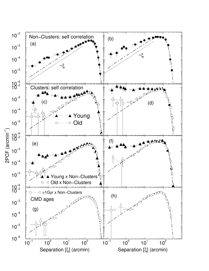
Figure 7: Two-point correlation functions for the LMC (left panels) and SMC (right) extended objects. The simulated 2PCF (dot-dashed line) increases linearly with the separation $\xi$. Panels (a) - (d): spatial self-correlation for the non-clusters and clusters. Panels (e) - (f): degree of spatial correlation of the young and old (older than the Hyades) clusters with the non-clusters. Panels (g) - (h): same as above for the clusters older than 1 Gyr, with the age determined from CMDs.

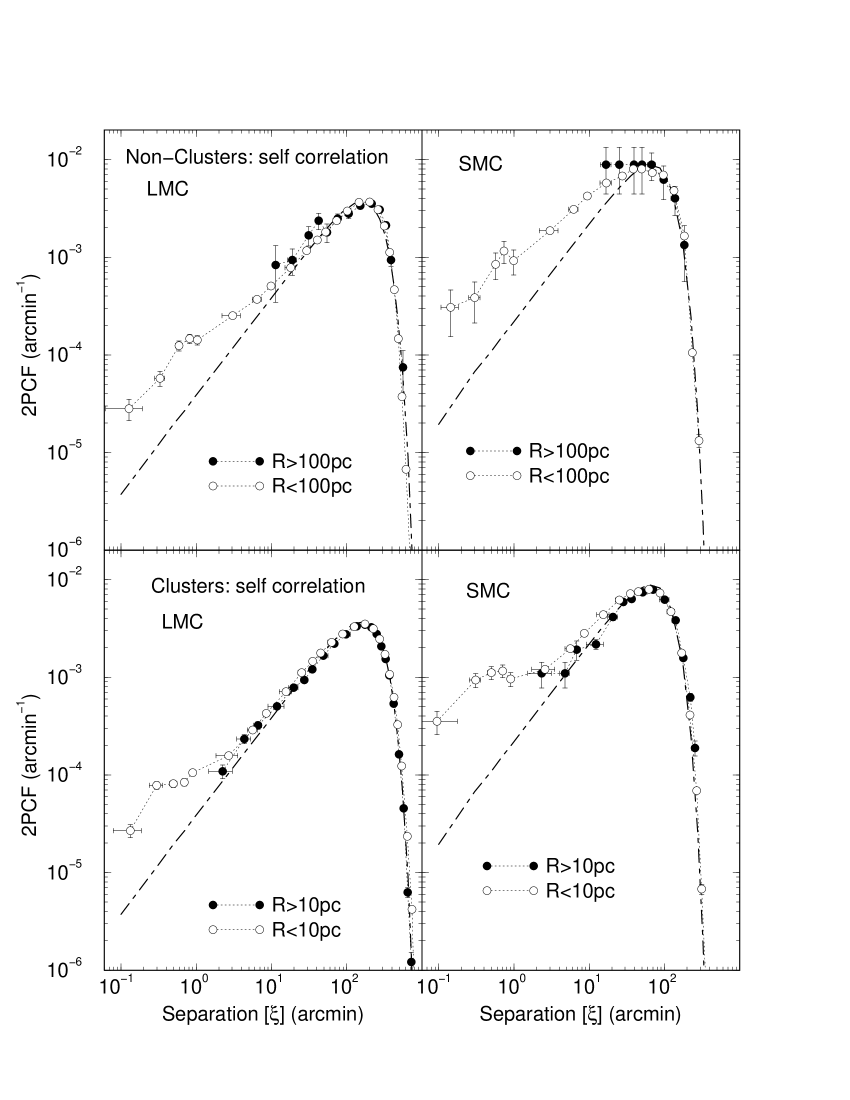
Figure 8: Same as Fig. 7 for the composite distribution functions of the non-clusters (top panels) and clusters (bottom), but differentiating for object size ($R$).

Artificial 2PCFs built with samples of points that emulate both the geometry and object distribution of the LMC and SMC are used to check the statistical significance of the spatial correlations. In the simulations we randomly select the right ascension ($\alpha$) and declination ($\delta$)coordinates of a given point within the actual ranges spanned by each Cloud (Fig. 1) and with the same number-frequency as the observed ones.

Irrespective of the adopted geometry, a random distribution of objects would produce a number of neighbours within a given separation $\xi$ that increases as $N(\xi)\propto\xi^{2}$, at least for a maximum separation $\xi_{max}$ (which should scale with the angular size of the simulated field). Thus, the 2PCFs should increase with $\xi$ as $dN/d\xi\propto\xi$. Indeed, the 2PCFs derived with the simulations (Fig. 7) present the expected dependence with separation for $\xi_{max}\la 80\arcmin\approx 1200$ (LMC) and $\xi_{max}\la 40\arcmin\approx 700$ pc (SMC). Beyond these values both the measured and simulated 2PCFS consistently drop, as a consequence of the limited size of the Clouds.

As a first step we compute the spatial self-correlation functions, in which $A=B$, for the LMC and SMC (Fig. 7). Compared to the simulated 2PCFs, the non-clusters (top panels) present a relatively high degree of spatial self-correlation for separations smaller than $\xi\la 15\arcmin\approx 220$ pc (LMC) and $\xi\la 25\arcmin\approx 440$ pc (SMC). Young (age $\la 10$ Myr) clusters present a high degree of spatial self-correlation, from small to large scales (middle panels), $\xi\la 35\arcmin\approx 500$ pc (LMC) and $\xi\la 25\arcmin\approx 440$ pc (SMC). Old (age $\ga 600$ Myr) clusters, on the other hand, have a very low degree of spatial self-correlation, restricted to separations $\xi\la 0.6\arcmin\approx 9$ pc (LMC) and $\xi\la 1.7\arcmin\approx 30$ pc (SMC). Interestingly, the same pattern is obtained with the 2PCFs computed for the clusters older than 1 Gyr, with the age determined from CMDs. Some degree of spatial correlation at small separations among old clusters is expected, since the Clouds contain binary and/or merger star clusters preferentially of comparable ages (e.g. Bica et al. 1999; Dieball, Müller & Grebel 2002; Carvalho et al. 2008). In summary, young clusters have a probability of being clustered together significantly higher than old ones, both in the LMC and SMC. The dynamical age of clusters older than $600$ Myr corresponds to $\ga 4$ crossing times in the LMC, and $\ga 8$ in the SMC, while for the young ones (age $\la 10$ Myr) it is $\la 0.07$ and $\la 0.13$, respectively for the LMC and SMC. Given that a single crossing time is necessary to smear out most of the primordial structural pattern (Gieles, Bastian & Ercolano 2008), the above conclusion is consistent with the old clusters having been mixed up by the random motions under the galactic potential along several $10^{8}$ years, while the young ones still trace most of the birthplace pattern.

Now we test the degree of spatial correlation of the young and old clusters with the non-clusters (star-formation environments). As expected from the self-correlation analysis, the young clusters are highly correlated with the non-clusters (bottom panels). The old clusters, on the other hand, appear to have some spatial correlation with the non-clusters only at the very-small scales, $\xi\la 0.2\arcmin\approx 3$ pc (LMC) and $\xi\la 0.4\arcmin\approx 7$ pc (SMC). Part of this correlation may be due to projection effects on the bar. For larger separations the 2PCFs can be accounted for by the random distribution of objects.

5.1 Self-correlation and object size

Now we examine the spatial self-correlation among clusters and non-clusters of different radius ranges. Based on the respective radius distribution functions (Fig. 5), we take $R=10$ pc as the boundary between small and large clusters; for the non-clusters we take the boundary at $R=100$ pc. The derived correlation functions (Fig. 8) indicate that the small clusters are more spatially correlated than their large counterparts. The same applies to the non-clusters.

Again, this picture is what should be expected from a hierarchical structure.

5.2 Effective separation

Finally, we investigate the effective separation of the young and old clusters with respect to the non-clusters. We first compute the effective separation ($\xi_{eff}$) between a cluster and a non-cluster, which we define as the ratio of the angular distance ($\xi$, converted to the absolute scale) to the radius of the non-cluster ($R_{NC}$), $\xi_{eff}\equiv\xi/R_{NC}$. In this way, a cluster that is located inside a non-cluster has $\xi_{eff}<1$.

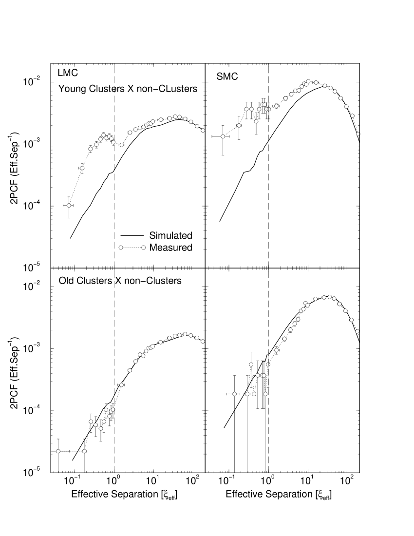
Figure 9: Two-point correlation functions of the effective separations ($\xi_{eff}\equiv\xi/R_{NC}$) between the young (top panels) and old (bottom) clusters with respect to the non-clusters, for the LMC (left panels) and SMC (right). Simulated 2PCFs are also shown (heavy-solid line). $\xi_{eff}=1$ is indicated by the dashed line.

Two-point correlation functions built with all the $\xi_{eff}$ between samples $A$ and $B$ thus provide a measure of the clustering among objects in both samples. For comparison we use simulated 2PCFs built for object samples (young and old clusters and non-clusters) with coordinates selected as described in Sect. 5. We now also include absolute radii separately for each sample, randomly taken from the observed distributions (Fig. 5).

The resulting 2PCFs are shown in Fig. 9. Consistently with the analyses of the previous sections, young clusters in both Clouds present a high degree of clustering with the non-clusters, especially for small effective separations ($\xi_{eff}<1$), but reaching as well high values of $\xi_{eff}$. In all scales, the clustering degree of the old clusters with respect to the non-clusters, on the other hand, can be accounted for by a random distribution of old clusters.

The above results are consistent with a strong hierarchical structuring of the young star clusters in both Clouds, including their time evolution effects.

6 Summary and conclusions

In broad lines, when star formation occurs in turbulent gas, large-scale structures are expected to be produced following a power-law mass distribution ($dN/dM\propto M^{-2}$ - Elmegreen 2008), and with hierarchically clustered young stellar groupings (e.g. Efremov 1995; Elmegreen 2006).

In the present paper we address the above issue by investigating the degree of spatial correlation among sets of LMC and SMC extended structures, characterised by different properties, and its relation to star formation. Based on the catalogue of Bica et al. (2008), we built sub-samples that basically contain star clusters (young and old) and nebular complexes (and their stellar associations). The latter structures are related to star-forming regions; for simplicity, we refer to them as non-clusters.

In all cases (Figs. 3-5), the radius distribution functions follow a power-law ($dN/dR\propto R^{-\alpha}$) decline for large radii with slopes that depend on object class (and age). Taking both Clouds combined, the non-clusters fall-off with a slope $\alpha\approx 1.9$ and reach sizes of $R_{max}\la 472$ pc. Old (age $\ga 600$ Myr) clusters present the somewhat steeper slope $\alpha\approx 2.5$, while the young (age $\la 10$ Myr) ones have the steepest slope $\alpha\approx 3.6$. The maximum size reached by clusters is less than $\approx 10\%$ of the non-clusters, with the old ones reaching a size $\approx 3\times$ bigger than the young ones. The differences in slope and maximum size between the young and old clusters can be accounted for by long-term dynamical effects acting on the clusters. By means of a radius to mass scaling (Sect. 4.2), we show that the mass distribution of the LMC and SMC clusters follows $dN/d\mbox{$M_{\rm cl}$}\propto\mbox{$M_{\rm cl}$}^{-\beta}$ (Fig. 6), with $\beta\approx 2$. Within the uncertainties (Table 3), this value agrees with the slope expected in a hierarchical scenario (Elmegreen 2008). Also, the mass distribution for clusters younger than $\approx 10$ Myr falls off towards large masses faster than the clusters older than $\approx 600$ Myr.

According to the two-point correlation functions (Sect. 5), the LMC and SMC star clusters younger than $\approx 10$ Myr present a very high degree of spatial correlation among themselves and, especially, with the non-clusters (Fig. 7). Clusters older than the Hyades ($\ga 600$ Myr) on the other hand, appear to have been heavily mixed up, probably because their ages correspond to several galactic crossing times and the strong perturbations associated with the LMC and SMC encounters (e.g. Bekki & Chiba 2007). When the analysis is restricted to clusters older than 1 Gyr - with the age determined from CMDs, the same conclusions are obtained.

Considering two different radius ranges, we show that small clusters ($R<10$ pc) and non-clusters ($R<100$ pc) are spatially self-correlated, while the large ones are not (Fig. 8). Also, young clusters in both Clouds present a very high degree of spatial clustering with the non-clusters, which does not occur with the old ones (Fig. 9).

The above results, expressed in terms of the spatial and size distribution of extended structures in the LMC and SMC, are fully consistent with a hierarchical star-formation scenario, in which star complexes are part of a continuous star-formation hierarchy that follows the gas distribution. Similar conclusions drawn from different methods and samples of objects have been obtained for the LMC (e.g. Elmegreen & Efremov 1996; Efremov & Elmegreen 1998; Harris & Zaritsky 1999; Livanou et al. 2006) and the SMC (e.g. Livanou et al. 2007; Gieles, Bastian & Ercolano 2008).

VISTA and other large telescopes will certainly uncover a large number of faint clusters in the Magellanic Clouds, with masses comparable to the Galactic open clusters. The same for embedded clusters. CMDs will provide accurate ages for them, as well as for many luminous, intermediate-luminosity, and low-luminosity clusters already catalogued. Also in this context, the catalogue by Bica et al. (2008) will be an essential tool, for having gathered and cross-identified the small and large structures in the Magellanic Clouds. The catalogue is also useful to help establish discoveries. The present work has provided as well a sub-catalogue of old and probable-old clusters, which can be useful also for VISTA studies.

Appendix A Disk inclination

The LMC and SMC disks are inclined with respect to the line of sight, and this should introduce some variations in the absolute sizes across the disks, as compared to the no-inclination approach adopted in Sect. 4.

To investigate the inclination effect on the radius distribution functions we assume $42\degr$ (e.g. Kontizas et al. 1990) and $40\degr$ (e.g. Stanimirović, Staveley-Smith & Jones 2004) as the inclination of the LMC and SMC disks with respect to the line of sight. Then, the absolute size of each cluster was recomputed for its corrected distance. The inclination-corrected radius distribution function (for the combined LMC$+$SMC clusters) is shown in Fig. 10, in which the un-corrected distribution (Fig. 5, panel f) is also shown for comparison purposes. We conclude that differences are small, essentially within the error bars. This can be accounted for by the relatively small distance corrections (with respect to the adopted Cloud distances), and that corrections affect objects both in the near and far sides in the opposite sense. On average, when a large number of objects is considered, the near and far-side corrections tend to self-compensate.

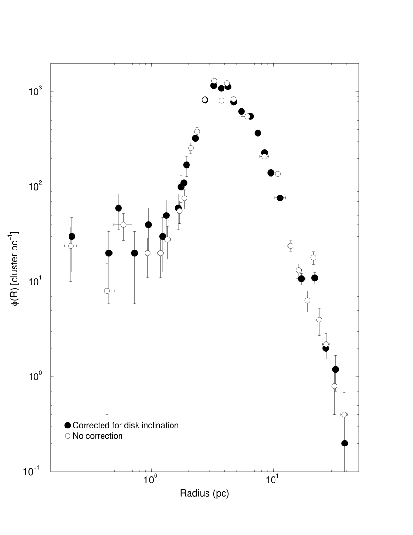
Figure 10: The inclination-corrected radius distribution function (filled symbols) is very similar to the uncorrected one (empty symbols).

Another effect that might introduce variations on absolute cluster size is the triaxial nature of the Clouds. The SMC, for instance, may have a line-of-sight depth of 6 - 12 kpc (e.g. Crowl et al. 2001). Thus, depth corrections would be of the same order as those related to inclination.

Appendix B Surface brightness incompleteness effects

Since extended structures are the focus of this work, the surface brightness (SB) incompleteness - which is expected to affect the radius distribution functions - should be taken into account. Basically, for a given luminosity, a more extended object will have on average a lower SB, and thus may not be detected by depth-limited surveys.

We examine this effect by means of a sample of $10^{7}$ artificial star clusters whose luminosity and radius distributions are described by $\phi(L)\,dL\propto L^{-2}\,dL$ and $\phi(R)\,dR\propto R^{-3.3}\,dR$, respectively. As discussed in Elmegreen & Elmegreen (2001), these analytical functions describe star clusters and H II regions. To reproduce the input radius and luminosity distributions, the simulated radius and luminosity are computed from $R=R_{m}/\left[1+n_{1}\left((R_{m}/R_{M})^{2.3}-1\right)\right]^{1/2.3}$ and $L=L_{m}/\left[1+n_{2}(L_{m}/L_{M}-1)\right]$, where $R_{m}$, $R_{M}$, $L_{m}$, and $L_{M}$ are the minimum and maximum radii and luminosities, and $n_{1}$ and $n_{2}$ are random numbers in the range $[0.0,1.0]$. The radius and luminosity of a given cluster are independently assigned. This process allows that clusters of the same size (and mass) - but different ages - may have different luminosities, as expected from the fading lines associated with the stellar evolution. Also, clusters with any radius within ($R_{m},R_{M}$) are allowed to have any luminosity within ($L_{m},L_{M}$). Then, the SB is computed in the usual way, $\mu=-2.5\log(L/\pi\,R^{2})+cnt$, in arbitrary units.

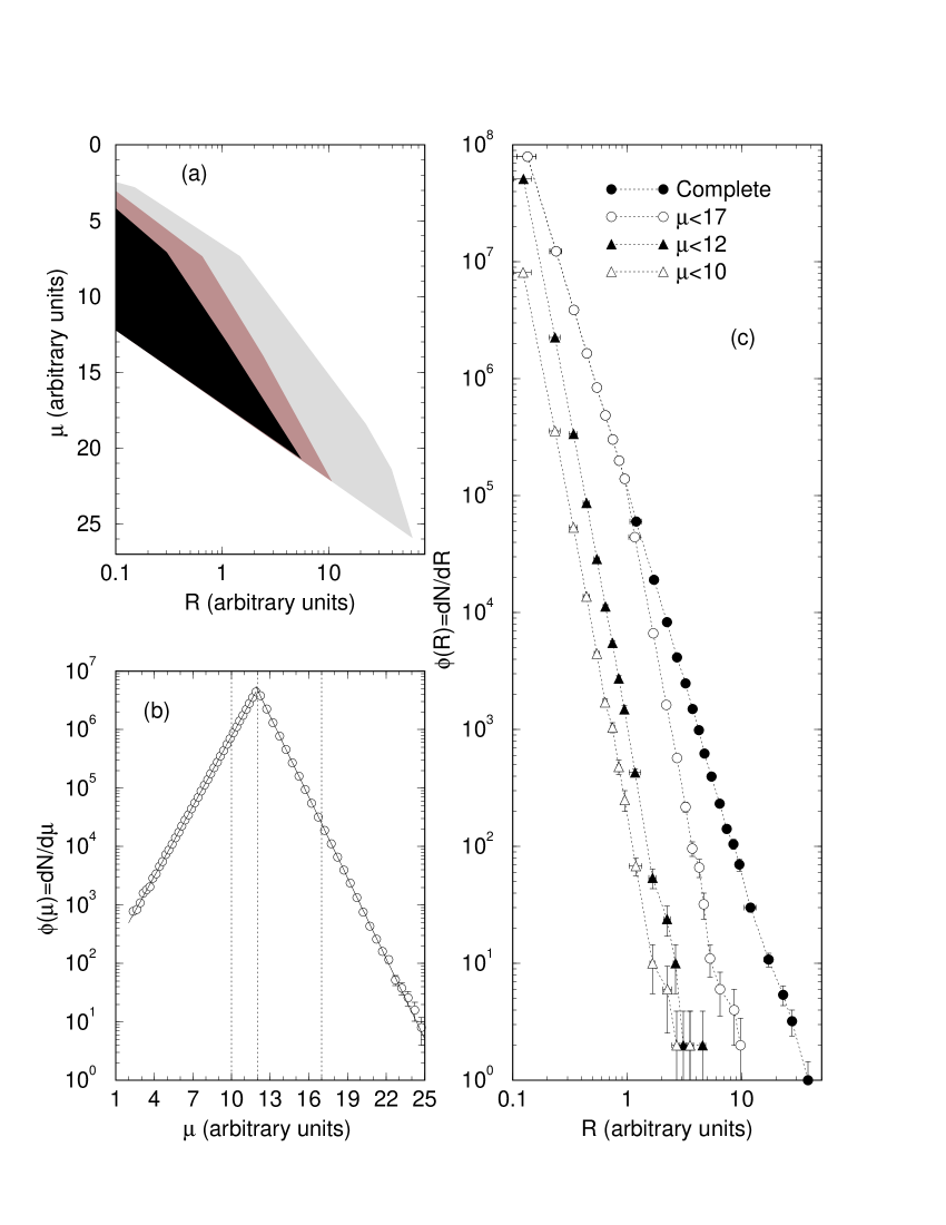
Figure 11: Panel (a): model SB distribution with respect to cluster radius; the density of points (number of simulated clusters) roughly increases towards heavier shades of gray. (b): SB distribution function (fitted with exponentials - solid line) showing the arbitrary thresholds (dashed lines). (c): radius distributions corresponding to the SB cuts in (b).

The results are summarised in Fig. 11. In general, the SB distribution among the simulated clusters agrees with the expected relation of decreasing SB with cluster radius (panel a). The two power-laws that describe the radius and luminosity distributions are reflected on the shape of the SB distribution (panel b), which first (beginning at the smallest and most luminous clusters) increases exponentially towards lower SBs, reaches a maximum, and falls off exponentially towards the largest and less luminous clusters. Based on this distribution we arbitrarily apply cuts for clusters with $\mu<17,~{}12,$ and $10$ and compute the corresponding radius distributions (panel c). Clearly, the SB cuts preserve the power-law character of the radius distribution. The major effect is a steepening of the slope. Indeed,while the complete radius distribution is a power-law of slope $\alpha=-3.3$, the SB-restricted distributions have $\alpha=-3.6\pm 0.1,~{}-5.0\pm 0.1$, and $\alpha=-5.2\pm 0.1$, respectively for $\mu<17,~{}12,$ and $10$.

In summary, SB-related incompleteness affects the radius distributions preferentially at the large-clusters tail, having little effect on the small clusters. Also, it preserves the power-law character of the radius distribution and, due to the preferential effect on large clusters, it produces a steepening of the distributions. Thus, the decrease in the observed radius distributions towards small clusters (Figs. 3 - 5) cannot be accounted for by SB incompleteness, and appears to be linked to an observational effect. In this sense, VISTA will be important also to explore the structure of small clusters in the Clouds, and to investigate the shape of the radius distribution at the small scales.

References

- Aaronson & Mould (1982) Aaronson M. & Mould J. 1982, ApJS, 48, 161
- Ahumada et al. (2002) Ahumada A.V., Clariá J.J., Bica E. & Dutra C.M. 2002, A&A, 393, 855
- Balbinot et al. (2009) Balbinot E., Santiago B.X., Bica E. & Bonatto C. 2009, MNRAS, 396, 1596
- Bastian et al. (2005a) Bastian N., Gieles M., Lamers H.J.G.L.M., Scheepmaker R.A. & de Grijs R. 2005a, A&A, 431, 905
- Bastian et al. (2005b) Bastian N., Gieles M., Efremov Yu. & Lamers H.J.G.L.M. 2005b, A&A, 443, 79
- Bastian et al. (2007) Bastian N., Ercolano B., Gieles M., Rosolowsky E., Scheepmaker R.A., Gutermuth R. & Efremov Yu. 2007, MNRAS, 379, 1302
- Bastian et al. (2009) Bastian N., Gieles M., Ercolano B. & Gutermuth R. 2009, MNRAS, 392, 868
- Bate (2009) Bate M.R. 2009, MNRAS, 392, 1363
- Bekki & Chiba (2007) Bekki K. & Chiba M. 2007, PASA, 24, 21
- Bellazzini, Pancino & Ferraro (2005) Bellazzini M., Pancino E. & Ferraro F.R. 2005, A&A, 435, 871
- van den Bergh (1981) van den Bergh S. 1981, A&AS, 46, 79
- Bica, Arimoto & Alloin (1988) Bica E., Arimoto N. & Alloin D. 1988, A&A, 202, 8
- Bica & Schmitt (1995) Bica E. & Schmitt H. 1995, ApJS, 101, 41
- Bica et al. (1996) Bica E., Clariá J.J., Dottori H., Santos Jr. J.F.C. & Piatti A.E. 1996, ApJS, 102, 57
- Bica et al. (1999) Bica E., Schmitt H., Dutra C.M. & Oliveira, H.L. 1999, AJ, 117, 238
- Bica & Dutra (2000) Bica E. & Dutra C.M. 2000, AJ, 119, 1214
- Bica et al. (2008) Bica E., Bonatto C., Dutra C.M., & Santos Jr., J.F.C. 2008, MNRAS, 389, 678
- Bica, Santos & Schmidt (2008) Bica E., Santos Jr. J.F.C. & Schmidt A.A. 2008, MNRAS, 391, 915
- Bonatto & Bica (2009a) Bonatto C. & Bica E. 2009a, MNRAS, 392, 482
- Bonatto & Bica (2009b) Bonatto C. & Bica E. 2009b, MNRAS, 397, 1915
- Brück (1975) Brück M.T. 1975, MNRAS, 173, 327
- Brück (1976) Brück M.T. 1976, ORROE, 1, 1
- Bruzual & Charlot (2003) Bruzual G. & Charlot S. 2003, MNRAS, 344, 1000
- Carvalho et al. (2008) Carvalho L., Saurin T.A., Bica E., Bonatto C. & Schmidt A.A. 2008, A&A, 485, 71
- Charlot & Bruzual (1991) Charlot S. & Bruzual G. 1991, ApJ, 367, 126
- Chiosi et al. (2006) Chiosi E., Vallenari A., Held E.V., Rizzi L. & Moretti A. 2006, A&A, 452, 179
- Crowl et al. (2001) Crowl H.H., Sarajedini A., Piatti A.E., Geisler D., Bica E., Clariá J.J., Santos Jr. J.F.C. 2001, AJ, 122, 220
- Da Costa (1999) Da Costa G.S. 1999, IAUS, 190, 446
- Danks (1982) Danks A.C. 1982, A&A, 106, 4
- Dieball, Müller & Grebel (2002) Dieball A., Müller H. & Grebel E.K. 2002, A&A, 391, 547
- Efremov (1995) Efremov Yu.N. 1995, AJ, 110, 2757
- Efremov & Elmegreen (1998) Efremov Yu.N. & Elmegreen B.G. 1998, MNRAS, 299, 588
- Elias, Alfaro & Cabrera-Caño (2002) Elias F., Alfaro E.J. & Cabrera-Caño J. 2009, MNRAS, 397, 2
- Elmegreen & Efremov (1996) Elmegreen B.G. & Efremov Yu.N. 1996, ApJ, 466, 802
- Elmegreen & Falgarone (1996) Elmegreen B.G. & Falgarone E. 1996, ApJ, 471, 816
- Elmegreen & Salzer (1999) Elmegreen D.M. & Salzer J.J. 1999, AJ, 117, 764
- Elmegreen, Kim & Staveley-Smith (2001) Elmegreen B.G., Kim S. & Staveley-Smith L. 2001, ApJ, 548, 749
- Elmegreen et al. (2001) Elmegreen D.M., Kaufman M., Elmegreen B.G., Brinks E., Struck C., Klarić M. & Thomasson M. 2001, AJ, 121, 182
- Elmegreen (2006) Elmegreen B.G. 2006, in Mass loss from stars and the evolution of stellar clusters, eds. A. de Koter, L. Smith, R. Waters, ASP Conf. Ser. 13, in press, astroph/0610679
- Elmegreen et al. (2006) Elmegreen B.G., Elmegreen D.M., Chandar R., Whitmore B. & Regan M. 2006, ApJ, 644, 879
- Elmegreen & Elmegreen (2001) Elmegreen B.G. & Elmegreen D.M. 2001, ApJ, 121, 1507
- Elmegreen (2008) Elmegreen B.G. 2008, in Globular Clusters - Guides to Galaxies, ESO Astrophysics Symposia. ISBN 978-3-540-76960-6. Springer Berlin Heidelberg, 2009, p. 87
- Elson & Fall (1988) Elson R.A. & Fall S.M. 1988, AJ, 96, 1383
- Freeman, Illingworth & Oemler (1983) Freeman K.C., Illingworth G. & Oemler A. Jr. 1983, ApJ, 272, 488
- Friel (1995) Friel E.D. 1995, ARA&A, 33, 381
- de la Fuente Marcos & de la Fuente Marcos (2009) de la Fuente Marcos R. & de la Fuente Marcos C., 2009, ApJ, 700, 436
- Geisler et al. (1997) Geisler D., Bica E., Dottori H., Clariá J.J., Piatti A.E. & Santos Jr. J.F.C. 1997, AJ, 114, 1920
- Gieles, Bastian & Ercolano (2008) Gieles M., Bastian N. & Ercolano B. 2008, MNRAS, 391L, 93
- Girardi et al. (1995) Girardi L., Chiosi C., Bertelli G. & Bressan A. 1995, A&A, 298, 87
- Girardi, Rubele & Kerber (2009) Girardi L., Rubele S. & Kerber, L. 2009, MNRAS, 384, 74
- Glatt et al. (2008) Glatt K., Grebel E.K., Sabbi E., Gallagher J.S., Nota A., Sirianni M., Clementini G., Tosi M. 2008, AJ, 136, 1703
- Goodwin & Bastian (2006) Goodwin S.P. & Bastian N. 2006, MNRAS, 373, 752
- Graff et al. (2000) Graff D.S., Gould A.P., Suntzeff N.B., Schommer R.A. & Hardy E. 2000, ApJ, 540, 211
- de Grijs & Anders (2006) de Grijs R. & Anders P. 2006, MNRAS, 366, 295
- de Grijs & Goodwin (2008) de Grijs R. & Goodwin S.P. 2008, MNRAS, 383, 1000
- de Grijs & Goodwin (2009) de Grijs R. & Goodwin S.P. 2009, in IAU Symposium 256, van Loon J.T. & Oliveira J.M., eds., Cambridge Univ. Press
- Grocholski et al. (2006) Grocholski A.J., Cole A.A., Sarajedini A., Geisler D. & Smith V.V. 2006, AJ, 132, 1630
- Harris & Zaritsky (1999) Harris J. & Zaritsky D. 1999, AJ, 117, 2831
- Hodge (1960) Hodge P.W. 1960, ApJ, 131, 351
- Hodge (1982) Hodge P.W. 1982, ApJ, 256, 447
- Hodge & Sexton (1966) Hodge P.W. & Sexton, J.A. 1966, AJ, 71, 363
- Hodge & Wright (1974) Hodge P.W. & Wright F.W. 1974, AJ, 79, 858
- Hodge (1986) Hodge P.W. 1986, PASP, 98, 1113
- Hodge (1988) Hodge P.W. 1988, PASP, 100, 1051
- Hughes, Wood & Reid (1991) Hughes S.M.G., Wood P.R. & Reid N. 1991, AJ, 101, 1304
- Hunter et al. (2003) Hunter D.A., Elmegreen B.G., Dupuy T.J. & Mortonson M. 2003, AJ, 126, 1836
- Janes & Phelps (1994) Janes K.A. & Phelps R.L. 1994, AJ, 108, 1773
- Karampelas et al. (2009) Karampelas A., Dapergolas A., Kontizas E., Livanou E., Kontizas M., Bellas-Velidis I. & Vílchez J.M. 2009, A&A, 497, 703
- Kerber & Santiago (2005) Kerber L.O. & Santiago B.X. 2005, A&A, 435, 77
- Kerber, Santiago & Brocato (2007) Kerber L.O., Santiago B.X. & Brocato E. 2007, A&A, 462, 139
- Khalisi, Amaro-Seoane & Spurzem (2007) Khalisi E., Amaro-Seoane P. & Spurzem R. 2007, MNRAS, 374, 703
- King (1962) King I. 1962, AJ, 67, 471
- Kontizas et al. (1990) Kontizas M., Morgan D.H., Hatzidimitriou D. & Kontizas E. 1990, A&AS, 84, 527
- Kron (1956) Kron G.E. 1956, PASP, 68, 125
- Lamers et al. (2005) Lamers H.J.G.L.M., Gieles M., Bastian N., Baumgardt H., Kharchenko N.V. & Portegies Zwart S. 2005, A&A, 441, 117
- Leitherer et al. (1999) Leitherer C., Schaerer D., Goldader J.D., González-Delgado R.M., Robert C., Kune D.F., de Mello D.F., Devost D., Heckman T.M. 1999, ApJS, 123, 3
- Lindsay (1958) Lindsay E.M. 1958, MNRAS, 118, 172
- Livanou et al. (2006) Livanou E., Kontizas M., Gonidakis I., Kontizas E., Maragoudaki F., Oliver S., Efstathiou A. & Klein U. 2006, A&A, 451, 431
- Livanou et al. (2007) Livanou E., Gonidakis I., Kontizas E., Klein U., Kontizas M., Kester D., Fukui Y., Mizuno N. & Tsalmantza P. 2007, AJ, 133, 2179
- Lyngå & Westerlund (1963) Lyngå G. & Westerlund B.E. 1963, MNRAS, 127, 31
- Mackey & Gilmore (2003a) Mackey A.D. & Gilmore G.F. 2003a, MNRAS, 338, 85
- Mackey & Gilmore (2003b) Mackey A.D. & Gilmore G.F. 2003b, MNRAS, 338, 120
- Mackey & Gilmore (2004) Mackey A.D. & Gilmore G.F. 2004, MNRAS, 352, 153
- Matteucci et al. (2002) Matteucci A., Ripepi V., Brocato E. & Castellani V. 2002, A&A, 387, 861
- Milone et al. (2009) Milone A.P., Bedin L.R., Piotto G. & Anderson J. 2009, A&A, 497, 755
- Mould, Jensen & da Costa (1992) Mould J.R., Jensen J.B. & da Costa G.S. 1992, ApJS, 82, 489
- Mucciarelli et al. (2006) Mucciarelli A., Origlia L., Ferraro F.R., Maraston C. & Testa V. 2006, ApJ, 646, 939
- Oey et al. (2003) Oey M.S., Parker J.S., Mikles V.J. & Zhang X. 2003, AJ, 126, 2317
- Olsen et al. (1998) Olsen K.A.G. & Salyk C. 2002, AJ, 124, 2045
- Olszewski et al. (1988) Olszewski E.W., Harris H.C., Schommer R.A. & Canterna R. 1988, AJ, 95, 84
- Parmentier & de Grijs (2008) Parmentier G. & de Grijs R. 2008, MNRAS, 383, 1103
- Parisi et al. (2009) Parisi M.C., Grocholski A.J., Geisler D., Sarajedini A. & Clariá J.J. 2009, AJ, 138, 517
- Piatti et al. (2001) Piatti, A.E., Santos Jr. J.F.C., Clariá J.J., Bica E., Sarajedini A. & Geisler D. 2001, MNRAS, 325, 792
- Piatti et al. (2005) Piatti, A.E., Sarajedini A., Geisler D., Seguel J. & 2005, MNRAS, 358, 1215
- Piatti et al. (2007a) Piatti A.E., Sarajedini A., Geisler D., Clark D. & Seguel J. 2007a, MNRAS, 377, 300
- Piatti et al. (2007b) Piatti A.E., Sarajedini A., Geisler D., Gallart C. & Wischnjewsky M. 2007b, MNRAS, 381, L84
- Piatti et al. (2007c) Piatti A.E., Sarajedini A., Geisler D., Gallart C. & Wischnjewsky M. 2007c, MNRAS, 382, 1203
- Piatti et al. (2009) Piatti A.E., Geisler D., Sarajedini A. & Gallart C. 2009, A&A, 501, 585
- Pietrzynski et al. (1998) Pietrzynski G., Udalski A., Kubiak M., Szymanski M., Wozniak P. & Zebrun K. 1998, AcA, 48, 175
- Pietrzynski et al. (1999) Pietrzynski G., Udalski A., Kubiak M., Szymanski M., Wozniak P. & Zebrun K. 1999, AcA, 49, 521
- Pietrzynski & Udalski (2000) Pietrzynski G. & Udalski A. 2000, AcA, 50, 355
- Piskunov et al. (2007) Piskunov A.E., Schilbach E., Kharchenko N.V., Röser S. & Scholz R.-D. 2007, A&A, 468, 151
- Rafelski & Zaritsky (2005) Rafelski M. & Zaritsky D. 2005, AJ, 129, 2701
- Rochau et al. (2007) Rochau B., Gouliermis D.A., Brandner W., Dolphin A.E. & Henning, T. 2007, ApJ, 664, 322
- Sabbi et al. (2007) Sabbi E., Sirianni M., Nota A., Tosi M., Gallagher J., Meixner M., Oey M.S., Walterbos R., Pasquali A., Smith L.J. & Angeretti L. 2007, AJ, 133, 44
- Santiago et al. (1998) Santiago B.X., Elson R.A.W., Sigurdsson S. & Gilmore G.F. 1998, MNRAS, 295, 860
- Schaefer (2008) Schaefer B.E. 2008, AJ, 135, 112
- Schommer et al. (1992) Schommer R.A., Suntzeff N.B., Olszewski E.W. & Harris H.C. 1992, AJ, 103, 447
- Shapley & Lindsay (1963) Shapley H. & Lindsay E.M. 1963, IrAJ, 6, 74
- Stanimirović, Staveley-Smith & Jones (2004) Stanimirović S., Staveley-Smith L. & Jones P.A. 2004, ApJ, 604, 176
- Walsh, Bourke & Myers (2006) Walsh A.J., Bourke T.L. & Myers P.C. 2006, ApJ, 637, 860
- Williams, Blitz & Stark (1995) Williams J.P., Blitz L. & Stark A.A. 1995, ApJ, 421, 252