Vibrations of weakly-coupled nanoparticles

Abstract

The vibrations of a coupled pair of isotropic silver spheres are investigated and compared with the vibrations of the single isolated spheres. Situations of both strong coupling and also weak coupling are investigated using continuum elasticity and perturbation theory. The numerical calculation of the eigenmodes of such dimers is augmented with a symmetry analysis. This checks the convergence and applicability of the numerical method and shows how the eigenmodes of the dimer are constructed from those of the isolated spheres. The frequencies of the lowest frequency vibrations of such dimers are shown to be very sensitive to the strength of the coupling between the spheres. Some of these modes can be detected by inelastic light scattering and time-resolved optical measurements which provides a convenient way to study the nature of the mechanical coupling in dimers of micro and nanoparticles.

I Introduction

The ensemble or acoustic vibrations of micro and nanoparticles have been studied during the last few decades using a variety of spectroscopic and time-resolved optical techniques. These vibrations can be used for the characterization of the size and shape of the particles. Their coupling with the electrons are known to contribute to the excitonic dephasingTakagahara96 and even to have a universal role in the optical emission of quantum dots.OronPRL09 Recently some experimental measurements have focused on the acoustic modes of a pair of mechanically coupled metallic nanoparticles (NP)LiNL05 ; TchebotarevaCPC09 or silica microspheres.DehouxOL09 Measurements also exist for other systems where the mechanical coupling is more complex such as nanocolumns made of overlapping spheresBurginNL08 , self-assembled systems for which the coherent vibrations of the lattice of spherical NPs have been evokedCourty2005 ; IvandaAST08 and nanopowders where individual NPs are in contact.PighiniJNR06 ; MurrayJNO06 ; SaviotPRB08 The goal of the present theoretical study of the vibrations of dimers of NPs is to improve the understanding of experimental results concerning dumbbell NPs and also to pave the way to studies of a variety of other more complex systems where individual NPs are close enough so that their vibrations can be coupled.

A free homogeneous isotropic sphere has vibrational modes which we denote using our notation from a previous work.SaviotPRB09 Briefly, these modes are classified according to four integer quantum numbers. The first is the distinction between torsional (T, zero divergence) and spheroidal (S, nonzero divergence) modes. Modes are next labeled by the usual nonnegative integer angular momentum $\ell$. There is also an angular momentum $z$-component $m$. Finally, modes are indexed by integer $n$ in order of increasing frequency, starting with 1. We thus denote an arbitrary normal mode of a sphere either as T${}_{\ell,m}^{n}$ or S${}_{\ell,m}^{n}$.

For a silver nanosphere whose diameter is small compared to the wavelength of light, S₀ and S₂ are the only Raman active vibrations and S₀ are the only vibrations observed by time-resolved pump-probe experiments. Since the fundamental vibrations are the main features in both kind of experiments, this paper will mainly focus on the case of symmetric vibrations originating from the fundamental S_0,0 and S_2,0.

II Method

II.1 Continuum eigenvibrations and symmetry

Hathorn et al.HathornJPCA02 used a molecular dynamics model to investigate the vibrations of polymer nanoparticle dimers. In the present work, we use a continuum elastic model which has been shown to be suitable for microspheres down to rather small nanospheres.CombePRB09 Moreover, it enables a straightforward way to identify the symmetry of the eigenvibrations (irreducible representations) and to compare with the vibrations of free spheres. We use the tools recently presented elsewhereSaviotPRB09 which are suitable to calculate the eigenvibrations of arbitrary systems and to classify them in terms of symmetry, volume variation and projections. The volume integrations required in the calculation of the eigenmodes according to the method introduced by Visscher et al.visscher were computed numerically by integration only along the $z$ direction by taking advantage of the axial symmetry. The wavefunctions were expanded in a $x^{i}y^{j}z^{k}$ basis with $i+j+k\leq N$. We used $N=20$ in this work unless stated otherwise.

The main focus of this work is the case of dimers consisting of weakly coupled spheres. The eigenmodes of any system satisfy two basic rules: they belong to an irreducible representation of the point group of interest and all the points of the system must oscillate at the same frequency for a given eigenmode. These two rules let us predict the nature of the eigenmodes in the weak coupling regime.

The point group associated with a dimer NP is D_∞h if it is made of two identical spheres and C_∞v if the spheres are different. The irreducible representations are A₁, A₂, E₁, E₂, E₃, …for C_∞v and the same with parity (u and g) for D_∞h. The degeneracy with $m$ for systems having spherical symmetry is partially lifted for axisymmetric systems according to the following rule: S${}_{\ell,0}^{n}$ modes turn into A₁, T${}_{\ell,0}^{n}$ modes turn into A₂ and S${}_{\ell,m\neq 0}^{n}$ and T${}_{\ell,m\neq 0}^{n}$ modes turn into E_|m|. These rules are obtained by checking the character table of C_∞v and remembering the $e^{im\phi}$ dependence of the displacements.

The three rigid translations and three rigid rotations of the individual spheres can be considered to be vibrational modes with zero frequency. Conventionally, they are not included when enumerating modes. For our purposes here, it is very helpful to include them. We label them as S${}_{1,m}^{0}$ and T${}_{1,m}^{0}$ respectively. This is an exception to our convention that modes are indexed with $n$ starting from 1. They transform using the rules given before for an axisymmetric system.

II.2 Perturbation theory

II.2.1 Basic equations

Consider two elastic objects, where the normal modes of vibration are known for each of them individually. In this section, we show how a linear perturbation expansion can be used to find the frequency shift of modes when two such objects are weakly coupled. There are several specific situations we have in mind. The first is where the two objects are two nanoparticles which are weakly coupled together. The second is where a nanoparticle is weakly coupled to a substrate. However, this same formalism could be applied to a system of three or more objects. For clarity, we will always refer to a system of two objects below, even though other numbers of objects are possible

The total number of atoms in the system of two objects is $N$. The index $i$ labels the atoms from 1 to $N$. The Cartesian axes are labeled with Greek indices $\alpha$ or $\beta$, going from 1 to 3. $u_{i\alpha}$ is the displacement of atom $i$ along the $\alpha$ axis. $m_{i}$ is the mass of atom $i$.

Without coupling between the objects, the net force on atom $i$ along axis $\alpha$ is

$$\sum_{j\beta}B_{i\alpha j\beta}u_{j\beta}$$ (1)

where the dynamical matrix of the uncoupled system is $B_{i\alpha j\beta}$. When the two objects are coupled, the dynamical matrix changes to $A_{i\alpha j\beta}$, where $\lambda C_{i\alpha j\beta}$ is the dynamical matrix due to the coupling alone and $\lambda$ is a scalar parameter that we can use for a perturbative expansion.

$$A_{i\alpha j\beta}=B_{i\alpha j\beta}+\lambda C_{i\alpha j\beta}$$ (2)

Consider a normal mode of the uncoupled system. It has frequency $\omega_{o}$ and atomic displacements $u_{oi\alpha}$. The dynamical equation is

$$\sum_{j\beta}B_{i\alpha j\beta}u_{oj\beta}=-\omega_{o}^{2}m_{i}u_{oi\alpha}$$ (3)

When $\lambda$ is made nonzero, the mode will continuously shift to new atomic displacements $u_{i\alpha}$ and new frequency $\omega$. The new dynamical equation is

$$\sum_{j\beta}A_{i\alpha j\beta}u_{j\beta}=-\omega^{2}m_{i}u_{i\alpha}$$ (4)

We expand the square of the mode frequency as a power series in $\lambda$ as follows:

$$\omega^{2}=\omega_{o}^{2}+\lambda\omega_{1}^{2}+\lambda^{2}\omega_{2}^{2}+...$$ (5)

and likewise expand the mode displacements in $\lambda$:

$$u_{i\alpha}=u_{oi\alpha}+\lambda u_{1i\alpha}+\lambda^{2}u_{2i\alpha}+...$$ (6)

We keep the mode displacements normalized as follows:

$$\sum_{i\alpha}m_{i}u_{oi\alpha}u_{oi\alpha}=\sum_{i\alpha}m_{i}u_{i\alpha}u_{i\alpha}$$ (7)

To determine the effect of the coupling term, we substitute the expansions in $\lambda$ into Eq. (4). Collecting all terms linear in $\lambda$, we obtain

$$\sum_{j\beta}C_{i\alpha j\beta}u_{oj\beta}+\sum_{j\beta}B_{i\alpha j\beta}u_{1j\beta}$$

$$=-m_{i}(\omega_{1}^{2}u_{oi\alpha}+\omega_{0}^{2}u_{1i\alpha})$$ (8)

Equation (II.2.1) is now multiplied through by $u_{oi\alpha}$ and each term is summed over $i$ and $\alpha$. In addition, substitution of the expansions in $\lambda$ into Eq. (7) and collecting linear terms in $\lambda$ tells us that

$$\sum_{i\alpha}m_{i}u_{oi\alpha}u_{1i\alpha}=0$$ (9)

Consequently, we obtain an expression for the mode frequency to linear order in $\lambda$ and set $\lambda$ to one.

$$\omega^{2}\simeq\omega_{o}^{2}-\frac{\sum_{i\alpha j\beta}C_{i\alpha j\beta}u_{oi\alpha}u_{oj\beta}}{\sum_{i\alpha}m_{i}u_{oi\alpha}^{2}}$$ (10)

II.2.2 Two-point coupling

We now specialize to the case where the two objects are coupled in the simplest possible way. We want to connect them by a “spring”. What we mean by “spring” will be explained below. In order for the coupling to be weak, we restrict its influence to a very small volume fraction of both objects as in Ref. TchebotarevaCPC09, . We idealize this situation to the case of a coupling involving just a single atom on each object. Atom $a$ on the first object is coupled through the spring to atom $b$ on the second object. Such an arrangement is only capable of coupling the component of the force which is parallel to the axis of the spring. We will suppose that the spring is aligned along the $z$-axis. Thus, atoms $a$ and $b$ share the same $x$ and $y$ coordinates.

In this situation, there are only four nonzero elements of the coupling matrix: $C_{a3a3}$, $C_{a3b3}$, $C_{b3a3}$, and $C_{b3b3}$. Let $F_{a3}$ denote the $z$-component of the force on atom $a$ from the spring. Then

$$F_{a3}=C_{a3a3}u_{a3}+C_{a3b3}u_{b3}$$ (11)

and

$$F_{b3}=C_{b3a3}u_{a3}+C_{b3b3}u_{b3}$$ (12)

The first order perturbation formula for the frequency now becomes

$$\omega^{2}\simeq\omega_{o}^{2}-\frac{u_{oa3}^{2}C_{a3a3}+u_{ob3}^{2}C_{b3b3}+2u_{oa3}u_{ob3}C_{a3b3}}{\sum_{i\alpha}m_{i}u_{oi\alpha}^{2}}$$

II.2.3 Thin cylinder

We now consider the case of a “spring” consisting of a thin cylinder. If the material has Young’s modulus $Y$ then the spring constant of this spring is $k_{sp}=YA/L$ where $A$ is the cross sectional area of the cylinder and $L$ is the length. However, this needs to be modified if the frequency of the system is not low compared to the internal vibrational modes of the thin cylinder because the cylinder does not behave as an ideal massless spring in that case. In this section, we analyse the situation when the frequency is not necessarily low.

Atom $a$ is located at the top end of the cylinder, at $z=L/2$. Atom $b$ is located at $z=-L/2$. $u_{z}(z,t)$ is the displacement field inside the cylinder. It has the general form

$$u_{z}(z,t)=Be^{i(kz-\omega t)}+De^{i(-kz-\omega t)}$$ (14)

where $B$ and $D$ are constants, $k$ = $\omega/v$ and $v=\sqrt{Y/\rho}$ is the speed of longitudinal vibrations in a thin rod, 2872 m/s in silver.

$e_{zz}(z,t)$ is the strain in the cylinder, given by $e_{zz}=\partial u_{z}/\partial z$. The stress is $\sigma_{zz}(z,t)$, given by $\sigma_{zz}=Ye_{zz}$.

$$F_{a3}e^{-i\omega t}=-A\sigma_{zz}(L/2,t)$$ (15)

$$F_{b3}e^{-i\omega t}=A\sigma_{zz}(-L/2,t)$$ (16)

$$u_{a3}e^{-i\omega t}=u_{z}(L/2,t)$$ (17)

$$u_{b3}e^{-i\omega t}=u_{z}(-L/2,t)$$ (18)

For simplicity, we restrict the remainder of our discussion to the case where $u_{a3}=-u_{b3}$ and $F_{a3}=-F_{b3}$ which is valid for the symmetric modes we are mainly interested in. Note that $C_{a3a3}-C_{a3b3}$ = $F_{a3}/u_{a3}$. Furthermore, $B+D=0$ and

$$u_{a3}=B(e^{ikL/2}-e^{-ikL/2})$$ (19)

$$F_{a3}=-ikYAB(e^{ikL/2}+e^{-ikL/2})$$ (20)

$$C_{a3a3}-C_{a3b3}=\frac{-ikYA(e^{ikL/2}+e^{-ikL/2})}{e^{ikL/2}-e^{-ikL/2}}$$ (21)

$$C_{a3a3}-C_{a3b3}=-kYA/\tan(kL/2)$$ (22)

The first order perturbation formula is

$$\omega^{2}\simeq\omega_{o}^{2}+\frac{2u_{oa3}^{2}kYA}{\sum_{i\alpha}m_{i}u_{oi\alpha}^{2}\tan(kL/2)}$$ (23)

Finally, we take the continuum limit and apply this to the case where the two objects are two identical homogeneous spheres. Each sphere has mass $M_{sph}$ and volume $V_{sph}$. In this case,

$$\omega^{2}\simeq\omega_{o}^{2}+\frac{pkYA}{M_{sph}\tan(kL/2)}$$ (24)

where we define $p$ as

$$p=\frac{(u_{z}(\vec{r}_{a}))^{2}V_{sph}}{\int_{sph}\vec{u}\cdot\vec{u}dV}$$ (25)

Here are some values of $p$ for the north pole of an isotropic silver sphere. For the zero frequency translation mode along $z$, $p=1$. For the spheroidal mode with $m=0$ and $\ell$ equal to 0, 2, 3 and 4, $p$ equals 0.87, 3.26, 6.07 and 9.18 respectively for the silver spheres considered in this work.

III Results and Discussion

III.1 Symmetrical dimer

We consider a dimer made of slightly overlapping identical spheres of radius $R=5$ nm whose centers are on the $z$ axis at $z=d/2$ and $z=-d/2$. The perturbation approach presented before does not deal with such a coupling between nanoparticles but its simplicity makes it a better starting point to understand how the vibrations of a dimer are built. In all this work, we chose to work only with an isotropic approximation for silver (mass density: 10.5 g/cm³, sound speeds: 3747 m/s (longitudinal) and 1740 m/s (transverse)). Such an approximation is known to be adequate in most cases and in particular in the case of multiply twinned particles. Therefore elastic anisotropy which has been shown only recently to play a significant role for mono-domain gold nanoparticlesPortalesPNAS08 and never for silver ones will be ignored here. Table 1 gives the frequencies and irreducible representations of the lowest oscillations of a single sphere. Table 2 gives the assignments for the lowest frequency modes of a dimer made of the same spheres having their center being 9 nm apart ($d<2R$).

$\nu$ (GHz)	138.5	146.9	202.2	214.0	219.4	281.7	282.2	286.4	319.2	335.1	340.1	347.1	375.8	395.2	396.5
i. r.	T${}_{2}^{1}$	S${}_{2}^{1}$	S${}_{1}^{1}$	T${}_{3}^{1}$	S${}_{3}^{1}$	S${}_{4}^{1}$	T${}_{4}^{1}$	S${}_{2}^{2}$	T${}_{1}^{1}$	S${}_{0}^{1}$	S${}_{5}^{1}$	T${}_{5}^{1}$	S${}_{3}^{2}$	T${}_{2}^{2}$	S${}_{6}^{1}$

Table 1: Frequencies of the lowest frequency modes of an isotropic silver sphere having a radius of 5 nm calculated using the model by Lamb.

$i$	$\nu$ (GHz)	i.r.	decomposition	$\Delta\nu$ (%)
7	32.9	A2u	T${}_{1,0}^{0}$ $\ominus$ T${}_{1,0}^{0}$	2.1
8-9	37.8	E1u	T${}_{1,\pm 1}^{0}$ $\ominus$ T${}_{1,\pm 1}^{0}$	2.2
10	67.4	A1g	S${}_{1,0}^{0}$ $\ominus$ S${}_{1,0}^{0}$	1.0
11-12	78.1	E1g	T${}_{1,\pm 1}^{0}$ $\oplus$ T${}_{1,\pm 1}^{0}$	0.8
13	138.9	A2g	T${}_{2,0}^{1}$ $\ominus$ T${}_{2,0}^{1}$	0.0
14-15	140.3	E2g	T${}_{2,\pm 2}^{1}$ $\ominus$ T${}_{2,\pm 2}^{1}$	0.2
16-17	143.6	E1u	T${}_{2,\pm 1}^{1}$ $\ominus$ T${}_{2,\pm 1}^{1}$	0.1
18-19	144.2	E2u	T${}_{2,\pm 2}^{1}$ $\oplus$ T${}_{2,\pm 2}^{1}$	0.1
20-21	145.2	E1g	S${}_{2,\pm 1}^{1}$ $\oplus$ S${}_{2,\pm 1}^{1}$	0.0
22-23	147.3	E2g	S${}_{2,\pm 2}^{1}$ $\oplus$ S${}_{2,\pm 2}^{1}$	0.0
24	148.6	A1u	S${}_{2,0}^{1}$ $\ominus$ S${}_{2,0}^{1}$	0.0
25-26	149.8	E2u	S${}_{2,\pm 2}^{1}$ $\ominus$ S${}_{2,\pm 2}^{1}$	0.1
27	154.0	A2u	T${}_{2,0}^{1}$ $\oplus$ T${}_{2,0}^{1}$	0.3
28-29	156.8	E1u	S${}_{2,\pm 1}^{1}$ $\ominus$ S${}_{2,\pm 1}^{1}$	0.2
30-31	168.9	E1g	T${}_{2,\pm 1}^{1}$ $\oplus$ T${}_{2,\pm 1}^{1}$	0.1
32	181.5	A1g	S${}_{2,0}^{1}$ $\oplus$ S${}_{2,0}^{1}$	0.2
…	…	…	…	…
112	314.5	A1g	S${}_{4,0}^{1}$ $\oplus$ S${}_{4,0}^{1}$	0.1
…	…	…	…	…
119	336.7	A1u	S${}_{0,0}^{1}$ $\ominus$ S${}_{0,0}^{1}$	0.0
…	…	…	…	…
134	343.8	A1g	S${}_{0,0}^{1}$ $\oplus$ S${}_{0,0}^{1}$	0.1
…	…	…	…	…
141	347.5	A1u	S${}_{5,0}^{1}$ $\oplus$ S${}_{5,0}^{1}$	0.0

Table 2: Modes of a symmetric dimer made of two overlapping isotropic silver spheres whose radius is 5 nm where the distance between the sphere centers is 9 nm. In-phase and out-of-phase oscillations of the spheres are labeled with $\oplus$ and $\ominus$ respectively. The last column shows the decrease of the calculated frequencies when increasing $N$ from 18 to 20 so as to illustrate the numerical convergence.

In the weak coupling regime, the eigenmodes of a dimer can be seen as the superposition of one eigenmode for each sphere. Weak coupling means that the vibration of each sphere is almost unaffected by the presence of the other. For a symmetrical dimer, due to the inversion symmetry, the eigenmodes of the dimer have to be either even or odd which means that the vibrations of both spheres have to be identical and either in-phase (identical displacements after translating one sphere over the other) or out-of-phase (opposite displacements).

As a first example, we focus on the quadrupolar mode S${}_{2,0}^{1}$ (A_1g for D_∞h). Two eigenmodes of the dimer are obtained from this mode: one having the A_1g symmetry for which the spheres oscillate in-phase ($i=32$ in Table 2) and an A_1u ($i=24$) one for out-of-phase oscillations. These modes are illustrated in Fig. 1. Due to the coupling, the oscillation is shifted in frequency with respect to that of the free spheres. If the vibrations of the two spheres result in different displacements for the center of the dimer, then the frequency will be increased. Conversely, if the two displacements are identical, then there will be almost no frequency shift because the displacement of each sphere is unaffected by the other one. By decreasing the coupling between the two spheres (i.e. increasing the distance between their centers) the frequency difference between the two modes of the dimer discussed above is reduced as they both evolve towards the frequency of the S${}_{2,0}^{1}$ mode of the free spheres. It should be noted that close to $d=2R$, the various frequencies do not reach those for a free sphere. This can be attributed to the singular nature of this point together with the limitation of this continuum elasticity model which is unrealistic for very small overlapping volumes.

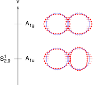
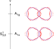
Figure 1: Odd and even vibrations of the dimer constructed from S${}_{\ell,0}^{1}$ modes of the free spheres with $\ell=2$ (left) and $\ell=3$ (right). The $z$-axis goes through the centers of both spheres and the 3D displacements are obtained by rotation around this axis.

Because the parity of the spheroidal vibrations is the same as the parity of $\ell$, the construction of the odd and even vibrations of the dimer is different for odd $\ell$ as illustrated in Fig. 1 for $\ell=3$ but the resulting even vibration of the dimer is always the one having different displacements for the two spheres at the center of the dimer and therefore the one having a larger frequency shift compared to the frequency of the free spheres.

The translation along $z$ for a single sphere corresponds to a vibration at zero frequency. From this mode, we can construct an in-phase oscillation of the dimer which corresponds to the translation along $z$ of the dimer (0 GHz). The out-of-phase oscillation corresponds to the lowest A_1g mode (67.4 GHz). To confirm this assignment we checked that the frequency of this A_1g mode tends to zero as the coupling between the spheres decreases. In order to have a finer control the magnitude of this coupling, we considered a dumbbell made of spheres connected by a cylinder whose radius is $r=R/10$. This small dimension ensures that the eigenfrequencies of the free cylinder are large which restricts the number of vibrations of the cylinder which can manifest in the low frequency range. Figure 2 shows the variation of the frequency of the lowest frequency A_1g mode as a function of the length of the cylinder $L$. Since the spheres are hardly deformed but rather translated during the oscillation, it is possible to model this oscillation as that of two point masses connected by a spring. While a first order perturbation theory for a massless spring is possible, we present here only a basic derivation valid for this particular vibration. The force constant of the massless equivalent spring equivalent to the cylinder is $k_{sp}=Y\frac{A}{L}$ where $Y$ is the Young’s modulus and the cross sectional area of the cylinder is $A=\pi r^{2}$. This expression is valid only for $L\gg r$. The resulting frequency for the dimer is then $\omega=\sqrt{2k_{sp}/M}$. The very good agreement observed in Fig. 2 for $L>4$ nm is an indication of both the validity of the assignment of this mode and the accuracy of the computation of the vibration eigenmodes even for such a challenging geometry. This particular oscillation is of interest since it was recently experimentally observed.TchebotarevaCPC09 The present work demonstrates that measuring its frequency is equivalent to determining the force constant of the “spring” which connects the two NPs constituting the dimer.

Figure 2: Frequency of the lowest A_1g mode calculated for two silver spheres of radii $R=5$ nm connected with a cylinder of radius $r=R/10=0.5$ nm and length $L$ ($N=20$ full circles, $N=18$ crosses, $N=16$ stars and $N=21$ full squares) compared to the frequency of two point masses connected with a spring having a force constant equal to that of the cylinder (line) using Eq. 24.

Table 2 presents a set of low-frequency modes $i=1-12$ originating from the translations (S${}_{1,m}^{0}$) and rotations (T${}_{1,m}^{0}$) of the spheres. Modes $i=1-6$ (not shown) correspond to the rotations and translations of the dimer with zero frequency. These 12 eigenmodes correspond to the number of rotations and translations of the two spheres. Then modes $i=13-32$ correspond to combinations of the S${}_{2,m}^{1}$ or T${}_{2,m}^{1}$ and so on. Again, these 20 eigenmodes correspond to the number of S${}_{2,m}^{1}$ and T${}_{2,m}^{1}$ eigenmodes of the two spheres. Modes corresponding to the superpositions of the breathing modes (S${}_{0,0}^{1}$) are also shown. However, since the vibrational density of states increases with frequency, even in this relatively low coupling case this mode mixes significantly with (S${}_{5,0}^{1}$). This mixing is not apparent in Table 2 since only the main contributions are shown. The same rule regarding the shift of the frequencies as discussed for the modes originating from S${}_{2,0}^{1}$ before applies for every modes.

The way the vibrations of a dimer are built is the analog of the way molecular orbitals are built using the linear combination of atomic orbitals (LCAO) method. Such an analogy has already been pointed out before in the case of acoustic waves in periodic ensemble of spheres in a host material.Kafesaki95 For example, the A_1u and A_1g modes built from the breathing mode of the spheres (S${}_{0,0}^{1}$) are analogous to the bonding and anti-bonding molecular orbital of H₂ built from the $1s$ orbitals. However the reduction in the energy of the bonding orbital compared to that of the $1s$ atomic orbital does not exist for the A_1u vibration since there is no acoustic equivalence for the screening of the charges of the nuclei due to the electrons.

In order to study the influence of the coupling of the vibrations of the two spheres, the variation of the frequencies of the different vibrations are plotted in Fig. 3 as a function of the distance between the center of the spheres. For $d=0$ the system consists of a single sphere and the frequencies match those reported in Table 1. For $d$ very close to $2R$, the behavior is singular because for $d=2R$ the two spheres touch at a single point. Moreover, for $d=2R-\epsilon$ each sphere feels the other sphere as a mass attached to it but it is no longer the case for $d=2R+\epsilon$. So despite the the convergence being good, the interpretation of the results is not obvious at this point since we can expect a non-smooth variation of the frequencies at $d=2R$. Figure 3 presents the branches corresponding to the situation when $d<2R$. The lines between the calculated frequencies connect eigenmodes having the same irreducible representation. This was also done in a previous work.SaviotPRB09 The mixings between the branches having the same irreducible representations are numerous and show that the nature of the vibrations in the case of a strong coupling can be quite complex.

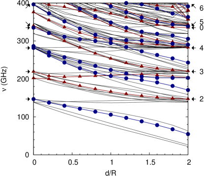
Figure 3: Variation of the frequencies of a dumbbell made of two silver spheres with radii $R=5$ nm with varying distance $d$ between their centers. The A_1g and A_1u branches are plotted with circles (blue online) and triangles (red online) respectively. The frequencies of some S${}^{1}_{\ell}$ modes are marked with arrows and labeled with $\ell$.

III.2 Convergence of the numerical method

The numerical method used in this work has been shown to be very accurate for several different geometries. The question of its reliability for the challenging systems in this work is addressed here. To that end, we performed the same calculations with $N=18$ (Table 2) and $N=16$ and $N=21$ (Figs. 2 and 4) to compare with the reference $N=20$. This comparison does not rely on the mode index $i$ but rather on the irreducible representation. For example, $\Delta\nu$ for mode $i=10$ in Table 2 is the frequency variation for the lowest frequency A_1g mode with $N=20$ and $N=18$. We varied $N$ by steps of 2 because adding or removing one to $N$ does not change the frequencies of all the eigenmodes. This is due to the inversion symmetry. Changing $N$ by one adds or removes even or odd functions only depending on the parity of $N$. Therefore only the convergence of even or odd modes is changed.

Figure 4: Frequency of the second lowest A_1g mode calculated for two silver spheres of radii $R=5$ nm connected with a narrow cylinder of radius $r=R/10=0.5$ nm and length $L$ ($N=20$ full circles, $N=18$ crosses, $N=16$ stars and $N=21$ full squares) compared to the first order perturbation calculation of the coupling of the S${}_{2,0}^{1}$ eigenmodes of the spheres through the extensional eigenmode of the thin cylinder (line) using Eq. 24.

The convergence for the results presented in Table 2 is good. This is due to the use of a rather high value for $N$. The largest variations $\Delta\nu$ are obtained for the lowest frequency modes. This tendency is confirmed by Figs. 2, 4 and 5 except for large values of $L$ for which the convergence for the lowest A_1g modes is much better. The worst convergence is for $L=2$ nm for which the variation between $N=20$ and $N=21$ in Fig. 5 is still quite large (9%). This can be understood when comparing the calculated displacements along the $z$-axis with that expected from the ideal spring model for which both spheres are translated in opposite directions and the displacement varies linearly inside the spring (see Fig. 5). The steep variation of this displacement inside the cylinder together with the flat variation inside the spheres are much more difficult to reproduce with power functions of $z$ when the length of the spring ($L$) is small. Moreover, for $L=2$ nm, $L/r=4$ so the behavior of the cylinder may differ from the spring approximation. The variation of the displacement for overlapping spheres is not so steep which explains why the convergence is much better in that case. Indeed, the spring approximation does not hold as can be checked from the displacement plotted in Fig. 5 (top). The deformation of each sphere is quite significant or in other words the coupling is not so weak. Similar comments apply for the other modes which are combinations of rotations and translations of the spheres with a non-zero frequency except that the relevant characteristic value of the cylinder is not related to its stretching but rather to torsion and bending. For the other modes at higher frequency, the displacements inside the spheres are not constant which can be easier to reproduce with power functions of $x$, $y$ and $z$. Therefore, the convergence can be better than for the eigenmodes made of the rotations and translations of the two spheres.

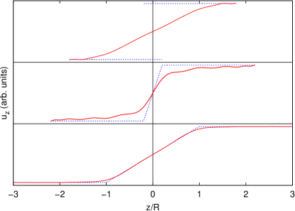
Figure 5: Normalized displacements along the $z$-axis for the lowest frequency A_1g mode of a dimer of overlapping spheres with d/R=1.6 (top) and of a cylindrical-necked dumbbell with cylinder length $L$ equal to 2 nm (middle) and 10 nm (bottom). Each sphere has radius 5 nm. The continuous lines correspond to the numerical results for $N=20$ while the dotted ones correspond to a constant displacement inside each sphere (translation along $z$) and a linear variation of the displacement inside the cylinder when it is present.

The convergence for the second lowest A_1g vibration was also checked using the same method. In that case, the calculations are compared with the first order perturbation results presented before for a thin cylinder. This is necessary because the extensional vibration of this cylinder has a frequency similar to the S${}_{2}^{1}$ vibration of the spheres for $L=2R=10$ nm. The comparison of both calculations in Fig. 4 shows the very high accuracy of the RUS calculations for long enough cylinders, i.e. when the approximations made for the perturbation theory are valid.

III.3 Non-symmetrical dimer

In this general case, there are some restrictions on which isolated sphere eigenvibrations can be combined to create a vibration eigenmode for the dimer. First, the two spheres’ vibrations should share the same irreducible representation in C_∞v (same $m$ and same character (S or T) for $m=0$) otherwise their superposition would not have a well-defined symmetry. Second, their frequencies should match because all the points inside the system oscillate at the same frequency for an eigenmode.

When going from a symmetric dimer to a non-symmetric one, the inversion symmetry is lost and the two spheres have different sets of vibrational frequencies. For example it is possible that the frequency of the S${}^{1}_{1,0}$ mode of one sphere might happen to match the frequency of the S${}^{1}_{2,0}$ mode of the other. In this case, some modes of the dimer as a whole would be hybridizations of these two. However, such an exact match of mode frequencies is very unlikely. Leaving aside such coincidences, in the very weak coupling regime the modes of the dimer are simply the superposition of one eigenmode for one sphere with the other sphere at rest because that is the only way to have all the points of the dimer oscillating at the same frequency. When the coupling becomes stronger the modes can be mixed even more than in the case of the symmetric dimer since parity is lost. In that case, any modes having the same value of $m$ can mix provided their frequencies are close except for $m=0$ for which torsional and spheroidal modes can not mix.

IV Conclusion

We have demonstrated that an exhaustive description of the vibrations of a weakly coupled dimer based on continuum calculations, perturbation theory and symmetry considerations is possible. While the strong coupling regime can be investigated using these numerical tools, it is of course quite hard to interpret the results since the free oscillations of the spheres constituting the dimer are strongly modified. The convergence of the calculations is discussed in the weak coupling regime thanks to the comparison with perturbation calculations and accurate results are obtained in most cases. General equations were given to extend the perturbation approach to other weakly coupled systems. This work paves the way for the understanding of the vibrations of more complex systems of interest such as chains of overlapping spheres as in nanocolumnsBurginNL08 and chains of non-spherical particles.

References

- (1) T. Takagahara, Phys. Rev. Lett. 71, 3577 (1993)
- (2) D. Oron, A. Aharoni, C. de Mello Donega, J. van Rijssel, A. Meijerink, and U. Banin, Phys. Rev. Lett. 102, 177402 (2009)
- (3) Y. Li, Q. Zhang, A. V. Nurmikko, and S. Sun, Nano Lett. 5, 1689 (2005)
- (4) A. L. Tchebotareva, M. A. van Dijk, P. V. Ruijgrok, V. Fokkema, M. H. S. Hesselberth, M. Lippitz, and M. Orrit, Chem. Phys. Chem. 10, 111 (2009)
- (5) T. Dehoux, T. A. Kelf, M. Tomoda, O. Matsuda, O. B. Wright, K. Ueno, Y. Nishijima, S. Juodkazis, H. Misawa, V. Tournat, and V. E. Gusev, Opt. Lett. 34, 3740 (2009)
- (6) J. Burgin, P. Langot, A. Arbouet, J. Margueritat, J. Gonzalo, C. N. Afonso, F. Vallée, A. Mlayah, M. D. Rossell, and G. Van Tendeloo, Nano Lett. 8, 1296 (2008)
- (7) A. Courty, A. Mermet, P. A. Albouy, E. Duval, and M. P. Pileni, Nature Materials 4, 395 (2005)
- (8) M. Ivanda, M. Buljan, U. V. Desnica, K. Furić, D. Ristić, G. C. Righini, and M. Ferrari, Advances in Science and Technology 55, 127 (2008)
- (9) C. Pighini, D. Aymes, N. Millot, and L. Saviot, J. Nanoparticle Research 9, 309 (2007)
- (10) D. B. Murray, C. H. Netting, L. Saviot, C. Pighini, N. Millot, D. Aymes, and H.-L. Liu, J. Nanoelectron. Optoelectron. 1, 92 (2006)
- (11) L. Saviot, C. H. Netting, D. B. Murray, S. Rols, A. Mermet, A.-L. Papa, C. Pighini, D. Aymes, and N. Millot, Phys. Rev. B 78, 245426 (2008)
- (12) L. Saviot and D. B. Murray, Phys. Rev. B 79, 214101 (2009)
- (13) B. C. Hathorn, B. G. Sumpter, D. W. Noid, R. E. Tuzun, and C. Yang, J. Phys. Chem. A 106, 9174 (2002)
- (14) N. Combe, P.-M. Chassaing, and F. Demangeot, Phys. Rev. B 79, 045408 (2009)
- (15) W. M. Visscher, A. Migliori, T. M. Bell, and R. A. Reinert, J. Acoust. Soc. Am. 90, 2154 (1991)
- (16) H. Portalès, N. Goubet, L. Saviot, S. Adichtchev, D. B. Murray, A. Mermet, E. Duval, and M.-P. Piléni, Proc. Natl. Acad. Sci. U.S.A 105, 14784 (2008)
- (17) M. Kafesaki and E. N. Economou, Phys. Rev. B 52, 13317 (1995)