Thermodynamics and short-range correlations of the XXZ chain close to its triple point

Abstract

The XXZ quantum spin chain has a triple point in its ground state $h$-$1/\Delta$ phase diagram. This first order critical point is located at the joint end point of the two second order phase transition lines marking the transition from the gapless phase to the fully polarized phase and to the Néel ordered phase, respectively. We explore the magnetization and the short-range correlation functions in its vicinity using the exact solution of the model. In the critical regime above the triple point we observe a strong variation of all physical quantities on a low energy scale of order $1/\Delta$ induced by the transversal quantum fluctuations. We interpret this phenomenon starting from a strong-coupling perturbation theory about the highly degenerate ground state of the Ising chain at the triple point. From the perturbation theory we identify the relevant scaling of the magnetic field and of the temperature. Applying the scaling to the exact solutions we obtain explicit formulae for the magnetization and short-range correlation functions at low temperatures.

1 Introduction

Critical points in the ground state phase diagram are nowadays often called quantum critical. In this terminology the triple point of the XXZ chain is a quantum critical point of first order. Quantum critical points have been proposed as a paradigm in condensed matter physics for explaining severe deviations in the behaviour of strongly correlated electrons from the Fermi liquid picture. Much of the intuitive understanding of quantum critical points comes from simple exactly solved models [11]. In this work we would like to extend the list of those quantum critical points that can be studied exactly by another example.

The ground state phase diagram of the XXZ chain in the $h$-$1/\Delta$ plane has three distinguished critical points. Two of them are the isotropic ferromagnetic and antiferromagnetic points at $h=0$ and $\Delta=-1$ or $\Delta=1$, respectively. Although the model is exactly solvable by Bethe ansatz, it is hard to calculate its thermodynamic properties in the vicinity of the ferromagnetic point. The antiferromagnetic point is easier to access, but still requires a certain effort in the numerical solution of the integral equations [13].

A third critical point, to which less attention has been paid, is the aforementioned triple point. It will be studied in this work. The triple point is located at $\Delta=\infty$ and $h=h_{c}$ with $\Delta$ denoting the anisotropy parameter of the XXZ model and $h_{c}$ the critical magnetic field separating between the fully polarized phase and the Néel phase of the Ising chain. This critical point is simpler than the other two, because degenerate strong-coupling perturbation theory can be applied in its vicinity. Applying the same perturbative expansion to the integral equations that determine the thermodynamics of the model [13] we obtain free fermion type equations for low temperatures and algebraic equations in the zero temperature limit. Those equations provide explicit results e.g. for the ground state magnetization and some static correlation functions up to first order in $1/\Delta$. On the other hand, treating the integral equations numerically, we obtain the exact temperature dependent picture, and we can assess the range of validity of the perturbation theory.

2 XXZ chain in the vicinity of the strong coupling critical point

We consider the XXZ Hamiltonian, which on the ‘gapped antiferromagnetic side’ of the phase diagram is most naturally written as

$$\mathcal{H}=\sum_{j=1}^{L}\left[J(\sigma_{j-1}^{z}\sigma_{j}^{z}-1)+\frac{J}{\Delta}(\sigma_{j-1}^{x}\sigma_{j}^{x}+\sigma_{j-1}^{y}\sigma_{j}^{y})-\frac{h}{2}\sigma_{j}^{z}\right]$$ (1)

with $J,h>0$ and $\Delta>1$. Here the $\sigma_{j}^{\alpha},\,j=1,\ldots,L$, $\alpha=x,y,z$, act locally as Pauli matrices, $J$ is the exchange coupling, $h$ denotes the strength of the magnetic field, and $\Delta=\operatorname{ch}(\eta)$ is the anisotropy parameter.

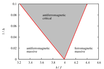
Figure 1: (Color online) Ground state phase diagram of the XXZ chain in the $h$-$1/\Delta$ plane for fixed $J$ and large $\Delta$ in the vicinity of the triple point.

The ground state phase diagram in the $h$-$1/\Delta$ plane can be obtained from the Bethe ansatz solution of the model (see e.g. [12]). We show a detail of it in figure 1. The lower critical field $h_{e}$ (left red line) is given by the excitation gap [6, 14] whereas the saturation field (right red line) is given by the simple explicit formula $h_{s}=4J(1+1/\Delta)$. These fields determine the second order phase transition lines between the critical and massive phases drawn in figure 1. The lines are asymptotically straight. For the lower critical field one can see deviations from the asymptotic behaviour $h_{e}\approx 4J(1-2/\Delta)$, but they are small on the scale used in the figure. The point $h=4J$, $\Delta=\infty$ in which the two second order phase transition lines join is the triple point we are interested in. In the following we shall characterize it starting with the Hamiltonian.

For $\Delta\rightarrow\infty$ the XXZ chain (1) simplifies to the Ising chain

$$\mathcal{H}_{I}(h)=\sum_{j=1}^{L}\left[J(\sigma_{j-1}^{z}\sigma_{j}^{z}-1)-\frac{h}{2}\sigma_{j}^{z}\right]=\frac{1}{2}\sum_{j=1}^{L}{\rm diag}(-h,-4J,-4J,h)_{j-1,j}\,,$$ (2)

which is diagonal in a basis of tensor products of local $S^{z}$-eigenstates. From the second equation we can easily understand how its ground states change with the magnetic field. If $h<4J$ the two Néel states consisting of alternating up- and down-spins are the ground states. If $h>4J$ the ground state is the unique fully polarized state with all spins pointing upwards. In the former case the ground state magnetization per lattice site vanishes, and in the latter case it is one half. Thus, there is a first order phase transition point at $h=h_{c}=4J$.

What happens exactly at the phase transition point? As can be seen from (2) all states with no neighbouring down-spins are degenerate and have lowest energy $-2JL$. Clearly their number is macroscopic in the thermodynamic limit where it is measured as the average number $s$ of states per site. We can obtain it from the known [3] entropy per site in the zero temperature limit. It is equal to the golden mean, $s=(1+\sqrt{5})/2$. All states with exactly two neighbouring down spins are the lowest excited states above the ground state with excitation energy $4J$. The magnetization per lattice site right at the critical point takes a value different from zero and one half, namely $m=1/2\sqrt{5}$.

Let us rewrite the Hamiltonian (1) as

$$\mathcal{H}=\mathcal{H}_{I}(h_{c})+\frac{J}{\Delta}\sum_{j=1}^{L}\left(\sigma_{j-1}^{x}\sigma_{j}^{x}+\sigma_{j-1}^{y}\sigma_{j}^{y}-2\alpha\sigma_{j}^{z}\right)$$ (3)

with $\alpha=\Delta(h/h_{c}-1)$. Then, for every fixed $\alpha$, the second term becomes small for sufficiently large $\Delta$ and can be viewed as a perturbation to the Hamiltonian $\mathcal{H}_{I}(h_{c})$. The splitting of the ground state under the influence of the perturbation can be understood by means of an effective Hamiltonian obtained in second order degenerate perturbation theory, in a similar way as e.g. the Heisenberg Hamiltonian is obtained from the Hubbard Hamiltonian at half band-filling in the strong coupling limit (see e.g. appendix 2.A of [7]). Note that curves of fixed $\alpha$ are straight lines originating from the critical point at $h=h_{c}$ and $\Delta=\infty$ in figure 1.

Using second order degenerate perturbation theory we obtain the effective Hamiltonian

$$\mathcal{H}=-2JL+\frac{J}{\Delta}P_{0}\sum_{j=1}^{L}\left(\sigma_{j-1}^{x}\sigma_{j}^{x}+\sigma_{j-1}^{y}\sigma_{j}^{y}-2\alpha\sigma_{j}^{z}\right)P_{0}\\ -\frac{J}{\Delta^{2}}P_{0}\sum_{j=1}^{L}\left[\frac{1}{2}\left(1-\sigma_{j-1}^{z}\right)\left(1-\sigma_{j+1}^{z}\right)+\left(\sigma_{j-2}^{+}\sigma_{j-1}^{-}\sigma_{j}^{+}\sigma_{j+1}^{-}+h.c.\right)\right]P_{0}\,,$$ (4)

describing the splitting of the ground state. Here $P_{0}$ is the projector onto the subspace with no neighbouring down-spins. Note that the magnetic field does not enter into the second order correction.

The first order term, let us call it $\mathcal{H}_{1}$, is an integrable Hamiltonian [2] in full analogy with the situation with the one-dimensional Hubbard model in the strong coupling limit. The operator $\rho_{1}={\rm e}^{-J\mathcal{H}_{1}/\Delta T}/\operatorname{tr}{\rm e}^{-J\mathcal{H}_{1}/\Delta T}$ replaces the statistical operator to lowest order in $J/\Delta$. For $T\rightarrow 0+$ it becomes the projector onto the ground state of $\mathcal{H}_{1}$. It follows that, to leading order, the ground state correlation functions depend only on $\alpha$, i.e. they are constant on straight lines originating from the triple point. Their values on lines parallel to the $h$-axis in figure 1 must vary continuously between the values taken at the boundaries between the massive and the massless phases marked by the second order phase transition lines. The value of the magnetization per lattice site, in particular, calculated in the limit $\Delta\rightarrow\infty$ on straight lines of fixed $\alpha$, must vary continuously between zero and one half, which already gives us a precise picture of the nature of the singularity of the first order quantum critical point.

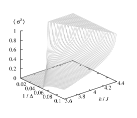
Figure 2: Magnetization of the XXZ chain close to the triple point for $T\rightarrow 0$.

Considering the finite temperature physics of the effective Hamiltonian (4) for fixed $\alpha$ we see that, to leading order, the anisotropy $\Delta$ appears only as a prefactor, i.e. as a new temperature scale. This can be utilized by introducing a rescaled temperature $\tau=\Delta T$. Keeping $\alpha$ and $\tau$ fixed and sending $\Delta$ to infinity removes all corrections to ${\cal H}_{1}$. In this limit the original XXZ Hamiltonian is replaced by ${\cal H}_{1}$. The form of the effective Hamiltonian implies that this should be justified as long as $\Delta$ is large enough, say $\Delta>10$, since then the second term in (4) becomes small compared to ${\cal H}_{1}$. At the same time the temperature $T$ must be small compared to the excitation gap $4J$ of ${\cal H}_{I}(h_{c})$ for the perturbation theory to be applicable.

As we have seen, our strong-coupling analysis provides a complete qualitative picture of the ground state correlation functions in the region of the phase diagram above the triple point. Clearly, their values in leading order can be calculated using the exact solution of $\mathcal{H}_{1}$. Here we will proceed differently. We will take our previous results for the XXZ chain [13], already conveniently formulated in terms of integral equations, and consider them in the zero temperature limit and in the scaling limit. This way we obtain new and explicit results for the magnetization and some short-range correlation functions. They are shown in the following sections.

The magnetization and the short-range correlation function in the full phase diagram of the antiferromagnetic XXZ chain ($\Delta>-1$, $h$ and $T$ arbitrary) in the thermodynamic limit can be obtained by means of the formulae derived in [4, 13]. This only requires to solve certain well-behaved linear and non-linear integral equations numerically and can be done to arbitrary numerical precision. Examples were worked out in [4, 13]. In [13], in particular, we noticed the extreme variation of the short-distance correlation functions close to the triple point. Meanwhile we have worked this out in more detail.

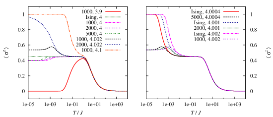
Figure 3: (Color online) The one-point function $\left<\sigma^{z}\right>$ for large values of the anisotropy, fixed $J$ and different values of $h/J$. The labels in the panels are the tuples $\Delta,h/J$ where ‘Ising’ denotes the analytic Ising curves.

In [13] we discussed the temperature behaviour of two-point correlation functions, e.g. of the connected correlation function $\langle\sigma_{1}^{z}\sigma_{3}^{z}\rangle-\langle\sigma_{1}^{z}\rangle\langle\sigma_{3}^{z}\rangle$. It turns out, however, that the signature of the quantum critical point is most clearly observed in the magnetization per site (which is the only non-vanishing one-point function), as it is monotonic in the magnetic field. We show it in figures 3 and 2. In addition, the two-point functions for two and three sites are shown in figure 4. Note that the non-vanishing of the transversal correlation functions in the zero temperature limit is due to the residual quantum mechanical interactions for finite $\Delta$.

The left panel in figure 3 shows how small changes in the magnetic field or in the coupling $1/\Delta$ induce large changes in the low temperature behaviour of the one-point function $\langle\sigma_{j}^{z}\rangle$ due to the proximity of the triple point. The critical cone above the triple point corresponds to $\alpha\in[-2,1]$ (see below). The point $\Delta=1000$, $h=4.1$ is outside the critical cone on the massive fully polarized side, while $\Delta=1000$, $h=3.9$ corresponds to a point on the massive antiferromagnetic side of the phase diagram in figure 1. All other curves in the left panel of figure 3 belong to various values of $\alpha\in[-2,1]$. The curves for $h/J=4$, i.e. for $h=h_{c}$, in particular, correspond to $\alpha=0$. It can be seen in the figure how, for increasing $\Delta$, these curves become more and more similar to the curve for the Ising model at the critical point, but for small enough temperature always deviate from the value $\langle\sigma_{j}^{z}\rangle=1/\sqrt{5}$ of the one-point function of the Ising chain.

In the right panel of figure 3 we compare curves with different values of the magnetic field and $\alpha=0.5$ and curves for the Ising model with the same values of the magnetic field. We can identify four different temperature regimes. For very high temperatures $T\gg h$ the curves are independent of $\Delta$ and $h$. Then, for intermediate temperatures $T\approx h$, they are independent of the (large) anisotropy and only depend on the magnetic field. This is where the curves for finite $\Delta$ and the curves of the Ising model match. We expect that this regime extends down to $T\approx 10J/\Delta$, where the thermal fluctuations still dominate the transversal quantum fluctuations. Next comes a regime $T\approx J/\Delta$, where thermal fluctuations and transversal quantum fluctuations are of the same order of magnitude. Here the correlation functions depend on the anisotropy and the magnetic field. The different curves in this regime match, if one introduces the rescaled temperature $\tau=T\Delta$, see section 4. Finally, for very low temperatures $T\ll J/\Delta$, the product $\alpha=\Delta(h/h_{c}-1)$ determines the value of the correlation functions. This case will be worked out explicitly in the next section.

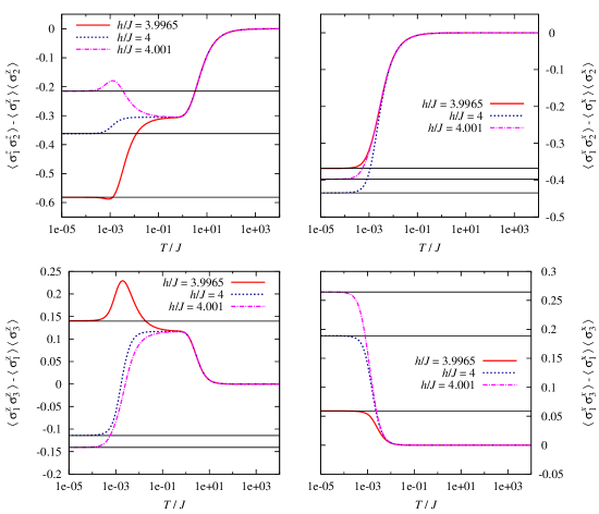
Figure 4: (Color online) The temperature dependence of the two-point functions for two and three neighbouring sites are shown for different values of the magnetic field for $\Delta=1000$. Additionally, the zero temperature asymptotic values obtained in (15) are shown as black lines.

3 Zero temperature limit

In the following we shall work out explicit formulae for the zero temperature asymptotics of the magnetization and of a few neighbour two-point functions on lines of constant $\alpha=\Delta(h/h_{c}-1)$ in the vicinity of the triple point. We shall resort to our previous work [13] in which we studied the XXZ chain for $\Delta>1$. The simple idea is to perform the zero temperature limit for large $\Delta$ and fixed $\alpha$ in the special functions of [13] that characterize the correlation functions. For this purpose the form of the non-linear integral equations as used in [5] is slightly more convenient than that of [13], for, in the zero temperature limit, where the integral equations become linear, the range of integration is over the Fermi sea and not over its complement. For large $\Delta$, finally, the linear integral equations turn into algebraic equations.

Referring to [8, 13], where certain auxiliary functions $\bar{\mathfrak{b}}$ and $\mathfrak{a}$ were explained, we introduce the familiar dressed energy $\varepsilon$ obtained in our setting from $\bar{\mathfrak{b}}$ or $\mathfrak{a}$ in the zero temperature limit,

$$\varepsilon(x)=\lim_{T\rightarrow 0}T\ln\bar{\mathfrak{b}}(x)=\lim_{T\rightarrow 0}-T\ln\mathfrak{a}({\rm i}x-\eta/2)\,.$$ (5)

It satisfies the integral equation (see e.g. [8])

$$\varepsilon(x)=h-4J\operatorname{sh}(\eta)K_{\eta/2}(x)-\int_{-\Lambda}^{\Lambda}\frac{\mathrm{d}y}{\pi}K_{\eta}(x-y)\varepsilon(y)$$ (6)

with

$$K_{\eta}(x)=\frac{\operatorname{sh}(2\eta)}{2\sin(x+{\rm i}\eta)\sin(x-{\rm i}\eta)}$$ (7)

and $\varepsilon(\pm\Lambda)=0$.

Now we use $h=h_{c}\left(1+\frac{\alpha}{\Delta}\right)$ and expand the equation up to the order $1/\Delta$. Then

$$\varepsilon(x)=\frac{h_{c}\alpha}{\Delta}-\frac{h_{c}\cos(2x)}{\Delta}-\int_{-\Lambda}^{\Lambda}\frac{\mathrm{d}y}{\pi}\>\varepsilon(y)$$ (8)

which can be solved explicitly,

$$\varepsilon(x)=\frac{h_{c}}{\Delta}\left(\frac{\alpha+\sin(\pi c)/\pi}{1+c}-\cos(2x)\right)$$ (9)

with $c=\frac{2}{\pi}\Lambda$. The Fermi points $\pm\Lambda$ or $\pm c$, respectively, are determined by the rescaled magnetic field $\alpha$,

$$\alpha=(1+c)\cos(\pi c)-\frac{1}{\pi}\sin(\pi c)\,.$$ (10)

Here $c$ is a monotonic function of $\alpha$ for $\alpha\in[-2,1]$. The boundaries $-2$ and $1$ of the interval correspond to the phase transition lines (red lines in figure 1) determined to the order $1/\Delta$. For magnetic fields smaller than the lower critical field $h_{e}$ or larger than the saturation field $h_{s}$ the ground state and, hence, the Fermi points are independent of $h$.

The ground state energy $e$ is given by

$$e= -\frac{h}{2}+\int_{-\Lambda}^{\Lambda}\frac{\mathrm{d}y}{\pi}K_{\eta/2}(y)\varepsilon(y)$$ (11)

$$\approx -\frac{h_{c}}{2}\left(1+\frac{\alpha}{\Delta}\right)-\frac{h_{c}}{\Delta}\frac{\frac{1}{\pi}\sin(\pi c)-\alpha c}{1+c}\,.$$ (12)

Using it one obtains for the magnetization in leading order

$$m=\frac{\langle\sigma^{z}\rangle}{2}=\frac{1-c}{2(1+c)}\,.$$ (13)

Then the leading order magnetic susceptibility is

$$\chi=\frac{\Delta}{h_{c}}\frac{1}{(1+c)^{3}\sin(\pi c)}\,.$$ (14)

We see that it diverges at the critical point.

In a similar way one can take the zero temperature limit for the functions that determine the correlation functions, e.g. for $\omega$ and $\omega^{\prime}$ defined in [13] and for the auxiliary functions stemming from linear integral equations (see the appendix, where the zero temperature limit is obtained from the low temperature approximation discussed in the next section). This leads to the following expressions for the zero temperature correlation functions

$$\left\langle\sigma_{1}^{z}\sigma_{2}^{z}\right\rangle_{h}= \frac{1-3c}{1+c}\,,$$ (15a)

$$\left\langle\sigma_{1}^{x}\sigma_{2}^{x}\right\rangle_{h}= -\frac{2\sin(\pi c)}{\pi(1+c)}\,,$$ (15b)

$$\left\langle\sigma_{1}^{z}\sigma_{3}^{z}\right\rangle_{h}= \frac{1-3c+4c^{2}}{1+c}-\frac{4\sin^{2}(\pi c)}{\pi^{2}(1+c)}\,,$$ (15c)

$$\left\langle\sigma_{1}^{x}\sigma_{3}^{x}\right\rangle_{h}= \frac{2\sin^{2}(\pi c)}{\pi^{2}(1+c)}-\frac{2c\sin(2\pi c)}{\pi(1+c)}+\frac{\sin(2\pi c)}{\pi}\,.$$ (15d)

In figure 4 we show that the asymptotic values of the zero-temperature correlation functions match indeed the low temperature behaviour of the temperature dependent correlation functions calculated numerically from the integral equations as described in [13].

In figure 5 we show the dependence of the correlation functions as calculated in (15) on the rescaled magnetic field $\alpha$. In addition the normalized Fermi point $c$ is shown as a function of $\alpha$. Both, the Fermi point $c$ and the one-point function $\langle\sigma^{z}\rangle$, are monotonic functions of the magnetic field. The connected two-point function $\left\langle\sigma_{1}^{z}\sigma_{2}^{z}\right\rangle-\left\langle\sigma_{1}^{z}\right\rangle\left\langle\sigma_{2}^{z}\right\rangle$ is monotonic as well. The other correlation functions in the figure, however, show non-monotonic behaviour. Both two-point functions have their extremum above the critical field of the Ising chain, whereas the minimum of $\left\langle\sigma_{1}^{x}\sigma_{2}^{x}\right\rangle$ is exactly at the critical field of the Ising chain.

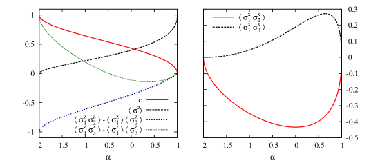
Figure 5: (Color online) The asymptotic values of the zero temperature correlation functions according to equation (15) are shown as a functions of the rescaled magnetic field $\alpha$. In addition we show the normalized Fermi point $c$ as a function of $\alpha$.

4 Low temperature behaviour

After the discussion of the zero temperature limit in the previous section which gave the correct scaling behaviour of the magnetic field, we would like to discuss small but finite temperatures. For this purpose we introduce a new rescaled temperature $\tau=\Delta T$ and expand the integral equations to lowest non-vanishing order in $1/\Delta$ with $\tau$ and $\alpha$ kept fix. This leads to

$$\varepsilon(x)=h_{c}\alpha-h_{c}\cos(2x)+\int_{-\pi/2}^{\pi/2}\frac{\mathrm{d}y}{\pi}\>\tau\ln\left(1+{\rm e}^{-\varepsilon(y)/\tau}\right)$$ (16)

where $\varepsilon(x)$ is the finite temperature generalization of (5) in the scaling limit. Therefore we use the same notation for this function. We see that only one interval $[-\pi/2,\pi/2]$ of the original contour in the non-linear integral equation for the full XXZ chain [5] survives the limit. The contribution of the remaining part of the contour is exponentially suppressed for $\Delta\rightarrow\infty$.

The solution of the equation (16) is nothing but the dispersion relation of free fermions on the lattice

$$\varepsilon(x)=\mu-h_{c}\cos(2x)\,,$$ (17)

however, with a chemical potential $\mu$ which depends non-trivially on magnetic field and temperature and which is implicitly determined by the equation

$$\mu=h_{c}\alpha+\int_{-\pi/2}^{\pi/2}\frac{\mathrm{d}y}{\pi}\>\tau\ln\left(1+{\rm e}^{-(\mu-h_{c}\cos(2y))/\tau}\right)\,.$$ (18)

The free energy in this approximation is then given by

$$f=-\frac{h_{c}}{2}\left(1+\frac{\alpha}{\Delta}\right)+\frac{1}{\Delta}\int_{-\pi/2}^{\pi/2}\frac{\mathrm{d}y}{\pi}\>\tau\ln\left(1+{\rm e}^{-(\mu-h_{c}\cos(2y))/\tau}\right)$$ (19)

as for free fermions. Defining

$$I_{n}=\int_{-\pi/2}^{\pi/2}\frac{{\rm d}y}{\pi}\frac{\cos(2ny)}{1+{\rm e}^{(\mu-h_{c}\cos(2y))/\tau}}\,.$$ (20)

the magnetization follows as

$$m=\frac{1-I_{0}}{2(1+I_{0})}\,.$$ (21)

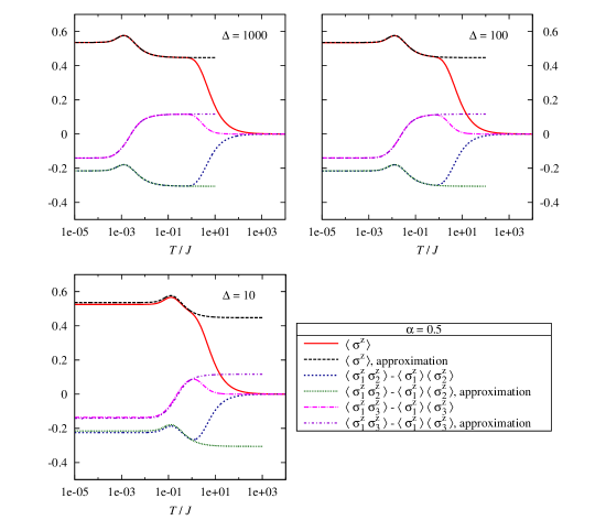
Figure 6: (Color online) The longitudinal correlation functions for short distances as a function of the temperature are shown for different values of the anisotropy and $\alpha=0.5$.

The calculation of the two-point functions within the same approximation is sketched in the appendix. We obtain

$$\left\langle\sigma_{1}^{z}\sigma_{2}^{z}\right\rangle_{\tau,h}= \frac{1-3I_{0}}{1+I_{0}}\,,$$ (22a)

$$\left\langle\sigma_{1}^{x}\sigma_{2}^{x}\right\rangle_{\tau,h}= -\frac{2I_{1}}{1+I_{0}}\,,$$ (22b)

$$\left\langle\sigma_{1}^{z}\sigma_{3}^{z}\right\rangle_{\tau,h}= \frac{1-3I_{0}+4I_{0}^{2}}{1+I_{0}}-\frac{4I_{1}^{2}}{1+I_{0}}\,,$$ (22c)

$$\left\langle\sigma_{1}^{x}\sigma_{3}^{x}\right\rangle_{\tau,h}= \frac{2I_{1}^{2}}{1+I_{0}}-\frac{4I_{0}I_{2}}{1+I_{0}}+2I_{2}\,.$$ (22d)

An important remark is that the structure of the two-point functions (22), unlike the structure of the free energy, is not the same as for free fermions. They rather depend on the density-density two-point functions $I_{n}$ for free fermions in an interesting way.

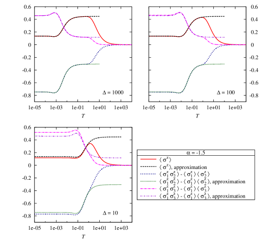
Figure 7: (Color online) The longitudinal correlation functions for short distances as a function of the temperature are shown for different values of the anisotropy and $\alpha=-1.5$.

In figure 6 and 7 the short-range longitudinal correlation functions are shown for fixed $\alpha$ and different values of the anisotropy. The exact solutions are compared with the solutions obtained within the scaling approximation. The agreement is surprisingly good. The approximate formulae hold up to $T\approx J$. This is compatible with the fact that the degenerate perturbation theory should be valid as long as the temperature is small compared to the excitation gap $4J$. Alternatively we can understand this fact from the perturbative treatment of the integral equations. As stated above and explained in some more detail in the appendix, the contribution of the second contour to the integral equation is exponentially suppressed with $\Delta$ for small enough $\tau$. On the scale of the true temperature $T$ this means that it behaves like $\exp(-J/T)$, i.e., in particular, in a way independent of $\Delta$.

In order to understand the strange high temperature behaviour of the correlation functions in the scaling limit, we have to recall that they are the exact correlation functions of the Hamiltonian ${\cal H}_{1}$, which is defined on the restricted Hilbert space with all configurations containing neighbouring down-spins excluded. In the high temperature limit, where statistical physics means to simply average over all possible configurations, the excess of up-spin electrons becomes visible in a non-vanishing magnetization. We can see in the figure that its high temperature value becomes independent of the anisotropy, as expected. Similarly, projecting out configurations with neighbouring down-spins means that it becomes more likely to have antiparallel neighbours, which causes the longitudinal neighbour-correlation function to be negative.

The scaling approximation applies to a wide range of the anisotropy. For $\Delta=100$ and $\Delta=1000$ the deviation from the exact solution is hardly recognizable, and the approximation is still in good qualitative agreement with the exact solution for $\Delta=10$. Comparing the cases $\alpha=0.5$ in figure 6 and $\alpha=-1.5$ in figure 7 one sees that for $\Delta=10$ the offset in the zero temperature limit is larger in the latter case. This is in agreement with the observation that the critical lines in the zero-temperature phase diagram in figure 1 relate differently to $\alpha$. The phase transition line to the fully polarized state belongs exactly to $\alpha=1$, while the line marking the transition to the Néel phase belongs to $\alpha=-2$ only asymptotically and deviations become visible for $\Delta\approx 10$. For this reason we generally expect larger deviations for smaller $\alpha\in[-2,1]$.

In general both figures show that in the regime $T\approx J/\Delta$, in which the correlation functions depend on the anisotropy and the magnetic field, the dependence on the anisotropy can be removed by introducing the rescaled temperature $\tau$. Since the scaling approximation is valid for temperatures up to $T\approx J$ and since the XXZ chain is well approximated by the Ising chain for temperatures higher then $T\approx 10J/\Delta$, the critical regime of the XXZ chain above the triple point is fully accessible by simple approximations (either Ising or ${\cal H}_{1}$) as long as $\Delta>10$. Outside the critical cone the Ising approximation works well for $\Delta>10$ and all temperatures anyway.

5 Conclusion

Based on the exact solution for the thermodynamics and short-distance correlation functions [13] we have examined the vicinity of the triple point of the XXZ chain in the critical regime. The low temperature physics in this region of the phase diagram and the nature of the singularity at the critical point can be understood qualitatively be means of degenerate perturbation theory around the ground state of the critical Hamiltonian ${\cal H}_{I}(h_{c})$. From the form of the second order effective Hamiltonian (4) it follows that a small scale $T\approx J/\Delta$ exists on which the correlation functions show strong variations and that below this scale the correlation functions must be constant on straight lines of fixed $\alpha=\Delta(h/h_{c}-1)$. Using the exact solution, formulated in terms of certain linear and non-linear integral equations [13], we have obtained a full quantitative understanding of the vicinity of the critical point at any temperature. We have seen that, as long as $\Delta>10$ the full XXZ Hamiltonian in the critical phase above the triple point is well approximated by the effective Hamiltonian ${\cal H}_{1}$ as long as $T<J$ and by $H_{I}(h_{c})$ for $T>10J/\Delta$. In particular, for the interesting intermediate and low temperature regime $T<J$ it is enough to consider ${\cal H}_{1}$. This is interesting, since ${\cal H}_{1}$ belongs to the relatively simple class of Hamiltonians similar to the impenetrable Bose gas [2]. The Bethe ansatz solution of models in this class is simple enough to admit for the derivation of finite temperature dynamical correlation functions in a closed form called determinant representation [10]. A determinant representation for ${\cal H}_{1}$ was derived in [1]. It could be the future starting point for an analysis of the asymptotic behaviour of the dynamical correlation functions in temperature regions in which conformal field theory is no longer a valid approximation. Such an analysis would be complementary to the perturbative study of the finite temperature dynamical correlation functions in the massive Néel ordered regime recently presented in [9].

Appendix: Low temperature approximation and zero temperature limit of the linear integral equations

We are referring to the notation and definitions of [13]. In order to calculate the low temperature limit of the two-point functions we have to begin with the functions $G$ and $G^{\prime}$. For these functions a shift as in (5) has to be made. We define

$$g^{-}_{\nu}(x):=-G({\rm i}x-\eta/2,{\rm i}\nu)\,,\quad{g^{\prime}}^{-}_{\nu}(x):=-\frac{G^{\prime}({\rm i}x-\eta/2,{\rm i}\nu)}{\eta}$$ (23)

which is consistent with the notation used in [13] except for the denominator $\eta$ in the second equation introduced for convenience here.

In the low temperature limit for large $\Delta$ the linear integral equations for $G$ and $G^{\prime}$ imply

$$g_{\nu}^{-}(x) =-2K_{\eta/2}(x-\nu)-\int_{-\pi/2}^{\pi/2}\frac{\mathrm{d}y}{\pi}K_{\eta}(x-y)\frac{g_{\nu}^{-}(y)}{1+{\rm e}^{(\mu-h_{c}\cos(2y))/\tau}}\,,$$ (24a)

$${g^{\prime}}_{\nu}^{-}(x) =-{\rm i}\,{\rm ctg}\,(x-\nu-\frac{{\rm i}\eta}{2})-\int_{-\pi/2}^{\pi/2}\frac{\mathrm{d}y}{\pi}L_{\eta}(x-y)\frac{g_{\nu}^{-}(y)}{1+{\rm e}^{(\mu-h_{c}\cos(2y))/\tau}}$$

$$\mspace{216.0mu}-\int_{-\pi/2}^{\pi/2}\frac{\mathrm{d}y}{\pi}K_{\eta}(x-y)\frac{{g^{\prime}}_{\nu}^{-}(y)}{1+{\rm e}^{(\mu-h_{c}\cos(2y))/\tau}}\,,$$ (24b)

where

$$L_{\eta}(x)=\frac{{\rm i}\sin(2x)}{2\sin(x+{\rm i}\eta)\sin(x-{\rm i}\eta)}\,.$$ (25)

The second part of the integration contour vanishes in this limit as it gives only exponentially small contributions for $\Delta\rightarrow\infty$, similar to (16).

We solve these equations up to the order $\exp(-2\eta)$ and obtain

$$g_{\nu}^{-}(x)=-\frac{2}{1+I_{0}}+{\rm e}^{-\eta}\left[\frac{4I_{1}}{1+I_{0}}\cos(2\nu)-4\cos(2(x-\nu))\right]$$

$$\mspace{48.0mu}+{\rm e}^{-2\eta}\left[\frac{4I_{2}}{1+I_{0}}\cos(4\nu)-\frac{4I_{1}^{2}}{(1+I_{0})^{2}}-4\cos(4(x-\nu))+\frac{4I_{1}}{1+I_{0}}\cos(2x)\right]\,,$$ (26a)

$${g^{\prime}}_{\nu}^{-}(x)=\frac{1}{1+I_{0}}+{\rm e}^{-\eta}\left[2{\rm e}^{-{\rm i}2(x-\nu)}-\frac{2I_{1}}{1+I_{0}}{\rm e}^{{\rm i}2\nu}\right]+{\rm e}^{-2\eta}\biggl{[}2{\rm e}^{-{\rm i}4(x-\nu)}$$

$$\mspace{135.0mu}\left.+\frac{{\rm i}4I_{1}}{1+I_{0}}\sin(2x)-\frac{2I_{1}}{1+I_{0}}\cos(2x)-\frac{2I_{2}}{1+I_{0}}{\rm e}^{{\rm i}4\nu}+\frac{2I_{1}^{2}}{(1+I_{0})^{2}}\right]\,.$$ (26b)

Finally we need the low temperature limit of $\omega$ and $\omega^{\prime}$ defined in [13]. One easily finds that

$$\omega(\nu_{1},\nu_{2})=K_{\eta}(\tilde{\nu}_{1}-\tilde{\nu}_{2})+2\int_{-\pi/2}^{\pi/2}\frac{\mathrm{d}x}{\pi}K_{\eta/2}(x-\tilde{\nu}_{2})\frac{g_{\tilde{\nu}_{1}}^{-}(x)}{1+{\rm e}^{(\mu-h_{c}\cos(2x))/\tau}}\,,$$ (27a)

$$\frac{\omega^{\prime}(\nu_{1},\nu_{2})}{\eta}=-L_{\eta}(\tilde{\nu}_{1}-\tilde{\nu}_{2})-\int_{-\pi/2}^{\pi/2}\frac{\mathrm{d}x}{\pi}{\rm i}\,{\rm ctg}\,(x-\tilde{\nu}_{2}-{\rm i}\eta/2)\frac{g_{\tilde{\nu}_{1}}^{-}(x)}{1+{\rm e}^{(\mu-h_{c}\cos(2x))/\tau}}$$

$$\mspace{270.0mu}+2\int_{-\pi/2}^{\pi/2}\frac{\mathrm{d}x}{\pi}K_{\eta/2}(x-\tilde{\nu}_{2})\frac{{g^{\prime}}_{\tilde{\nu}_{1}}^{-}(x)}{1+{\rm e}^{(\mu-h_{c}\cos(2x))/\tau}}\,,$$ (27b)

where we used the notation $\tilde{\nu}_{j}=-{\rm i}\nu_{j}$. Inserting (26) here and using equations (24) and (25) of [13] we obtain the equations (22).

For the zero temperature limit integrals over the Fermi weight of the form

$$\int_{-\pi/2}^{\pi/2}\frac{\mathrm{d}x}{\pi}\>\frac{f(x)}{1+{\rm e}^{(\mu-h_{c}\cos(2x))/\tau}}$$ (28)

have to be changed into integrals over the Fermi sea

$$\int_{-\Lambda}^{\Lambda}\frac{\mathrm{d}x}{\pi}\>f(x)\,.$$ (29)

The functions $I_{n}$, for instance, that determine the correlation functions in the low temperature scaling approximation have the following zero temperature limit

$$I_{0} \rightarrow c\,,$$ (30a)

$$I_{1} \rightarrow\frac{\sin(\pi c)}{\pi}\,,$$ (30b)

$$I_{2} \rightarrow\frac{\sin(2\pi c)}{2\pi}\,.$$ (30c)

With this limit introduced into (22) one obtains the zero temperature correlation functions (15).

References

- [1] N. I. Abarenkova and A. G. Pronko, Temperature correlation function in the absolutely anisotropic XXZ Heisenberg chain, Theor. Math. Phys. 131 (2002), 690.
- [2] F. C. Alcaraz and R. Z. Bariev, An Exactly Solvable Constrained XXZ Chain, Statistical Physics in the Eve of the 21st Century (Series on Advances in Statistical Mechanics) (M. T. Bachelor and L. T. Wille, eds.), vol. 14, World Scientific, Singapore, 1999, cond-mat/9904042.
- [3] R. J. Baxter, Exactly solved models in statistical mechanics, Academic Press, London, 1982.
- [4] H. Boos, J. Damerau, F. Göhmann, A. Klümper, J. Suzuki, and A. Weiße, Short-distance thermal correlations in the XXZ chain, J. Stat. Mech. (2008), P08010.
- [5] H. Boos, F. Göhmann, A. Klümper, and J. Suzuki, Factorization of the finite temperature correlation functions of the XXZ chain in a magnetic field, J. Phys. A 40 (2007), 10699.
- [6] J. Des Cloizeaux and M. Gaudin, Anisotropic Linear Magnetic Chain, J. Math. Phys. 7 (1966), 1384.
- [7] F. H. L. Essler, H. Frahm, F. Göhmann, A. Klümper, and V. E. Korepin, The One-Dimensional Hubbard Model, Cambridge University Press, 2005.
- [8] F. Göhmann, A. Klümper, and A. Seel, Integral representations for correlation functions of the XXZ chain at finite temperature, J. Phys. A 37 (2004), 7625.
- [9] A. J. A. James, W. D. Goetze, and F. H. L. Essler, Finite temperature dynamical structure factor of the Heisenberg-Ising chain, Phys. Rev. B 79 (2009), 214408.
- [10] V. E. Korepin, N. M. Bogoliubov, and A. G. Izergin, Quantum inverse scattering method and correlation functions, Cambridge University Press, 1993.
- [11] Subir Sachdev, Quantum phase transitions, Cambridge University Press, 2000.
- [12] M. Takahashi, Thermodynamics of one-dimensional solvable models, Cambridge University Press, 1999.
- [13] C. Trippe, F. Göhmann, and A. Klümper, Short-distance thermal correlations in the massive XXZ chain, preprint, arXiv:0908.2233, 2009, to appear in EPJ B.
- [14] C. N. Yang and C. P. Yang, One-dimensional chain of anisotropic spin-spin interactions. III. Applications, Phys. Rep. 151 (1966), 258.