Colloquium: Phase transitions in polymers and liquids in electric fields

Abstract

The structure and thermodynamic state of a system changes under the influence of external electric fields. Neutral systems are characterized by their dielectric constant $\varepsilon$, while charged ones also by their charge distribution. In this Colloquium several phenomena occurring in soft-matter systems in spatially uniform and nonuniform fields are surveyed and the role of the conductivity $\sigma$ and the linear or nonlinear dependency of $\varepsilon$ on composition are identified. Uniform electric fields are responsible for elongation of droplets, for destabilization of interfaces between two liquids, and for mixing effects in liquid mixtures. Electric fields, when acting on phases with mesoscopic order, also give rise to block copolymer orientation, to destabilization of polymer-polymer interfaces, and to order-order phase transitions. The role of linear and nonlinear dependences of $\varepsilon$ on composition will be elucidated in these systems. In addition to the dielectric anisotropy, existence of a finite conductivity leads to appearance of large stresses when these systems are subject to external fields and usually to a reduction in the voltages required for the instabilities or phase transitions to occur. Finally, phase transitions which occur in nonuniform fields are described and emphasis on the importance of $\varepsilon$ and $\sigma$ is given.

I Introduction

There are numerous ways the structure and phase of a system can be influenced by external fields. The gravitational field can lead to changes in structure and composition, and in many cases even to phase transitions. However, while omnipresent on Earth, its effect is usually quite small. A magnetic field has several advantages, but it is also weak unless the system is magnetic. Shear forces are effective in changing the phase and structure of soft materials, but their presence is undesired in many cases. Electric fields, on the other hand, have several interesting properties: they have a strong effect even on neutral materials, they can be switched on or off, and they are ideally suited for the nanoworld, because an electric field increases linearly with a decrease in the electrode size, for a given electrode potential.

The subject of this Colloquium is the influence that electric fields have on interfaces between two liquids or polymers. This is a broad subject and we do not aim at fully covering it but rather mention in this review the main effects. An electric field deforms the interface and may give rise to a dynamical instability. Similarly, fields tend to orient ordered phases of heterogeneous polymeric materials in such a way as to minimize the electrostatic energy. Uniform electric fields can also lead to the creation of interfaces between liquids. Lastly, spatially nonuniform fields have a strong influence on the thermodynamic properties of liquid and surfactant mixtures.

We adopt a continuum coarse-grained approach, where all quantities vary smoothly enough to be described by continuous fields. In addition, interfaces between two pure immiscible liquids are taken to be infinitesimally thin. We seek to find the spatial distribution of liquid or polymer composition and electric field. The main ingredients are the dielectric constant difference $\Delta\varepsilon$, $\varepsilon^{\prime\prime}$, and the conductivity $\sigma$, to be defined below. The system’s behavior depends on the these quantities and also on whether the fields are spatially uniform or not. This approach neglects the molecular details and therefore lacks accuracy, but it is general enough and captures the physical mechanisms at play.

Let us first recall few basic laws of electrostatics. The electric field ${\bf E}$ is derivable from an electrostatic potential $\psi$, such that ${\bf E}=-\nabla\psi$. The potential satisfies Poisson’s equation $\nabla\cdot(\varepsilon\nabla\psi)=-\rho$, where $\rho$ is the free charge density and $\varepsilon$ is the medium dielectric constant. We assume throughout this article that the system is isotropic, and therefore $\varepsilon$ is not a tensor but a scalar. The displacement field ${\bf D}$ is usually given by the linear relation ${\bf D}=\varepsilon{\bf E}$ and is the quantity conjugated to the electric field.

The component of ${\bf D}$ perpendicular to a sharp interface between two materials with dielectric constants $\varepsilon_{1}$ and $\varepsilon_{2}$ is continuous across the interface. Thus, the perpendicular component of ${\bf E}$ is discontinuous and is given by $\varepsilon_{1}E_{1}=\varepsilon_{2}E_{2}$, where $E_{1}$ and $E_{2}$ are the electric fields in the perpendicular direction. In contrast, the parallel component of ${\bf E}$ is continuous across the interface, while that of ${\bf D}$ is not. In systems where the charge on the conductors bounding the dielectric material is given, ${\bf D}$ is the natural variable, and ${\bf E}={\bf E}({\bf D})$. The electrostatic energy density of the pure dielectric is given by $F_{\rm es}=(1/2)\int({\bf D}^{2}/\varepsilon){\rm d}^{3}r$. Conversely, in situations where the potential is specified on the set of bounding conductors, ${\bf E}$ is the natural variable, and ${\bf D}={\bf D}({\bf E})$. A Legendre transform then yields the electrostatic energy,

$$F_{\rm es}=-\frac{1}{2}\int\varepsilon{\bf E}^{2}{\rm d}^{3}r~{}.$$ (1)

Note the minus sign in front of the integral. Here is a simple argument for it; a full explanation can be found in Landau et al. (1984). Our system is subjected to a fixed voltage. We can therefore imagine a large condenser of capacitance $C$ and charge $Q$ connected to our system in parallel. The voltage imposed by this condenser is $V_{0}=Q/C$. Initially, our small system, having a small capacitance $c\ll C$, is not charged (${\bf E}=0$ everywhere), and the total electrostatic energy is $U_{1}=(1/2)Q^{2}/C$. We now connect the two condensers, and charge $q\ll Q$ enters our system. We find $q=Qc/(c+C)$ and $U_{2}=(1/2)Q^{2}/(c+C)\simeq(1/2)Q^{2}/C(1-c/C)$. To first order in $c/C$, the change in electrostatic energy is found to be $U_{2}-U_{1}=-(1/2)cV_{0}^{2}$. This argument shows that for a system under fixed voltage, the minus sign in Eq. (1) correctly accounts for the work done by the external power supply.

In this article we are interested in liquids, liquid mixtures, and block copolymers in electric fields. It is convenient to define an order parameter $\phi({\bf r})$, a spatially dependent dimensionless quantity denoting the relative composition of one liquid or copolymer component, $0<\phi<1$. We denote by $\varphi$ the variation in $\phi$ from the average value $\phi_{0}$,

$$\phi({\bf r}) = \phi_{0}+\varphi({\bf r})~{},$$

$$\langle\varphi({\bf r})\rangle = 0~{}.$$ (2)

The variation $\varphi$ induces a variation in the dielectric constant $\varepsilon$. If $\varphi$ is small enough, one may write a constitutive relation $\varepsilon(\phi)$ as a Taylor series expansion to second order in $\varphi$,

$$\varepsilon(\phi)=\bar{\varepsilon}+\Delta\varepsilon\varphi+\frac{1}{2}\varepsilon^{\prime\prime}\varphi^{2}~{}.$$ (3)

$\bar{\varepsilon}=\varepsilon(\phi_{0})$ and is the average dielectric constant if $\varepsilon^{\prime\prime}$ is absent from the expansion. At the moment we consider “neat” dielectrics, which contain no dissociated ions; presence of salt will be allowed later. The electric field originates from the presence of a given arbitrary collection of conducting bodies at fixed, prescribed, potentials and/or charges. We define ${\bf E}_{0}$ as the electric field which is present in the system when $\varepsilon$ is constant everywhere, $\varepsilon=\bar{\varepsilon}$. Variations in composition $\varphi$ lead to variations in $\varepsilon$, and since $\varepsilon$ and ${\bf E}$ are coupled via Laplace’s equation, one has variations in electric field.

We may thus write to quadratic order in $\varphi$

$${\bf E}={\bf E}_{0}+{\bf E}_{1}\varphi+\frac{1}{2}{\bf E}_{2}\varphi^{2}~{}.$$ (4)

When we later refer to “uniform electric fields”, we mean that ${\bf E}_{0}$ is constant everywhere. This means that ${\bf E}_{0}$ actually originates from a parallel-plate condenser or from nonideal planar electrodes lying far enough from the point of interest, such that field inhomogeneities can be safely neglected. Of course, even if the zeroth-order field ${\bf E}_{0}$ is uniform, composition variations lead to field nonuniformities, as is evident in the above expansion.

Let us look at the different terms in an expansion of the electrostatic energy density [Eq. (1)] in powers of $\varphi$,

$$f_{\rm es} = -\frac{1}{2}\bar{\varepsilon}{\bf E}_{0}^{2}-\left(\bar{\varepsilon}{\bf E}_{0}\cdot{\bf E}_{1}+\frac{1}{2}\Delta\varepsilon{\bf E}_{0}^{2}\right)\varphi-\frac{1}{2}(\bar{\varepsilon}{\bf E}_{1}^{2}$$ (5)

$$+ 2\Delta\varepsilon{\bf E}_{0}\cdot{\bf E}_{1}+\frac{1}{2}\varepsilon^{\prime\prime}{\bf E}_{0}^{2}+\bar{\varepsilon}{\bf E}_{2}\cdot{\bf E}_{0})\varphi^{2}+O(\varphi^{3}).~{}~{}~{}~{}$$

(Note that energy densities are marked by lowercase letters.)

The first term on the right is an unimportant constant. The two terms in linear order of $\varphi$ are inconsequential for the thermodynamic state of the system as long as the external field ${\bf E}_{0}$ is uniform. To see this, one may write ${\bf E}_{1}$ as a sum of two components: ${\bf E}_{1}=\alpha_{\parallel}{\bf E}_{0}+\alpha_{\perp}{\bf E}_{1\perp}$, where ${\bf E}_{1\perp}$ is the component perpendicular to ${\bf E}_{0}$. If ${\bf E}_{0}$ is uniform, one finds that $\alpha_{\parallel}$ is independent of ${\bf r}$ and $\int\varphi{\bf E}_{1}\cdot{\bf E}_{0}{\rm d}^{3}r=0$. As a results, the linear term in $\varphi$ in Eq. (5) vanishes upon spatial integration, recalling that $\langle\varphi({\bf r})\rangle=0$. When ${\bf E}_{0}$ varies in space, this is no longer true since a dielectrophoretic force acts on the system. Several drastic thermodynamic changes become possible, as is discussed in Sec. V.

The first and second terms in the second line of Eq. (5) ($\propto\varphi^{2}$) are important in uniform fields. The second term is twice as large as the first one and opposite in sign, and the two sum to give a free energy contribution proportional to the dielectric contrast squared $+(\Delta\varepsilon)^{2}$. This is a free energy penalty for dielectric interfaces perpendicular to the external field. We explain how these terms give rise to a normal-field instability in liquids (Sec. II), to various orientation effects occurring in mesoscopically ordered polymer phases (Sec. III), and to the phase behavior of liquid mixtures and block copolymer melts (Sec. IV). The so-called Landau mechanism term, proportional to $\varepsilon^{\prime\prime}$, is responsible for a modification of the liquid-vapor and liquid-liquid coexistences in electric fields (see Sec. IV).

II Normal Field Instability

In this section we describe the interfacial instability occurring when an initially flat interface separating two immiscible liquids or a liquid and a gas is subjected to a perpendicular electric field.

II.1 Dielectric interfaces

When an initially spherical liquid droplet is put in a uniform external electric field, it elongates in the direction of the field. The degree of elongation is given as a balance between electrostatic energy, preferring a long, needlelike, drop, and surface tension, preferring a spherical object Taylor (1964). O’Konski and Thacher (1953) and later Allan and Mason (1962) obtained the following expression for small deformations of drops:

$$\frac{R_{\parallel}-R_{\perp}}{R_{\parallel}+R_{\perp}}=\frac{9}{16}\frac{R\varepsilon_{2}E_{0}^{2}}{\gamma}\frac{(\varepsilon_{1}-\varepsilon_{2})^{2}}{(\varepsilon_{1}+2\varepsilon_{2})^{2}}~{}.$$ (6)

$\varepsilon_{1}$ and $\varepsilon_{2}$ are the dielectric constants of the drop and the embedding medium, respectively. $R_{\parallel}$ and $R_{\perp}$ are the radii of the ellipsoid in the directions parallel and perpendicular to the electric field of strength $E_{0}$ far from the drop, $R$ is the unperturbed drop radius, and $\gamma$ is the interfacial tension between the two liquids. Clearly, the drop elongates in the field’s direction. The deformation vanishes in the absence of dielectric contrast, that is when $\varepsilon_{1}=\varepsilon_{2}$, and does not depend on the sign of $E_{0}$. The case of a conducting drop is also given in the limit $\varepsilon_{1}/\varepsilon_{2}\to\infty$.

Some of the results of Allan and Mason for dielectric drops showed an opposite behavior that could not be explained by the theory of neat dielectric liquids – in a few cases the drops became oblate rather than prolate. These results led G. I. Taylor to propose his “leaky dielectric” model. Taylor realized that even a small conductivity of the embedding liquid could lead to significant changes to the drop shape. Indeed, the tangential stress cause by the ionic flow leads to flow inside the drop Taylor (1966). The solution of the full electrohydrodynamic problem led him to suggest a discriminating function $\Phi$ obeying

$$\Phi=R(D^{2}+1)-2+3(RD-1)\frac{2M+3}{5M+5}~{}.$$ (7)

Here, $D$, $R$, and $M$ are the ratios of dielectric constant, resistivity, and viscosity of the outer liquid to those of the drop Saville (1997). Drops are prolate when $\Phi>0$, oblate when $\Phi<0$, and spherical if $\Phi=0$. Qualitative agreement has been found between experiments and theory derived from Taylor’s initial study Saville (1997).

The role of residual conductivity, as understood by Taylor, will be further highlighted in this review. Let us, however, return to pure dielectric fluids. Consider this time two incompressible fluids denoted 1 and 2, confined in a condenser with plate separation $L$, area $S$, and potential difference $V$ [see Fig. 1(a)]. The location of the flat interface between the fluids is denoted $y=h$. The permittivities are $\varepsilon_{1}$ and $\varepsilon_{2}$ and the electric fields are $E_{1}\hat{y}$ and $E_{2}\hat{y}$, respectively. Continuity of $\varepsilon E$ across the interface together with $hE_{1}+(L-h)E_{2}=V$ gives us $E_{1}=\varepsilon_{2}E_{0}/(\varepsilon_{1}+h\Delta\varepsilon/L)$ and $E_{2}=\varepsilon_{1}E_{1}/\varepsilon_{2}$, where $E_{0}=V/L$ is the average electric field and $\Delta\varepsilon=\varepsilon_{2}-\varepsilon_{1}$ is the “dielectric contrast”. The electrostatic energy per volume of the condenser is

$$\frac{F_{\rm es}(h)}{LS}=-\frac{1}{2}\frac{\varepsilon_{1}\varepsilon_{2}E_{0}^{2}}{\varepsilon_{1}+h\Delta\varepsilon/L}~{}.$$ (8)

As a result, if $\Delta\varepsilon>0$, the system will reduce its energy if $h$ becomes as small as possible, $h=0$. The maximum energy is when the interface is at $h=L$. The electrostatic pressure on the interface is

$$p_{\rm es}(h)=-\frac{1}{S}\frac{\partial F_{\rm es}}{\partial h}=-\frac{1}{2}\frac{\varepsilon_{1}\varepsilon_{2}\Delta\varepsilon E_{0}^{2}}{\left(\varepsilon_{1}+h\Delta\varepsilon/L\right)^{2}}~{}.$$ (9)

The sign reflects the fact that the electrostatic force tends to thin the film if $\Delta\varepsilon>0$.

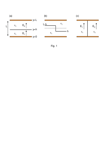
Figure 1: Two liquids in uniform electric field. (a) Schematic illustration of two liquids with permittivities $\varepsilon_{1}$ and $\varepsilon_{2}$ confined between two plates at separation $L$ and voltage difference $V$. The pressure on the interface located at $y=h$ is given by Eq. (9). (b) An initially flat interface at $h=L/2$ can break into two parts. The electrostatic energy, given by Eq. (10), prefers $h=0$ or $h=L$. The preferred state is shown in (c).

Let us now go a step further in elucidating the role of dielectric interfaces by allowing the flat interface to break into two parts of equal area with heights $h$ and $L-h$, such that the volume of the fluids is conserved [Fig. 1(b)]. For simplicity we assume the initial interface to be at $y=L/2$. We ignore edge effects and use the previous exercise for the electrostatic energy to get

$$\frac{F_{\rm es}(h)}{LS}=-\frac{1}{2}\frac{\varepsilon_{1}\varepsilon_{2}\bar{\varepsilon}E_{0}^{2}}{\varepsilon_{1}\varepsilon_{2}+(h/L)(1-h/L)(\Delta\varepsilon)^{2}}~{}.$$ (10)

Here, $F_{\rm es}$ is symmetric around $h=L/2$, and the analysis shows us that the minimum energy is achieved when $h=0$ ($h=L$ is equivalent). At this state, the fluid interface perpendicular to the field has disappeared and was replaced by an interface parallel to the external field [Fig. 1(c)]. The difference between the initial ($h=L/2$) and final ($h=0$) states is

$$\frac{\Delta F_{\rm es}}{LS}=\frac{1}{2}\frac{(\Delta\varepsilon)^{2}}{\bar{\varepsilon}}E_{0}^{2}~{}.$$ (11)

This important result shows us that (i) dielectric interfaces parallel to the external field are electrostatically favored over perpendicular interfaces and that (ii) the energy difference between the two cases scales like $E_{0}^{2}$ and is proportional to $(\Delta\varepsilon)^{2}$. The deformation of a dielectric drop in electric field is in line with this understanding – by elongating along the field, the drop decreases the area of surface perpendicular to the field compared to the unperturbed sphere.

II.2 The instability in pure dielectric liquids

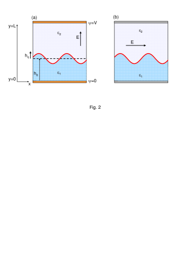
Figure 2: Stabilization and destabilization by electric field. (a) Two liquids in perpendicular electric field. $h_{0}$ is the unperturbed interface location. Interface perturbations are unstable if their wavelength is long enough. (b) A liquid film is stabilized in tangential electric field.

The above derivation leads to the intuitive understanding that there is an electrostatic free energy penalty for dielectric interfaces perpendicular to the external field. Thus, the perpendicular field destabilizes the fluid interface initially parallel to the substrates, as found by Taylor and McEwan (1965) and Melcher and Smith (1969) [Fig. 2(a)]. Melcher also noted that an imposed electric field stabilizes an interface parallel to it Melcher and Schwartz (1968); Onuki (1995b). In the following we present a simplified treatment of the dynamical destabilization process following the lines of Herminghaus (1999) and Schäffer et al. (2000). The main aim is to find how the period and time constant of the pattern evolving in the film depend on the surface tension and electric field.

Consider fluid confined between two parallel and flat electrode separated by a distance $L$ and potential difference $V$, as is schematically depicted in Fig. 2(a). The fluid has dielectric constants $\varepsilon_{1}$ and unperturbed thicknesses $h_{0}$. We consider first the thin-film case, where the gap contains a gas with dielectric constant $\varepsilon_{2}$. Generalization to the bilayer case of two viscous fluids is relatively easy. As a simple approximation, the flow profile is assumed to be Poiseuille-like, and the integrated current along the $y$ direction, $j(x)$, satisfies

$$j(x)=-\frac{h^{3}}{3\eta}\frac{\partial p}{\partial x}~{},$$ (12)

where $\eta$ is the liquid viscosity and $x$ is the direction parallel to the interface.

There are three different contributions to the pressure on the film $p$: the first one comes from the interfacial tension $\gamma$ between the two fluids, $p_{\rm int}=-\gamma h^{\prime\prime}(x)$. The second contribution is electrostatic, as given by Eq. (9). For thin enough films, van der Waals forces come into play, giving rise to a disjoining pressure $p_{dis}=A/6h^{3}$, where $A$ is the Hamaker constant. For thin liquid films, gravity may be neglected; however, gravity effects may easily be incorporated Onuki (1995b).

One may consider perturbations of the flat interface $h(x)=h_{0}+\delta h(x,t)$, where $\delta h\ll h_{0}$. The linear stability analysis will be restricted to the long wavelength limit, $\delta h^{\prime}(x)\ll 1$. We may thus expand $p_{\rm es}$ and $p_{\rm dis}$ to linear order in $\delta h/h_{0}$ to obtain

$$p(x)\simeq-\gamma\delta h^{\prime\prime}-\frac{A}{2h_{0}^{4}}\delta h-\frac{\varepsilon_{1}\varepsilon_{2}(\Delta\varepsilon)^{2}E_{0}^{2}}{L\left(\varepsilon_{1}+h_{0}\Delta\varepsilon/L\right)^{3}}\delta h+{\rm const.}$$ (13)

This expression for the pressure, together with Eq. (12), is used in the continuity equation $\partial h/\partial t+\partial j/\partial x=0$. We look at surface waves of the form $\delta h(x,t)=h_{q}e^{t/\tau}\cos(qx)$, where $\tau$ is the characteristic exponential time for the modulation with wave number $q$ and $h_{q}$ is the amplitude. The dispersion relation between $\tau$ and $q$ is readily obtained to be Schäffer et al. (2001)

$$\frac{1}{\tau}=\frac{\gamma h_{0}^{3}}{3\eta}q^{2}\left(\xi_{e}^{-2}-q^{2}\right)~{}.$$ (14)

The generalized “healing length” is defined by the relation

$$\xi_{e}^{-2}=\frac{A}{2\gamma h_{0}^{4}}+\frac{\varepsilon_{1}\varepsilon_{2}(\Delta\varepsilon)^{2}E_{0}^{2}}{\gamma L\left(\varepsilon_{1}+h_{0}\Delta\varepsilon/L\right)^{3}}~{}.$$ (15)

A positive $\tau$ means the modulation $\delta h(x,t)$ grows in time; negative $\tau$ shows exponential decay. Clearly, all $q$’s smaller than $\xi_{e}^{-1}$ are unstable. $\tau$ is infinite when $q\to 0$ since liquid must then be transported to very long distances; the opposite limit, $q\to\infty$, is also reasonable because very short wavelengths are rapidly attenuated due to surface tension.

The fastest-growing mode $q^{*}$ is given by $q^{*}=\xi_{e}^{-1}/\sqrt{2}$. Since $A\sim 10^{-20}$ J, films thicker than few nanometers are dominated by the electrostatic forces even at moderate field strengths $E_{0}$. If the dispersive part can be neglected, we find that the wavelength of the fastest-growing wave $\lambda^{*}$ is

$$\lambda^{*}=2\pi/q^{*}\sim\gamma^{1/2}/\Delta\varepsilon E_{0}~{}.$$ (16)

Thus, the most unstable wavelength can be reduced by increasing the dielectric contrast $\Delta\varepsilon$ or the field or by decreasing the surface tension between the two liquids $\gamma$.

This normal-field instability also occurs in bilayers of two viscous liquids. A straightforward generalization Lin et al. (2001) gives the same expression as in Eq. (14), only with the viscosity $\eta$ replaced by a rather complicated function of the two liquid viscosities, $C(\eta_{1},\eta_{2})$. The time scale of the dynamics is accelerated by as much as $~{}50$ times, while $q^{*}$ and $\lambda^{*}$ stay intact. The main advantage is the possibility to use liquid pairs with small interfacial tension, thereby reducing $\lambda^{*}$.

II.3 Experiments

Initial experiments were conducted on thin polymer films above the glass transition temperature, with electrode gap $L<1~{}\mu$m. In addition to the basic understanding of interfacial phenomena in electric fields, experiments were motivated by the possibility of a new lithography technique Chou and Zhuang (1999). Indeed, amplification of the most unstable mode leads to a film with a well-defined periodicity.

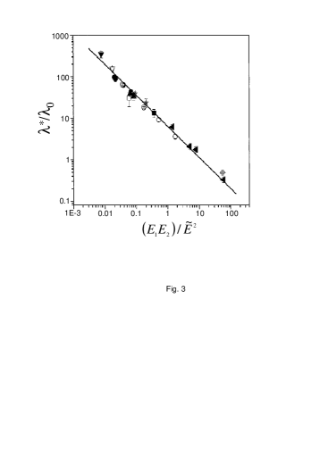
Figure 3: Plot of the most unstable wavelength $\lambda^{*}$ vs reduced electric field for various thin films. $E_{1}$ and $E_{2}$ are the electric fields in the two liquids, $\lambda_{0}=V^{2}(\Delta\varepsilon)^{2}/\gamma(\varepsilon_{1}\varepsilon_{2})^{1/2}$, and $\tilde{E}=V/\lambda_{0}$. The expected relation from Eq. (16), $\lambda^{*}/\lambda_{0}=2\pi(E_{1}E_{2}/\tilde{E}^{2})^{-3/4}$, is the straight line with slope of $-3/4$. Adapted with permission from Lin et al. (2002). Copyright 2002 American Chemical society.

Figure 3 shows a plot of $\lambda^{*}$ for a series of experiments with different parameters: liquid thickness $h_{0}$, spacing $L$, voltage $V$, etc. The plot shows a good agreement with Eq. (16) when the axes are suitably defined Lin et al. (2001). For a summary of data from several groups, the reader is referred to Pease and Russel (2003).

Hierarchical hexagonal structures have been obtained in sophisticated experiments by the use of a trilayer, namely, a liquid-liquid-air sandwich Morariu et al. (2003). The resulting structures have two different periodicities, depending on the dynamical process and on the relative volumes of the components.

II.3.1 Topographic electrodes

With smooth electrodes, the pattern period $\lambda^{*}$ [Eq. (16)] depends on the electric field, interfacial tension, and dielectric contrast. For technologically motivated reasons, it may be beneficial to achieve different patterns. The use of a topographically patterned electrode enables facile and rapid duplication of a “master mask” onto the liquid film Schäffer et al. (2000) since the interfacial instability is amplified in places where the electrode gap is smaller. Figure 4 shows an implementation of this idea. Subsequent quench freezes the structure.

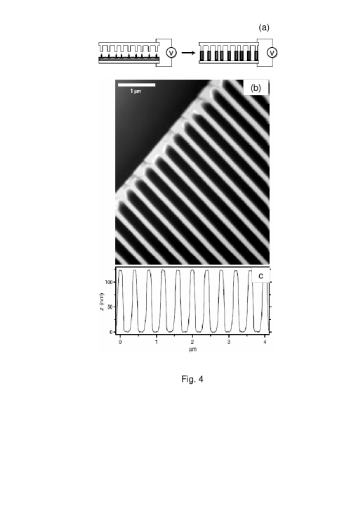
Figure 4: Pattern transfer. Use of topographically patterned electrodes enables transfer of the top electrode onto the polymer liquid, as is depicted schematically in (a). Tapping-mode atomic force microscopy images in (b) and (c) show the resulting topography of the polymer layer. Adapted by permission from Macmillan Publishers Ltd: Schäffer et al. (2000).

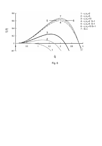
Figure 5: Dispersion relation between wave number [scaled by $(\varepsilon_{2}V^{2}/\gamma L^{3})^{1/2}$] and inverse growth time [scaled by $\eta_{1}\gamma L^{3}/\varepsilon_{2}^{2}V^{4}$]. Curves 1–3 are for pure dielectric liquids, Eq. (14). Curves 4–6 are from the “leaky dielectric” model with small dimensionless conductivity $S$. The conductivity in curve 7 is infinite. Reprinted from Pease and Russel (2002), Copyright (2002), with permission from Elsevier.

II.3.2 Residual conductivity

Work with polymer pairs gives smaller $\lambda^{*}$ because of the reduced surface tension, but at the same time the dielectric contrast $\Delta\varepsilon$ is diminished. How can this deficiency be overcome? We must return to the role of residual conductivity in polymers. Conductivity difference between two layered liquids leads to charge accumulations in interfacial regions and to additional interfacial stress.

Pease and Russel (2002) studied the application of Taylor’s leaky dielectric model to this system. Their analysis for slightly conductive polymer films yielded growth exponents and characteristic wave numbers much larger than that of perfect dielectrics: even very small conductivities decrease the growth exponent $\tau$ markedly and decrease the fastest-growing wavelength $\lambda^{*}$ by a factor of $2$–$4$. This is shown in Fig. 5, where $q$ and $\tau$ have been appropriately scaled. The dimensionless conductivity $S$ is defined by $S=\eta_{2}\gamma\sigma L^{3}/\varepsilon_{2}^{3}V^{3}$, where $\sigma$ is the conductivity. The numerical value of $S$ greatly varies and can be between $0.1$ and $10^{16}$. Note that according to the model, small conductivity has a drastic effect on the dispersion relation and that changing from $S\ll 1$ to $S>1$ does not change much.

II.4 Near-critical fluids

It is in order to briefly mention here near-critical fluids. The two fluids described above may be a liquid in coexistence with its vapor phase or a binary mixture of two partially miscible liquids. If one approaches the critical point from below, $T\to T_{c}$, the surface tension and the dielectric contrast vanish like $\gamma\simeq\gamma_{0}(1-T/T_{c})^{2\nu}$ and $\varepsilon_{2}-\varepsilon_{1}\propto(T_{c}-T)^{\beta}$, where $\nu\simeq 0.625$ and $\beta\simeq 0.33$ are the exponents characterizing the correlation length and the liquid-vapor density difference (zero-field magnetization in magnetic systems). As Onuki (1995b) pointed out, this implies that $\lambda^{*}$ can be reduced upon approach to $T_{c}$ as

$$\lambda^{*}\sim\gamma^{1/2}/\Delta\varepsilon\sim(T_{c}-T)^{0.295}~{}.$$ (17)

The relaxation dynamics of our simple model is influenced by the vanishing of $\gamma$ as $T_{c}$ is approached and is different in the short- or long-wavelength limits. One should bear in mind, though, that the derivation used above breaks down in this limit since we have used the assumption of sharp interfaces between the liquids. The model is valid as long as the interfacial width between the liquids $w\sim(T_{c}-T)^{-1/2}$ is much smaller than the unstable wavelength: $w\ll\lambda^{*}$.

II.5 Other related instabilities

It is useful to mention several related instabilities originating from electric fields. Andelman et al. (1986) considered a Langmuir monolayer of polar molecules. These dipoles are constrained to the interface between two fluids, typically water and air, pointing in a direction perpendicular to the interface. Since parallel dipoles repel each other, their concentration may show modulations. On writing the dipole surface density as $n(x)=n_{0}+n_{q}e^{iqx}$, they found the electrostatic energy of the dipoles per unit area to be $F_{\rm es}=-(1/2)|q|\varepsilon_{2}/[\varepsilon_{1}(\varepsilon_{1}+\varepsilon_{2})]d^{2}n_{q}^{2}$. Here $d$ is the electric dipole moment of individual molecules. The electrostatic energy thus prefers a modulated state with infinitesimal period. The system is unconstrained in the direction perpendicular to the two liquids, hence the $-|q|$ dependence. The competition between the long-range dipole-dipole repulsion and interfacial tension between “phases”, scaling as $q^{2}$, leads to an unstable mode with finite wavelength McConnell et al. (1984). The simple analytical model, valid in the long-wavelength limit, enabled them to construct a phase diagram of modulated phases with hexagonal and stripe symmetries Andelman et al. (1987). Similar behavior was found by Garel and Doniach (1982) for thin uniaxial ferromagnetic slabs subject to a perpendicular magnetic field even though the physical origin of the dipoles is different in the two cases. Another system of interest consists of a charged end-group polymer brush placed inside a parallel-plate condenser. The electrostatic energy per unit area associated with end-group height undulation of the form $h(x)=h_{0}+h_{q}\cos(qx)$ can be written to quadratic order in $h_{q}$ as $F_{\rm es}=-\sigma^{2}/\varepsilon|q|\cosh(qh_{0})\cosh[q(L-h_{0})]/\sinh(qL)h_{q}^{2}$. Here $\sigma$ is the charge per unit area, $L$ is the surface separation and $\varepsilon$ is the dielectric constant of the uniform embedding medium. One retrieves the $F_{\rm es}\sim-|q|$ dependence in the symmetric case where $h_{0}=L/2$ and in the limit $L\to\infty$ Tsori et al. (2008). Again, the surface is unstable with respect to a finite wavelength. This result essentially recapitulates the studies on the instability appearing in ³He-⁴He interface when it is charged with ions Wanner and Leiderer (1979); Etz et al. (1984). The instability of Sec. II is dynamical because once the interface is parallel to the field, the field stabilizes it. Here, however, the instability appears in equilibrium because due to its charge, the interface is frustrated even if it is perpendicular to the substrate.

In a related work, Du and Srolovitz (2004) considered the stability of the metal electrodes themselves to surface modulations. Two parallel metals with potential difference $V$ and separated by an insulator are commonly found in many situations, such as in micro-electro-mechanical-systems, microswitches, and close to scanning transmission microscopy tips. They used the same long-wavelength approximation and obtained the electrostatic energy $F_{\rm es}=-(1/8)|q|\varepsilon E_{0}^{2}\coth(qL)h_{q}^{2}$, where $h_{q}$ is now the amplitude of electrode surface modulation. When interfacial tension was added, they found that all surface modes with $q<q_{c}$ are unstable, where $q_{c}$ is given by $q_{c}=\varepsilon E_{0}^{2}\coth(q_{c}L)/4\gamma$. However, the system is most unstable with respect to long wavelengths, that is, $q^{*}=0$.

The stability of a poorly conducting lipid membrane in aqueous environments in perpendicular electric field was studied as well Sens and Isambert (2002). The accumulation of charges on the opposite sides of the membrane is unbalanced if the membrane is not completely flat. The destabilizing electric field acts like a negative surface tension, tending to enlarge the membrane area. For a freely suspended membrane, a hydrodynamic theory gives the fastest-growing $q$ mode $q^{*}\sim(E_{0}R)^{2/3}$, where $E_{0}$ is the external field and $R\simeq 10^{5}$ is the ratio between the membrane and solvent resistivities. The corresponding wavelength is $\lambda^{*}=2\pi/q^{*}\simeq 0.5\mu$m and the growth rate is $\tau\simeq 10^{5}-10^{6}$ s^-1.

Lastly, we mention the normal-field instability in ferrofluids, an important phenomenon discovered by Cowley and Rosensweig (1967). When the interface between a ferrofluid and a nonmagnetic fluid is subject to a perpendicular magnetic field, the surface becomes unstable if the magnetization exceeds the critical value, $M_{c}$. The static pattern is hexagonal, and its period $\lambda^{*}$ is given by $\lambda^{*}=2\pi(\gamma/g\Delta\rho)^{1/2}$ Rosensweig (1997); Andelman and Rosensweig (2009).

II.6 Immiscible liquids in electric fields: Electrowetting

Until now, we have described (i) how an initially flat liquid layer becomes unstable under the influence of a perpendicular electric field and (ii) the deformation of a liquid drop in external fields. We now briefly describe an “intermediate” situation, that of a liquid drop placed on a solid flat substrate in electric field. Classical electrowetting describes the change in the wetting properties of two immiscible liquids due to the field Mugele and Baret (2005). This is a broad topic with many important applications in microfuidics, lab-on-a-chip, etc. Stone et al. (2004).

Consider first a dielectric drop embedded in a dielectric medium. For simplicity, we assume dc voltage and steady-state situation. The elongation of dielectric drops not in contact with any substrate, as considered by O’Konski and Thacher [see Eq. (6)], may lead us to think that drop will elongate in the field’s direction, thereby reducing the contact area with the substrate and increasing the contact angle. The general shape change is correct, but at the contact line this intuition fails: the contact angle $\theta$ stays the same. The reason that $\theta$ is independent of $E_{0}$ is because the electrostatic energy scales as the volume while the interfacial energies scale as the area. Upon looking at ever smaller regions close to the three-phase contact line, we thus find that the electrostatic force becomes negligible compared to the interfacial forces. The apparent contact angle, measured at a macroscopic scale, may be larger than the field-free angle.

For a conducting drop, the situation is very different: charge accumulation at a very thin layer at the substrate means the energy contribution of the electric field becomes proportional to the surface and not to the volume. This leads to a modification of the interfacial properties and hence the apparent wetting angle changes from $\theta$ to $\theta^{*}$. The main differences from Taylor’s work on weakly conducting drops are (i) the existence of a solid surface and the localization of electric field at it and (ii) the embedding medium, usually a vapor, is nonconducting.

Lippmann’s original work on electrolytes asserted that the solid-vapor interfacial tension $\gamma_{\rm sv}$ is unaffected by the potential, but solid-liquid interfacial tension $\gamma_{\rm sl}$ is reduced by a value proportional to $V^{2}$ Lippmann (1875). This reduction is due to the spontaneous creation of an electric double layer at the substrate. However, in the cases where the electrode is metal, electrolysis usually makes it difficult to achieve high voltages. It is therefore beneficial to cover the electrode with a dielectric insulator of thickness $d$ and permittivity $\varepsilon$. In this situation, the dielectric is responsible for the system’s capacitance, and the effective solid-liquid interfacial tension $\gamma_{\rm sl}^{*}$ is given by Berge (1993),

$$\gamma_{\rm sl}^{*}\simeq\gamma_{\rm sl}-\frac{\varepsilon}{2d}V^{2}~{}.$$ (18)

The apparent contact angle $\theta^{*}$ is found from substitution of $\gamma_{\rm sl}^{*}$ in Young’s equation and is given by

$$\cos\theta^{*}=\cos\theta+\frac{\varepsilon(V-V_{0})^{2}}{2\gamma d}~{}.$$ (19)

The $V_{0}$ term accounts for spontaneous charging – it is common that a solid in contact with an electrolyte inherits a net charge by ion adsorption or ionization of covalently bound groups. For instance, common glass near water ionizes to make SiO^- and releases a proton. The above supposes a wedge-shaped interface and is correct on a macroscopic scale. On a scale smaller than thickness of the dielectric layer $d$, the curvature of the liquid-vapor interface is not fixed.

In the absence of a disjoining pressure, the interface shape is governed by the generalized Laplace’s equation,

$$\gamma\kappa({\bf r})-p_{\rm es}({\bf r})={\rm const.}$$ (20)

Here $\kappa$ is the local curvature and $p_{\rm es}\propto V^{2}$ is the electrostatic pressure, calculated globally for the drop Mugele and Baret (2005). At the mesoscopic scale, a numerical procedure assuming a circular contact line showed that the electric field diverges weakly at the three-phase contact line, and the slope approaches Young’s angle, $\theta$, at the contact line Buehrle et al. (2003); Bienia et al. (2006). This theoretical finding has been verified experimentally recently Mugele and Buehrle (2007). Note that the drop’s shape needs not stay circular, and a static instability of the contact line was observed in high voltages Mugele and Herminghaus (2002). In contrast to the instability discussed throughout Sec. II, here the complex interfacial shapes are static due to a balance between Laplace and electrostatic pressures.

The influence of time-varying ac fields depends on the field’s frequency $\omega$: for a liquid drop of dielectric constant $\varepsilon$ and conductivity $\sigma$, the drop behaves as in dc field if it is in the quasistatic regime, that is, when $\omega\ll\omega_{c}$ Landau et al. (1984); Mugele and Baret (2005), where

$$w_{c}=\sigma/\varepsilon~{}.$$ (21)

In the opposite regime, $\omega\gg\omega_{c}$, the mobile ions do not have enough time to response to the field before it changes sign. Electric double layer is not created, and therefore the field acts throughout the whole drop volume. The electric field thus exerts a body volume force again just like for static dc fields in pure dielectrics. Experimentally, demineralized water have $\sigma\simeq 4\times 10^{-6}$ S m^-1 and therefore at frequencies $\omega>10^{4}$ s^-1 the behavior is similar to the dielectric case. The frequency $\omega_{c}$ appears also as an important measure of the influence of ions on orientation of block copolymers by electric fields (see Sec. III.5).

As a final comment, we stress that all of the above is not valid close to a critical point: if $T-T_{c}$ is small enough, the correlation length diverges, and the interfacial tensions $\gamma$, $\gamma_{\rm sv}$, and $\gamma_{\rm sl}$ become dependent on the field distribution and droplet shape.

III Block-Copolymer Orientation in Uniform Electric Fields

The preceding section described several examples of deformation of an interface between two immiscible liquids or between a liquid in coexistence with its vapor. In both cases the two phases are macroscopic, separated by a thin interfacial layer. An interesting question regards the effect of electric field on complex materials which self-assemble into ordered structures with typical lengths on the mesoscopic scale. We will concentrate on one such material – block copolymers (BCPs). These consist of two or more chemically distinct polymer species connected by a covalent bond. Their self-assembly results from a competition between enthalpic interactions and chain stretching of entropic origin Bates and Fredrickson (1999). Block copolymers have attracted considerable research in the past years because many of their interesting mechanical, electrical, rheological, and other properties can easily be fine tuned for optimum performance in nanotechnological applications Park et al. (2003).

The phase behavior of diblock copolymers, made up of two polymers A and B, is governed by two parameters: $\phi_{0}$, the volume fraction of the A polymer ($0<\phi_{0}<1$) and $N\chi$. $\chi$ is the so-called Flory parameter and is approximately inversely proportional to the temperature and $N$ is the polymerization index. In symmetric diblock copolymers, the A and B parts of the polymer have the same length, and $\phi_{0}=1/2$. If the temperature is high enough (small $N\chi$), the melt is found in a disordered phase. Cooling below the so-called order-disorder temperature (ODT) leads to the appearance of a lamellar phase. This is a one-dimensional and periodic phase of A- and B-rich domains of width $d$ comparable to the polymer radius of gyration. At fixed temperature, further increase in the length asymmetry between the A and B blocks (larger $|\phi_{0}-1/2|$) increases the spontaneous curvature: the polymers adopt a configuration where the shorter block is confined to the inside of cylinders arranged on a hexagonal lattice. Even larger increase in $|\phi_{0}-1/2|$ leads to the formation of spheres arranged on a bcc phase. Other more complicated ordered phases appear in block copolymers and even in simple diblocks (e. g., gyroid phase), but we ignore them here. The region in the phase diagram in the $(\phi_{0},N\chi)$ plane close to the ODT point, given by $N\chi\simeq 10.5$, is called the weak-segregation regime. In this region, domain spacing $d$ scales like $N^{1/2}$. The region farther below the ODT point, $N\chi\gg 10.5$, is called the strong-segregation regime, where the A and B blocks are highly segregated from each other, and $d\sim N^{2/3}$.

III.1 Orientation mechanism

The orientation of block copolymers and indeed many other soft-matter phases can be influenced by several external fields. Examples are shear flow, van der Waals or chemical interaction with surfaces, confinement by walls, etc. At first inspection, it seems that electric fields are very weak since the electrostatic energy stored in a molecular volume $v_{0}$, $v_{0}\varepsilon E^{2}$, is much smaller than the thermal energy $k_{B}T$. However, experiments have shown that this estimate is too simplistic and $v_{0}$ is not the relevant volume. The first experiments on block copolymers in electric fields were carried out by Amundson et al. (1991). In a series of papers they developed the key concepts for alignment and stability of lamellar phases in electric fields Amundson et al. (1993, 1994). In the first set of experiments, polystyrene-polymethylmethacrylate (PS/PMMA) was anionically synthesized. Samples were heated above the ODT point, held for about 10 min, and then cooled below the ODT in the weak-segregation region. In the absence of an electric field, a small-angle x-ray scattering (SAXS) reveals a characteristic ring, corresponding to a repeat period of $d=23$ nm. Samples under electric field, however, exhibit strong anisotropy, as is manifest in the clear peaks appearing in the direction perpendicular to the electric field.

Figure 6: Orientation of PS/PMMA block copolymer lamellae. (a) The bulk experiments of Amundson et al. (1993) show near-perfect alignment of lamellae in the direction parallel to the external field. (b) Time evolution of the orientational order parameter $S$ for two samples with different cooling rates as measured by birefringence experiments. Solid line is an exponential fit. Adapted with permission from Amundson et al. (1993). Copyright 2002 American Chemical society. (c) TEM closeup of cylindrical diblock copolymers near an electrode. Inset is schematic illustration of the full setup. Dashed arrows are field lines and box indicates area of image. Note how cylinders curve and follow the field lines near the corner. From Morkved et al. (1996). Reprinted with permission from AAAS.

Figure 6(a) is a transmission electron micrograph (TEM) of lamellae oriented in electric field. In order to quantify the alignment of ordered phases, Amundson et al. (1993) used the quantity $S$ defined as follows. Denote by $\phi({\bf r})$ the local A-polymer composition ($0<\phi<1$). In the disordered phase, $\phi$ is equal to its average value $\phi_{0}$. One can write $\phi({\bf r})$ as a sum of plane waves of the form

$$\phi({\bf r}) = \phi_{0}+\varphi({\bf r})~{},$$

$$\varphi({\bf r}) = \sum_{{\bf q}\neq 0}\varphi_{\bf q}e^{i{\bf q}\cdot{\bf r}}~{}.$$ (22)

For example, close to the ODT point, a lamellar phase can be described by $\phi({\bf r})=\phi_{0}+\varphi_{L}\cos(qx)$, where $\varphi_{L}$ is an amplitude and the normal to the lamellae is chosen in the $x$ direction. Similarly, hexagonal and cubic phases contain three and six modes, respectively. For a lamellar phase, the average orientation $S$ is then defined by

$$S=\frac{3}{2}\langle(\hat{q}\cdot\hat{E}_{0})^{2}\rangle-\frac{1}{2}~{}.$$ (23)

In nematic liquid crystals, $S$ is commonly used to quantify order. In the beginning of the process, there are many random grains in different directions not correlated with the field, the sample is macroscopically disordered, and therefore $S=0$. As orientation of lamellar grains proceeds, ${\bf q}$ turns until it becomes perpendicular to ${\bf E}_{0}$ for reasons which will become clear below. Perfect orientation has $S=-1/2$. Figure 6(b) is a time-evolution plot of $S(t)$. The evolution is slow because the samples are very viscous. The sample with slow cooling rate equilibrates faster to the electrostatically preferred orientation. Figure 6(c) is a TEM image taken by Morkved et al. (1996) close to the electrodes. Clearly, lamellae seem to follow the curved field lines.

III.2 Experiments

The recent decade has witnessed an explosion of work on electric-field effects in block copolymers. Experiments can be roughly divided to two types: those carried out in a block copolymer melt and those in a solution. In the first case, pure block copolymer melt is subject to an external electric field. Since the melt is very viscous, the sample is heated to elevated temperatures and subsequently annealed under electric field. SAXS, TEM, and small-angle neutron scattering are used to characterize the copolymer structures. Annealing times are very long, and therefore experiments in copolymer melts intrinsically probe static phases. On the other hand, when copolymers are dissolved in a solvent, the viscosity is not high and orientation kinetics in electric field can be recorded.

III.2.1 Statics

The experiments of Amundson et al. (1994) showed that block copolymer structures can be oriented in the bulk. This work has stimulated further attempts to orient thin film structures. The advantage in using thin films is their possible technological applications and the reduction in required voltage following the reduction in size. The disadvantage in size reduction is that the electric field, acting throughout the sample volume, needs to overcome increasingly more dominant interfacial energies acting between the copolymers and the bounding surfaces.

The experiment in Fig. 6(c) and others Mansky et al. (1998) showed that BCP domains can be oriented laterally along an external field even in a thin film. Consider a BCP melt sandwiched between two flat and parallel surfaces at distance $L$ from each other and potential difference $V$. One would naively expect that there is one transition field, below which BCP lamellae (or cylinders) are parallel to the substrate and above which domains are perpendicular to it. The electric field acts throughout the sample volume, and therefore the order of magnitude of field strength required for effective orientation is given by $\varepsilon E^{2}\sim\gamma/L$, where $\gamma$ and $\varepsilon$ are the typical difference between the interfacial tensions of the polymers with the substrate and dielectric constant. In most experimental systems $\gamma\sim 10$-$100$mN, $L\sim 10$-$100~{}\mu$m, and $\varepsilon\sim 5\varepsilon_{0}$, and we therefore find $E\sim 10^{3}$-$10^{7}$ V/m. The larger value of these estimates is quite a large field, but it is nonetheless considerably smaller than the dielectric breakdown threshold, $E\sim 10^{8}$ V/m.

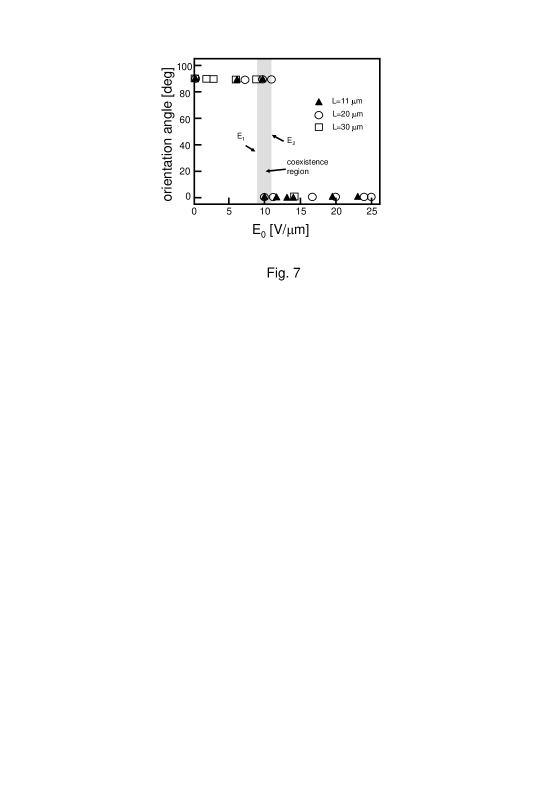
Figure 7: Summary of sample orientation with respect to the field. Orientation angle is the angle between cylinders’ axis and external field for three different film thicknesses $L$. Shaded area is a coexistence “mixed” region, where both orientations are observed. Critical fields $E_{1}$ and $E_{2}$ mark the transition fields between the three possible states (cylinders parallel or perpendicular to the surface and a mixed state). Adapted with permission from Thurn-Albrecht et al. (2000). Copyright 2002 American Chemical society.

Subsequent work on BCP thin films verified that electric field can indeed orient lamellae and cylinders from a direction parallel to the substrate to a direction perpendicular to it (and parallel to the field) Thurn-Albrecht et al. (2000). Anionically synthesized samples of PS/PMMA in the disordered (high temperature) state were exposed to electric fields of $1$–$25$ V/$\mu$m. One aluminum electrode was in direct contact with the copolymers, while the second one was insulated from the copolymers by a Kapton sheet. The sample was then cooled down to the cylindrical phase and held for 14 h, and finally cooled to room temperature. SAXS experiments, shown on Fig. 7, revealed the following general picture: surprisingly, there are two critical fields $E_{1}$ and $E_{2}$. If $E<E_{1}$, cylinders are parallel to the substrate, while above $E_{1}$ they are destabilized. If $E_{1}<E<E_{2}$, there is a mixed state, showing characteristics of both parallel and perpendicular cylinders. If $E>E_{2}$, the sample is fully oriented perpendicular to the substrate and parallel to the external field.

As mentioned above, due to the high polymer viscosity, experiments in the melt can be performed with polymers of limited molecular weight. Typically, large electric fields are required in order to overcome defects that persist in the sample and to accelerate the slow dynamical process. A different approach was presented by Böker et al. (2002), whereby copolymers are dissolved in a solvent. The use of a polymer solvent allows additional experimental flexibility: for example, a selective solvent for one of the polymers may, in principle, effectively increase the dielectric contrast $\Delta\varepsilon$, and it also enables use of high molecular weight and branched polymers. In addition, because the solution is less viscous than the melt, the full orientation kinetics can be recorded in real time. However, a usual deficiency of this approach is the nonselectivity of common solvents: as the solvent dissolves in the respective polymer blocks, the effective dielectric contrast $\Delta\varepsilon$ between domains is diminished.

Bulk samples of polystyrene-poly(2hydroxyethyl methacrylate)-polymethylmethacrylate (PS/PHEMA/PMMA) with number-average molecular weight M_n of 82 000 g/mol were dissolved in chloroform and put in a cylindrical capacitor with average electric field $E_{0}=1.8$ V/$\mu$m. The solvent evaporated in a controlled manner and under the influence of external field, and the resulting samples were characterized by SAXS, TEM, and differential scanning calorimetry. These techniques show that the PHEMA block is miscible with the PMMA block and that the triblock copolymer actually behaves very similar to a PS/PMMA diblock of enhanced dielectric contrast. The experiments showed that block-copolymer solutions can be efficiently oriented parallel to the external field, overcoming interfacial interactions. In addition, they also opened a window for quantitative consideration of defect statistics and, more importantly, the dynamics of grain orientation and defect annihilation.

III.2.2 Dynamics

As is explained above, one of the advantages of orientation in polymer solutions is the possibility to track orientation dynamics. In order to record dynamics, a high-flux scattering source is required because the exposure time is limited as compared to static experiments. Another important consideration is the copolymer volume fraction in solution: less copolymer not only reduces the viscosity but also reduces the effective dielectric contrast $\Delta\varepsilon$. The electric field needs to be high enough so that orientation terminates before solvent evaporation completes and the structure becomes virtually immobile. Böker et al. (2003) used lamellar-forming polystyrene-polyisoprene (PS/PI) block copolymer dissolved in toluene. The samples were exposed to synchrotron SAXS of high beam energy and photon flux during exposure to electric field. The synchrotron beam direction was perpendicular to the electric field’s direction. The measured average sample orientation, as indicated by $S(t)$ of Eq. (23), showed a similar qualitative behavior as in Fig. 6(b). But there is a big difference – the dynamics are 20-fold faster. The relaxation of $S(t)$ is characterized by a single exponential with time constant $\tau$. As expected, $\tau$ increases with increasing copolymer content and decreasing temperature.

Using in situ SAXS experiments, Böker et al. (2003) identified two mechanisms for orientation of ordered phases: close to the ODT point, the polymer solution undergoes a transition between only two orientations (from perpendicular to parallel to ${\bf E}_{0}$), with no intermediate orientations. Grains of lamellae in the favorable direction grow on the expense of unfavorable grains, resulting in grain boundary migration. However, far from the ODT point (lower temperatures), the scattering pattern has all the intermediate grain orientations and thus reflects continuous rotation of grains to the favorable direction. The optimum grain orientation is not fully achieved since the driving force for orientation, torque, is negligibly small at long times.

What is the nature of the “driving force”? Figure 8 shows the collection of results from numerous systems with different copolymer solutions. For all four copolymer solutions, the inverse exponential relaxation time $\tau^{-1}$ scales linearly with $E_{0}^{2.7}$, with scaling prefactor depending on the specific solution. The exponent, being $2.7$ and not $2$, is attributed to alignment process governed by an energy barrier; this is a feasible explanation in the weak-segregation regime, where grain orientation is dominated by nucleation and growth Schmidt et al. (2007). A simple scaling form exists validating the importance of the dielectric contrast $\Delta\varepsilon$: when the data are presented for $\eta/\tau$ against $(\Delta\varepsilon)^{2}E_{0}^{2}/\bar{\varepsilon}$, where $\eta$ is the solution viscosity, all data except one collapse onto a universal curve.

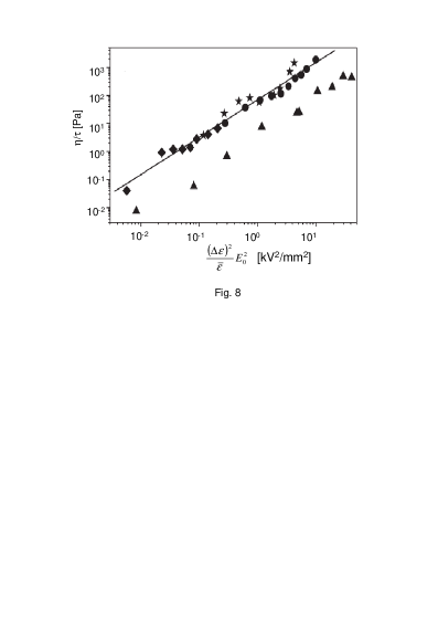
Figure 8: Inverse exponential relaxation time $\eta/\tau$ against $E_{0}^{2}$ from four copolymer solutions as obtained by SAXS. When properly scaled, most data sets fall on a single universal curve. From Schmidt et al. (2007). Reproduced by permission of The Royal Society of Chemistry.

A general theory of orientation of ordered phases is presented below based on a coarse-grained simplified approach.

III.3 Theory

The underlying physical mechanism of copolymer orientation, sometimes referred to as the “dielectric interfaces,” is described below. This mechanism relies on dielectric contrast between the different material domains. The electric field favors one sample orientation over another, the energy difference being proportional to $(\Delta\varepsilon)^{2}E_{0}^{2}$. Intuitively, we may say that there is a free energy penalty for having dielectric interfaces perpendicular to the field’s direction. This is true in both the weak- and strong-segregation regimes, but the analytical theory is different in the two cases.

III.3.1 Electrostatics of strongly segregated lamellae

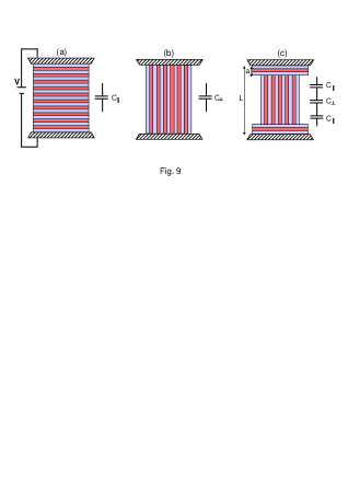
Figure 9: Capacitor analogy for three competing lamellar structures confined in a condenser. (a) Parallel and (b) perpendicular layering and (c) mixed morphology, consisting of two parallel layers of thickness $a$ at the electrodes and perpendicular lamellae throughout the rest of the film. The equivalent electrical circuits are illustrated on the left.

All interesting effects reviewed here are due to dielectric anisotropy. One obvious anisotropy in $\varepsilon$ is due to the mesoscopic order, in which $\varepsilon$ is a function of ${\bf r}$. Another contribution may come from the inherent anisotropy of $\varepsilon$ in the presence of electric field. Indeed, since polymers are large objects with many chemically differing regions, $\varepsilon$ in general is a tensor, and therefore the dielectric response is anisotropic in nature. Here we ignore the tensorial nature of $\varepsilon$ since it is not observed in most experiments. The interested reader may turn to the theoretical description of block copolymers with anisotropic $\varepsilon$ given by Gurovich (1994, 1995).

Strongly segregated lamellae are characterized by a square-wave composition profile $\phi$. For the electrostatic calculation it is therefore reasonable to take lamellae as being composed of pure A and pure B polymers, with dielectric constants $\varepsilon_{1}$ and $\varepsilon_{2}$, respectively, separated by a sharp interface. The capacitor model allows the calculation of electrostatic energy of competing orientations Pereira and Williams (1999); Tsori and Andelman (2002). Consider a stack of lamellae parallel to the electrodes separated by distance $L$ and potential difference $V$, as illustrated in Fig. 9(a). Such parallel lamellae may be stabilized by preferential interactions with the substrate. For symmetric lamellae, we use the continuity of the displacement field $D=\varepsilon E$ across dielectric interfaces and the total potential drop and find the electrostatic energy per unit area to be $F_{\rm es}^{\parallel}=-\frac{1}{2}C_{\parallel}V^{2}$, where the capacitance per unit area $C_{\parallel}$ is given by

$$C_{\parallel}=\frac{\varepsilon_{1}\varepsilon_{2}}{\bar{\varepsilon}}\frac{1}{L}~{}.$$ (24)

Here $\bar{\varepsilon}=(\varepsilon_{1}+\varepsilon_{2})/2$ is the average dielectric constant. Similarly, for the perpendicular arrangement [Fig. 9(b)] we have $F_{\rm es}^{\perp}=-\frac{1}{2}C_{\perp}V^{2}$ and

$$C_{\perp}=\frac{\bar{\varepsilon}}{L}~{}.$$ (25)

Since $C_{\perp}$ is larger than $C_{\parallel}$, the electrostatic energy $F_{\rm es}$ is always lower for the perpendicular lamellae, with the difference between the two orientations being proportional to $(\Delta\varepsilon)^{2}$. Which of the two phases, parallel or perpendicular lamellae, is thermodynamically stable that is a matter of a competition between the interfacial energies, scaling like the substrate area, against the electrostatic energy, scaling like the sample volume. It is clear that there is a critical voltage above which perpendicular lamellae will be preferred over parallel ones. This voltage depends on $\Delta\varepsilon$, $L$, and the interfacial energies.

The two structures above are not the only conceivable ones. More complex phases, such as the one depicted in Fig. 9(c) may be possible. This mixed morphology presents an interesting compromise: the system keeps few parallel layers at the substrates, thus optimizing interfacial interactions, but has lamellae oriented in the field’s direction in the rest of space, thus minimizing electrostatic energy throughout most of the film. However, there is an energetic penalty per unit area of the film, $\gamma_{{}_{T}}$, for the creation of a “T-junction” defect.

The capacitor model allows us to calculate $F_{\rm es}$ for the mixed state as well. The equivalent electrical circuit is that of two “parallel” capacitors and one “perpendicular” one connected in series. Ignoring edge or “fringe” effects, we may write the capacitance of the mixed morphology by

$$\frac{1}{C_{m}}=\frac{2a}{L}\frac{1}{C_{\parallel}}+\frac{L-2a}{L}\frac{1}{C_{\perp}}~{}.$$ (26)

The factors in front of the inverse capacitances on the right hand side are necessary since the parallel layers only occupy a region of width $a$ (equal to several lamellar widths). It is easy to show that $C_{\parallel}<C_{m}<C_{\perp}$.

The free energies per unit area of the three competing phases are given by

$$F^{\parallel} = Lf_{p}+2\gamma_{{}_{\rm AS}}-\frac{1}{2}C_{\parallel}L^{2}E_{0}^{2}~{},$$ (27)

$$F^{\perp} = Lf_{p}+\gamma_{{}_{\rm AS}}+\gamma_{{}_{\rm BS}}-\frac{1}{2}C_{\perp}L^{2}E_{0}^{2}~{},$$ (28)

$$F^{m} = Lf_{p}+2\gamma_{{}_{\rm AS}}+2\gamma_{{}_{T}}-\frac{1}{2}C_{m}L^{2}E_{0}^{2}~{}.$$ (29)

$f_{p}$ is the polymer free energy per unit volume and includes bending and compression. $\gamma_{{}_{\rm AS}}$ and $\gamma_{{}_{\rm BS}}$ are the A and B interfacial energies with the substrate.

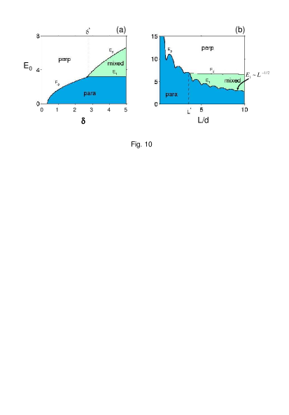
Figure 10: Stability diagrams for confined lamellar phases in the strong segregation regime in electric fields. (a) $L=10d$ and is fixed. Small value of $E_{0}$ leads to parallel layers. Increase in $E_{0}$ leads to a direct transition to perpendicular layers when $\delta=(\gamma_{{}_{\rm BS}}-\gamma_{{}_{\rm AS}})/\gamma_{{}_{T}}$ is small enough. If $\delta$ is large, $\delta>\delta^{*}$, increase in the field induces first a transition to a mixed phase and subsequently to a perpendicular orientation. (b) Diagram in the $E_{0}$-$L$ plane with fixed $\delta=5$. $E_{0}$ is scaled by $(\gamma_{{}_{T}}/d)^{1/2}$. Adapted with permission from Tsori and Andelman (2002). Copyright 2002 American Chemical society.

The minimal model above allows the calculation of phase diagrams as a function of $E_{0}$, $\gamma_{{}_{\rm BS}}-\gamma_{{}_{\rm AS}}$, and $L$. Figure 10 shows two such cuts in the three-dimensional phase space. The transition fields $E_{1}$, $E_{2}$ and $E_{3}$ are lines where the free energies are equal to each other. In part (b), the transition field $E_{1}$, above which parallel lamellae become unstable, has undulations. These are due to the incommensurability between the lamellar period and the film thickness, causing polymer stretching or compression. $E_{1}$ decays like $L^{-1/2}$  – this is easily understood since the interfacial energy is proportional to the area, while the electrostatic energy scales as area $\times LE_{0}^{2}$. $E_{2}$ is the transition field between mixed and perpendicular lamellae and is virtually independent of film thickness $L$. Note that $|\gamma_{{}_{BS}}-\gamma_{{}_{AS}}|$ may be so large that $E_{2}$ is above the threshold for dielectric breakdown ($\sim 150$ V/$\mu$m). In these circumstances perfect perpendicular lamellae throughout the whole film are not possible.

Experiments validate the existence of a mixed morphology. Fig. 11 shows lamellae sandwiched in a thin film in the presence of a perpendicular electric field. Clearly, the film’s center has lamellae oriented parallel to the field’s direction, while close to the interface with the substrate or air, the copolymer component with lowest interfacial energy is preferentially adsorbed, leading to the creation of few layers parallel to the substrate. The defect separating the two regions, while not perfectly similar to the ideal one depicted in Fig. 9, can nonetheless be associated with an energy $\gamma_{{}_{T}}$ per unit area so the model should still be valid.

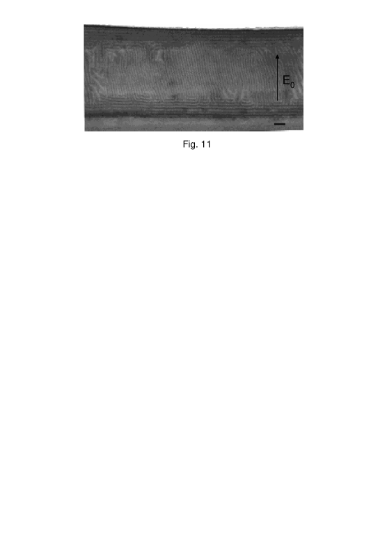
Figure 11: TEM cross section of thin-film PS/PMMA block copolymer annealed in electric field $E_{0}\simeq 40$ V/$\mu$m. Few lamellae lie parallel to the substrate (bottom) and polymer-air interface (top), while the rest of the film has lamellae parallel to the field. Adapted with permission from Xu et al. (2004b). Copyright 2002 American Chemical society.

Muthukumar has considered other confined ordered phases in electric field by using a similar model. While the dependence of the transition field between parallel and perpendicular orientations on $L$ is weak for lamellae, they find that for cylinders the $L$ dependence of the energy is more complicated, and the transition field changes markedly as the film thickness changes Ashok et al. (2001).

III.3.2 Electrostatics of weakly segregated structures

The above derivations are valid in materials (not necessarily block copolymers) where the dielectric interfaces are sharp and $\Delta\varepsilon$ is large compared to the average permittivity $\bar{\varepsilon}$. Close to the critical point, however, the composition differences between coexisting phases become small. The expressions for the electric field and electrostatic energy given below only assume small $\varepsilon({\bf r})$ variations and therefore are general and not restricted to BCPs. The smallness of $\varepsilon$ variations, as compared to $\bar{\varepsilon}$, enables us to exactly solve Laplace’s equation for an arbitrary spatial distribution $\varepsilon({\bf r})$. Close to the critical point, we may write the order parameter as a sum of Fourier harmonics [Eq. (III.1)], with $\varphi({\bf r})\ll 1$. Consequently, only linear terms are retained in the constitutive relation $\varepsilon(\phi)$ and in the expansion of ${\bf E}$ in powers of $\varphi$ [Eqs. (3) and (4)]. The deviation of the electric field from its average, ${\bf E}_{1}\varphi$ in Eq. (4), is found by writing Laplace’s equation $\nabla\cdot(\varepsilon{\bf E})=0$ to linear order in $\varphi$ and is given by Amundson et al. (1993),

$$\varphi{\bf E}_{1} = \sum_{\bf q}{\bf E_{q}}e^{i{\bf q}\cdot{\bf r}}~{},$$ (30)

$${\bf E}_{\bf q} = -\frac{\Delta\varepsilon\varphi_{\bf q}}{\bar{\varepsilon}}\left(\hat{\bf q}\cdot{\bf E}_{0}\right)\hat{\bf q}~{}.$$

The electrostatic energy per unit volume can be approximated by

$$f_{\rm es}=\frac{(\Delta\varepsilon)^{2}}{2\bar{\varepsilon}}\sum_{\bf q}(\hat{\bf q}\cdot{\bf E}_{0})^{2}\varphi_{\bf q}\varphi_{-{\bf q}}+{\rm const.}$$ (31)

The constant on the right-hand side is the electrostatic energy for a uniform phase with $\phi({\bf r})=\phi_{0}$. Any plane-wave composition deviation $\varphi_{\bf q}e^{i{\bf q}\cdot{\bf r}}$ from the isotropic background leads to an electrostatic penalty. This energy, quadratic in $E_{0}$ as usual, is also quadratic in $\varphi_{\bf q}$. This is because in uniform electric fields, composition fluctuations $\varphi$ give rise to dielectric deviations $\delta\varepsilon\propto\varphi$ and electric-field deviations $\delta E\propto\varphi$, so the leading order term in the free energy density $-(1/2)\varepsilon E^{2}$ scales as $\varphi^{2}$.

The torque ${\bf N}$ acting on a sample of volume $\cal{V}$ in external field ${\bf E}_{0}$ consistent with the energy formula [Eq. (31)] is Tsori et al. (2003b):

$${\bf N}_{\rm dielec} = -2\mathcal{V}\frac{(\Delta\varepsilon)^{2}}{\bar{\varepsilon}}{\bf\Gamma}(\phi,{\bf E}_{0})$$ (32)

$${\bf\Gamma}(\phi,{\bf E}_{0}) = \sum_{\bf q}\varphi_{\bf q}\varphi_{-{\bf q}}(\hat{\bf q}\cdot{\bf E}_{0})\hat{\bf q}\times{\bf E}_{0}~{}.$$

An important feature of Eqs. (31) and (32) is the dependence on the angle between ${\bf q}$ and ${\bf E}_{0}$. If ${\bf q}$ and ${\bf E}_{0}$ are perpendicular to each other (dielectric interfaces parallel to ${\bf E}_{0}$), the energy is minimal and the torque vanishes. When ${\bf q}$ and ${\bf E}_{0}$ are parallel (interfaces perpendicular to ${\bf E}_{0}$), the torque vanishes, but the energy is highest.

Equation (31) is a useful formula for the calculation of electrostatic effects in soft-matter systems close to a critical point. When it complements a proper Ginzburg-Landau expansion of the energy in powers of $\varphi$, it enables rather easy derivation of various thermodynamical expressions on the mean-field level Onuki (2002). This issue will be discussed in Sec. IV.

III.3.3 Numerical calculations

A numerical approach for the calculation of electrostatic effects in spatially nonuniform materials has the advantage that it does not assume that $\Delta\varepsilon/\bar{\varepsilon}$ is small or large. Numerical calculations therefore bridge the gap between weak- and strong-segregation theories outlined above. Electrostatic calculations for block copolymers have been so far implemented by mean-field self-consistent field theory (SCFT). In SCFT of block copolymers, the Hamiltonian contains chain stretching penalty and enthalpic interactions, originating from unfavorable contacts between chemically different monomers. The partition function is expressed in terms of the density operators of the different types of monomers. The so-called restricted chain partition function obeys a modified diffusion equation Matsen and Schick (1994). In order to account for electrostatic effects, a constitutive relation $\varepsilon(\phi)$ is chosen (usually a linear relation), and the electrostatic energy $F_{\rm es}$ in Eq. (1) is added to the Hamiltonian. The full set of equations must be solved self-consistently together with Laplace’s equation and subjected to the proper boundary conditions on the electrodes, i.e., Dirichlet, Neumann, or mixed boundary conditions Lin et al. (2005); Matsen (2006b). The main advantage of the formalism for this study is the exact calculation of electrostatic energy - the numerical procedure does not rely on the analytical approximations such as Eq. (31).

While static calculation pertains to equilibrium morphologies, a certain variant of SCFT allows description of the dynamical relaxation toward equilibrium. In the scheme developed Sevink et al. (1999), the free energy is calculated similarly to the static case. The time variation in the order parameter $\phi$ is then assumed to obey the following dynamics Onuki (2002):

$$\frac{\partial\phi}{\partial t}=M\nabla^{2}\mu+\eta~{},$$ (33)

where the chemical potential $\mu$ is a functional derivative of the total free energy including $F_{\rm es}$, $M$ is a proper Onsager mobility coefficient (usually taken to be constant), and $\eta$ is a noise term satisfying the fluctuation-dissipation theorem. This approach does not fully take into account the polymer viscoelastic flow and reptation effects. In addition, the Amundson-Helfand quadratic electrostatic energy approximation [Eq. (31)] was used instead of the full expression Schmidt et al. (2007). Still, a reasonable match with experiment was found: the simulations report an exponential relaxation of the order parameter $S(t)$ [Eq. (23)], consistent with experiments Böker et al. (2003).

It should be stressed that the approach utilized above, that $\varepsilon$ is a simple scalar quantity, may fail with some polymers. Recent experiments show a peculiar phenomena, whereby the lamellar period changes by as much as $5\%$ under the influence of an electric field parallel to the lamellae Schmidt et al. (2008). The researchers attribute the thinning of lamellae to an anisotropic response of the polymers (PS/PI). In essence, the single chain conformations of the PI block are affected by the field, and the coil becomes more prolate in a direction parallel to the field Gurovich (1994).

Lastly, the cylinders in Fig. 6(c) follow the curved electric field lines. The electric field introduces electrostatic (Maxwell) stress in the anisotropic sample, and this stress must be balanced by elastic forces. The competition between electrostatic and elastic forces has not received enough attention in the literature and should be further investigated.

III.4 Instability of block-copolymer interface in perpendicular electric field

In light of the normal-field instabilities described in Sec. II, one may ask whether a similar interfacial instability can also occur in block copolymers. The difference between self-assembled materials, such as block copolymers, and simple liquids is that besides their high viscosity they feature elastic behavior. Indeed lamellar phases, for example, have both bending and compression moduli. As a result, any deformation of the interface between the copolymers results in deviation from the optimum balance between interfacial and entropic energies. It turns out that an interfacial instability does occur in BCPs in electric field, and the nature of the instability depends on the distance from the critical point.

Onuki and Fukuda (1995) studied the strong-segregation regime by writing the copolymer composition as $\phi(x,z)=\phi_{0}+\varphi_{L}\cos[(2\pi/d)x+u(y)]$, with $\varphi_{L}$ as an amplitude and $d$ as the lamellar period, and expanding the energy in small $u$. They found an interfacial instability with two characteristics: (i) two adjacent A/B polymer interfaces are parallel to each other and (ii) the most unstable wavelength is long, corresponding to the lateral film size [Fig. 12(a)]. This instability is similar to the Helfrich-Hurault instability common in smectic and cholesteric liquid crystals de Gennes and Prost (1993).

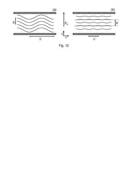
Figure 12: Schematic illustration of two normal-field instabilities in lamellar block copolymers (not to scale). $d$ is the unperturbed lamellar thickness and $\lambda^{*}$ is the undulation period. (a) In the strong-segregation regime, adjacent lamellae bend in phase with each other. $\lambda^{*}$ is macroscopic, $\lambda^{*}\gg d$. (b) Close to the ODT point, lamellae are easier to deform, and adjacent lamellae undulate out of phase with each other. $\lambda^{*}$ is equal to the lamellar thickness $d$.

A different scenario occurs close to the ODT (critical) point. In this regime, the composition variations are very weak, and lamellae are easy to deform. A stability analysis of the Ginzburg-Landau-like free energy expansion, appropriate close to a critical point and on the mean-field level, reveals that the most unstable wavelength $\lambda^{*}$ is the same as the bulk period $d$ [see Fig. 12(b)] Tsori and Andelman (2002). This is very different from the instability in the liquid case. Moreover, adjacent lamellae are out of phase with each other. At the onset of instability, the BCP morphology is essentially a superposition of two lamellar phases with normals parallel and perpendicular to the substrate. These modulations were also corroborated by a more accurate SCFT study Matsen (2005, 2006c), which describes undulatory “peristaltic” modes similar to that of Fig. 12. These theoretical predictions were essentially verified in experiment Xu et al. (2004a).

III.5 Role of residual ions

The preceding discussion of block copolymers assumes that the polymers are purely dielectric materials and ignores the possible existence of dissociated ions. However, almost all polymers have small conductivity due to the finite amount of ions in them. For example, in anionic polymerization the reaction typically starts with an organometallic reagent, such as butyl lithium. At the end of the reaction, each chain is neutralized with water, and one metal hydroxide ion (e.g., LiOH) is released. Thus, the average ion density is one ion per polymer chain, which is equivalent to a number density of $10^{25}$ m^-3 ($\simeq 0.016$M) or charge density of $1.6\times 10^{6}$ C m^-3.

Even without electric fields, a salt content adds to the molecular polarizability of the polymer, and therefore changes the interaction parameter $\chi$ between polymer molecules. In addition, like any chemical impurity, salt can change the interfacial interactions of the polymers with the substrate. The effect of ions on the BCP phase diagram was studied quantitatively Epps et al. (2002, 2003); Wang et al. (2008). For a given phase, we are interested in the effect ions have on the orientation process in external fields. Most of the salt content crystallizes and is found in neutral clusters inside the polymer, and only a small fraction ($10^{-3}-10^{-6}$) is dissociated and participates in the orientation mechanism. Of those ions, some are complexed to the polymer to which they have a preferential solubility, usually the more polar block. They increase the effective dielectric constant of the polymer and therefore increase the effective $\Delta\varepsilon$.

The rest of the ions are mobile; when subjected to electric field, they give rise to screening. Two extreme cases follow: in the first, the screening length $\lambda$ is much larger than the lamellar period $d$ and in fact may even be as large as the film thickness. When this happens, the ion cloud is uniformly distributed throughout the film in the more polar polymer, and the system behavior is similar to that of neat BCPs, only with effective $\varepsilon$’s. The critical field for transition from parallel to perpendicular lamellae still scales as $E\sim L^{-1/2}$. Orientation experiments were carried out on PS/PMMA samples doped with ions Xu et al. (2004a); Wang et al. (2006). Ions reside preferentially in the PMMA block, resulting in an increased $\Delta\varepsilon$ and correspondingly smaller fields for the orientation process. How much the dielectric constant of the PMMA block is enhanced depends on the frequency of applied field and on the temperature Kohn et al. (2009). Typically, the dielectric constant increases with decreasing frequency. Large doping with ions can lead to even a fivefold increase in the static dielectric constant.

The second extreme case corresponds to screening length $\lambda$ smaller than $d$ and occurs when salt is added. In this case, most of the ions concentrate at the electrodes. Here one expects the most polar polymer to wet the surface due to the preferential solubility of ions. The effect of electric field is thus reminiscent of electrowetting and can be approximately described by an effective interfacial energy between the polar block and the substrate. Note that in contrast to the case with neat BCPs, increase in the electric field increases the tendency of lamellae wetting parallel to the substrate. The effective surface tension depends on the total ion density and vanishes with vanishing electrode potential $V$. The mixed structure depicted in Fig. 9 is possible for intermediate screening lengths $\lambda\geq d$ and depends on the vicinity to the ODT point.

The physics of the problem is rich when the external field varies sinusoidally in time. When a time-varying electric field is applied, the positive charge will tend to migrate parallel to the field, while negative charge will move in the opposite direction in an oscillatory motion. There are four length scales in the problem: the BCP domain size is $d\sim 50$-$100$ nm, comparable to the polymer radius of gyration. The second is the electromagnetic wavelength, $2\pi c/(\omega\sqrt{\bar{\varepsilon}})$, where $\omega$ is the field’s frequency. The third length is the distance a single ion drifts in one half period of the electric field: $\pi e\bar{\mu}E_{0}/\omega$, where $\bar{\mu}$ is the average mobility. Lithium mobility in PMMA is estimated to be $\bar{\mu}\simeq(4$–$5)\times 10^{5}$ m²/J s. Typically the wavelength of light is much larger than both the drift length and the BCP period. Lastly, the system size $L$ is usually the largest length. There are three energy scales: one is the energy stored in the dielectric material per unit volume, $U_{\rm dielec}=\bar{\varepsilon}E_{0}^{2}$. The second energy is the thermal energy $k_{B}T$. The third energy is the amount of heat dissipated per unit volume due to Joule heating in one field cycle: $U_{\rm Joule}=2\pi E_{0}^{2}\sigma/\omega$. Using an average density of dissociated Li ions $n\sim 10^{21}$ m^-3, one obtains the average conductivity $\sigma=e^{2}n\bar{\mu}\sim 10^{-11}$ C/m V s. Thus, Joule heating begins to be important at low frequencies, $\omega<\omega_{c}$ [Eq. (21)], where here $\omega_{c}\sim 5$–$50$ s^-1.

The copolymers are anisotropic materials, and therefore the mobility of ions is spatially nonuniform. Ions will consequently drift in the direction which is “easy” for them, and this direction may not be collinear with the external field. As a result, a torque is applied on the sample. The total torque works to orient the sample in such a direction that it vanishes and the mechanical energy is at minimum. Clearly, the torque depends on the external field’s frequency: small $\omega$ and long period means ions have a long way to drift before the field changes sign, and hence the torque exerted on the polymer matrix is large. At large values of $\omega$, ions are practically immobile and contribute nothing to orientation. A detailed calculation shows that the torque exerted by moving ions is dominant over the “dielectric interfaces” if $\sigma/\omega\gg\bar{\varepsilon}$. An expressions for the torque in this regime exists, and it reads as Tsori et al. (2003b)

$${\bf N}_{\rm ions}=-\frac{8\sigma}{\pi\omega}\mathcal{V}\left(\frac{\Delta\mu}{\bar{\mu}}\right)^{2}{\bf\Gamma}(\phi,{\bf E}_{0})~{}.$$ (34)

This formula should be contrasted with Eq. (32). It is valid close to the critical point and under the assumptions that positive and negative charges have equal mobilities and using a linear dependence of mobility on composition: $\mu(\phi)=\bar{\mu}+\varphi\Delta\mu$. In this regime, occurring when $\omega<\omega_{c}$, the mobile ions become increasingly important and the concept of dielectric contrast should be replaced by mobility contrast. In this regime the sample is being heated; in most experimental systems, however, this energy dissipation does not present a problem since heat is quickly removed from the system.

The stresses introduced by moving ions and by dielectric interfaces (Maxwell stress) can lead to real symmetry-changing phase transitions and not just to orientation. This will be discussed in subsequent sections.

IV Critical Effects in Polymer and Liquid Mixtures in Uniform Electric Fields

Up to this point, we described several instabilities and orientation effects occurring when two immiscible liquids or ordered phases of block copolymers are subjected to an external electric field. One may ask even a more basic question: how does an electric field affect the relative thermodynamic stability of the possible system phases? We turn to investigate this question on the mean-field level as is the practice throughout this text.

IV.1 Landau theory and experiments

We consider a bistable system, able of having two different states at a certain range of the parameters. For concreteness one may think of a binary mixture of two liquids. The treatment of liquid-vapor coexistence of pure molecules is quite similar, the main difference being the finite gas compressibility which means that the Clausius-Mossotti relation connects between $\varepsilon$ and density Zimmerli et al. (1999b, a); Hegseth and Amara (2004). What is the effect of a uniform electric field on the phase diagram of liquid mixtures? This issue was treated first by Landau and Lifshitz (1957). For simplicity of exposition, we consider a symmetric liquid mixture. The free energy density in the absence of field, $f_{m}$, can be written as a Landau expansion valid close to the critical point,

$$\frac{v_{0}}{k_{B}T_{c}}f_{m}=\frac{1}{2}\frac{T-T_{c}}{T_{c}}\varphi^{2}+\frac{u}{4!}\varphi^{4}~{}.$$ (35)

Here $\varphi$ is the deviation of the composition from the critical composition ($1/2$), $v_{0}$ is a volume derived from the second virial coefficient, and $u$ is positive. We use the constitutive relation [Eq. (3)] to write the electrostatic energy density $f_{\rm es}\simeq-\frac{1}{2}\varepsilon_{c}E_{0}^{2}-\frac{1}{2}\Delta\varepsilon\varphi E_{0}^{2}-\frac{1}{4}\varepsilon^{\prime\prime}\varphi^{2}E_{0}^{2}$. The constant term is unimportant and the linear term can be eliminated by a redefinition of the chemical potential. The only important term is the quadratic one. Inspection of $f=f_{m}+f_{\rm es}$ shows that since $f_{\rm es}$ is small, close enough to $T_{c}$, that $f_{\rm es}$ simply serves to redefine the critical temperature. Thus

$$T_{c}\to T_{c}+\Delta T_{c}~{},$$

$$\Delta T_{c}=\frac{v_{0}\varepsilon^{\prime\prime}E_{0}^{2}}{2k_{B}}~{}.$$ (36)

$T_{c}$ and the whole binodal curve are increased if $\varepsilon^{\prime\prime}$ is positive, and in this case electric field leads to demixing. If $\varepsilon^{\prime\prime}<0$, then $T_{c}$ is decreased and mixing is favored. We use the value $v_{0}\sim 10^{-28}$ m³ and average electric field $E_{0}\sim 10$ V/$\mu$m to obtain the typical shift to $T_{c}$ due uniform fields in either case to be $v_{0}\varepsilon^{\prime\prime}E_{0}^{2}/k_{B}\sim 30$ mK. Subsequent theoretical work employed a renormalization-group Onuki (1995a) and other approaches Sengers et al. (1980) to study the vicinity of the critical point, but the main result remained: $T_{c}$ changes by few milikelvins under the influence of moderate-to-strong fields.

The theory should be compared with experiments which followed. The first experiment was by Debye and Kleboth (1965) on mixture of isooctane and nitrobenzene, whose dielectric contrast is $\Delta\varepsilon=32.3\varepsilon_{0}$. Under an electric field of $4.5$ V/$\mu$m, they found that $T_{c}$ is reduced by $15$ mK. These results were later verified with great accuracy by Orzechowski (1999). Debye’s experiments were followed by a work of Beaglehole (1981). He worked on a cyclohexane/aniline mixture with $\Delta\varepsilon=5.8$ and in a field of $0.3$ V/$\mu$m. $T_{c}$ was found to be reduced by as much as $80$ mK. Early (1992) worked on the same mixture with similar fields. He found that $T_{c}$ does not change at all and hinted that previous results were due to spurious heating occurring in dc fields. Wirtz and Fuller (1993) worked on n-hexane/nitroethane mixture with $\Delta\varepsilon=17.7\varepsilon_{0}$ and found a reduction in $T_{c}$ by $20$ mK.

The experiments above are in contradiction to theory since mixing is observed instead of demixing even though $\varepsilon^{\prime\prime}>0$. In addition, there were wrong signs in some experiments as well as theory. More importantly, in both theory and experiment the change to $T_{c}$ is much smaller than $100$ mK. The only exception is the work of Reich and Gordon (1979), who worked on a polymer-polymer mixture having a lower critical solution temperature (LCST) and found that $T_{c}$ changes by about $4$ K or even more under an electric field of $\sim 10$ V/$\mu$m. Two comments on the big effect observed are the following: (i) The large molecular volume of polymers means their entropy is reduced. $v_{0}$ should be replaced by $Nv_{0}$ in Eq. (36). (ii) Heating, if present in a LCST system in the homogeneous phase, may lead to demixing, as is observed in these experiments.

A possible explanation for the mixing observed in experiments is due to the dielectric anisotropy not accounted for by Eq. (36). Indeed, just as with block copolymers or any other anisotropic material, composition variations $\varphi$ lead to dielectric constant variations $\delta\varepsilon$. Compliance to Laplace’s equations means that the electric field has variations too, and in linear order $\delta E\propto-\delta\varepsilon$. As is clear from Eqs. (III.1) and (31), the electrostatic free energy contribution $f_{\rm es}$ scales quadratically with $\varphi$. We therefore conclude that the prefactor of $\varphi^{2}$ in a Landau series expansion of $f_{m}+f_{\rm es}$ around the critical composition has two terms: one proportional to $-\varepsilon^{\prime\prime}$ and the second to $+(\Delta\varepsilon)^{2}$. A positive $\varepsilon^{\prime\prime}$ favors demixing while $(\Delta\varepsilon)^{2}$ term promotes mixing and is usually dominant.

Light-induced phase transitions in mixtures

We briefly mention several cases where light influences the morphology of mixtures. Light in the UV range was applied on polymer blends of stilbene-labeled polystyrene and polyvinylmethylether (PSS/PVME). This caused phase separation of the blend because trans$\to$cis transition changes both the volume and the enthalpic interaction between the polymers Nishioka et al. (2000). In addition, photochemical reaction was induced in anthracene-labeled polystyrene-PVME blends irradiated by periodic UV light. The distribution of length scales in the resulting spinodal decomposition depends sensitively on the applied frequency Tran-Cong-Miyata et al. (2004).

Even in the absence of chemical activity, an intense laser beam can lead to a mixing or demixing phase transition. Poly($N$-isopropylacrylamide) (PNIPAM) – water and PNIPAM – D₂O mixtures were illuminated by tightly focused laser light in the infrared wavelength Ishikawa et al. (1996); Hofkens et al. (1997). These mixtures have LCST (inverted) phase diagrams and the initial temperature corresponded to a homogeneous state. Aggregation of the polymer was observed in the region illuminated by the laser. Two possible explanations were suggested. First, water adsorption in the infrared regime causes heating, and in a LCST system this may cause phase separation. Second, radiation pressure supposedly works in conjunction with the heating to separate the polymer from the solvent and to accumulate it in micron-scale aggregates. Subsequent work Borowicz et al. (1997) was similar, but now poly($N$-vinylcarbazole) was dissolved in two different organic solvents, cyclohexanone and $N$,$N$-dimethylformamide. This work showed that the segregation of polymer from the solvent occurs in the absence of heating and is due to the strong laser electric field. The underlying physical mechanisms responsible for the observations were theoretically examined by Delville et al. (1999). In Sec. V we give a possible mechanism which may be relevant to equilibrium situations.

IV.2 Block-copolymer phase transitions

In Sec. III, block copolymer orientation in electric fields was described as a result of a “dielectric interfaces”, stemming from a term proportional to $(\Delta\varepsilon)^{2}$ in the free energy. Equation (32) shows that a BCP sample experiences a force as long as there are dielectric interfaces perpendicular to the external field. Phases with uniaxial symmetry thus turn until their axis of symmetry is parallel to ${\bf E}_{0}$. When this orientation terminates, their total electrostatic energy is exactly equal to $-\frac{1}{2}\bar{\varepsilon}E_{0}^{2}\times\mathcal{V}$, where $\mathcal{V}$ is the total volume. But there are ordered phases, such as the bcc phase of spheres, where frustration always occurs. As $E_{0}$ is increased, the crystal deforms, and the spheres elongate along the external field. This is reminiscent of the liquid droplet elongation described in Sec. II.1, but in addition to the interfacial tension and electrostatic energies, in BCPs there is also elastic energy that needs to be taken into account. With increasing value of $E_{0}$, the crystal deforms, until, at a certain critical value of $E_{0}$, its energy is no longer the lowest among all phases, and a phase transition occurs Tsori et al. (2003a).

The phase diagram close to the critical point can be calculated by a Landau expansion of the energy in series of $\varphi_{\bf q}$, given in Fourier space by

$$\frac{v_{0}}{k_{B}T_{c}}F = \frac{1}{2}\sum_{\bf q}\left[\frac{T-T_{c}}{T_{c}}+\frac{v_{0}(\Delta\varepsilon)^{2}}{\bar{\varepsilon}k_{B}T_{c}}(\hat{\bf q}\cdot{\bf E}_{0})^{2}\right.$$ (37)

$$+ \left.C(q^{2}-q_{0}^{2})^{2}\right]\varphi_{\bf q}\varphi_{-{\bf q}}+O(\varphi_{\bf q}^{3})~{}.~{}~{}~{}$$

The last term in the square brackets is specific to modulated phases such as block copolymers, and is absent in simple liquids. It expresses the penalty of having $q$ modes with $q$ different than the preferred inverse periodicity, $q_{0}=2\pi/d$. The prefactor $C$ contains information on the polymer, such as the radius of gyration. The electric field (second term) introduces a penalty proportional to the cosine squared of the angle between field and $q$ vector. As is mentioned above, this field-dependent term is usually quite small: when we replace $\varepsilon^{\prime\prime}$ by $(\Delta\varepsilon)^{2}/\bar{\varepsilon}$ in the estimate after Eq. (36), we get the same millikelvin-sized effect of renormalization of $T_{c}$. For block copolymers, however, the molecular weight can be large and thus, replacing $v_{0}$ by $Nv_{0}$, one may get a larger change to $T_{c}$, similar to the experiments on polymer mixtures Reich and Gordon (1979).

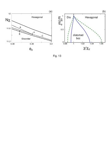
Figure 13: Block-copolymer phase diagrams. (a) Phase diagram for diblock copolymers in the ($\phi_{0}$,$\chi$) plane at fixed electric field. Two outer solid lines are zero-field hexagonal-to-bcc and bcc-to-disorder phase boundaries. Lines A and B are transitions from distorted bcc to the hexagonal and disordered phases, respectively, and line C is the boundary between hexagonal and disordered phases in electric field given by $(\varepsilon_{0}Nv_{0}/k_{B}T)^{1/2}E_{0}=0.2$. They meet at the triple point ($\phi_{0}$,$N\chi$)=($0.39$,$11.43$). Adapted from Lin et al. (2005). (b) Phase diagram in the ($E_{0}$,$\chi$) plane and fixed composition $\phi_{0}=0.3$. For low values of field, a distorted bcc phase lies between the disordered (“Dis”) and hexagonal phases. The phase lines terminate at a triple point ($\chi_{\rm tr}$, $E_{\rm tr}$). When $E_{0}>E_{\rm tr}$, the distorted bcc does not exist. Solid lines are from analytical one-mode approximation, whereas dashed lines are from self-consistent field theory. The axes of each calculation are scaled by the relevant values of $\chi_{\rm tr}$ and $E_{\rm tr}$. Adapted with permission from Lin et al. (2005) and Tsori et al. (2006). Copyright 2002 American Chemical society.

Figure 13(a) is a phase diagram in the ($\phi_{0}$,$\chi$) plane ($\chi\sim 1/T$) for fixed electric field, obtained with the SCFT approximation. A linear constitutive relation was used: $\varepsilon(\phi)=\bar{\varepsilon}+\Delta\varepsilon\varphi$. Solid lines are zero-field phase boundaries, while dotted lines marked with A, B, and C are the new phase boundaries in the presence of an external field. There appears a triple point where three phases meet. At values of $\phi_{0}$ smaller than the triple point value, a direct transition between hexagonal and disordered phases occurs as a function of $\chi$ (or $T$). Part (b) is a phase diagram in the ($\chi$, $E_{0}$) plane for fixed $\phi_{0}$. Dashed lines are a result of SCFT calculation, while the solid lines are from Eq. (37) augmented with higher order terms in $\Delta\varepsilon$ and $\varphi_{\bf q}$. The higher-order corrections in $\Delta\varepsilon$ are essential since an interchange of the dielectric constant of the A and B polymers does not leave the electrostatic energy invariant. As the electric field is increased from zero, the area occupied by the distorted bcc phase shrinks in favor of the disordered and hexagonal phases. The phase lines terminate at a triple point ($\chi_{\rm tr}$, $E_{\rm tr}$). The bcc phase completely disappears when $E>E_{\rm tr}$. The transition from spheres to cylinders was also studied for BCPs confined to thin films using SCFT. The deformation of the spheres from their perfect shape and the stability diagrams were calculated for the various system parameters Matsen (2006a).

In the above calculation, the zero-field critical point at $(N\chi$,$\phi_{0})\simeq(10.49,1/2)$ is left unchanged because of the linear relation $\varepsilon(\phi)$ and because lamellae and cylinders suffer no electrostatic penalty once oriented along the external field. This is not true, however, if the constitutive relation has a nonvanishing quadratic dependence. To see that this dependence can change the ODT point, consider $\varepsilon^{\prime\prime}\neq 0$ in Eq. (3), and $\varphi=\varphi_{L}\cos(qx)$ [see Eq. (III.1)], $\phi_{0}=1/2$ (symmetric lamellae), and ${\bf E}_{0}$ is in the $y$ or $z$ directions. We find that $f_{\rm es}=-(1/2)\bar{\varepsilon}E_{0}^{2}-(1/8)\varepsilon^{\prime\prime}\varphi_{L}^{2}E_{0}^{2}$. The electrostatic energy of the disordered phase is $f_{\rm es}=-(1/2)\bar{\varepsilon}E_{0}^{2}$, and therefore the electrostatic energy favors oriented lamellae over disorder if $\varepsilon^{\prime\prime}>0$; on the other hand, when $\varepsilon^{\prime\prime}<0$ lamellae are expected to melt for large enough field even if they are oriented in the “right” direction.

Lastly, we mention that the non-mean-field effect of uniform electric fields on composition fluctuations in symmetric block copolymers has been calculated as well. The weak first-order phase transition occurring in short polymers is shifted closer to the mean-field value, that is, the ODT point is shifted to higher temperatures Gunkel et al. (2007); Stepanow and Thurn-Albrecht (2009). As a result, phase separation is favored even if $\varepsilon^{\prime\prime}=0$. The shift to the ODT temperature was estimated to be about $2.5$ K. A systematic measurement of the constitutive relation $\varepsilon(\phi)$ is required in order to compare theory and experiment and to distinguish which of the terms – $\Delta\varepsilon$ leading to mixing, fluctuation effect leading to demixing, or $\varepsilon^{\prime\prime}$ leading to either mixing or demixing – is dominant in order-order phase transitions in polymer systems.

V Liquid Mixtures in Electric Field Gradients

Up to this point we have been primarily interested in uniform fields. Since even inside an ideal parallel-plate condenser composition inhomogeneities lead to nonuniform fields, we defined uniform fields as those present in the system if the dielectric constant is uniform. In the language of Eq. (4), this means ${\bf E}_{0}$ is constant. Spatially nonuniform fields have important consequences: they break the translational and the rotational symmetries, and therefore the symmetry of the phase diagram around $\phi_{c}$ is also broken. For a bilayer of two liquids in perpendicular electric field [Fig.  1(a)] a uniform field ${\bf E}_{0}$ deforms the interface only above a certain value, whereas a nonuniform field ${\bf E}_{0}$ deforms an interface no matter how small its strength is. Mathematically, when ${\bf E}_{0}$ is nonuniform the linear terms in $\varphi$ in the expansion of $f_{\rm es}$ [Eq. (5)] survive the integration. The resulting dielectrophoretic force tends to “suck” material with high $\varepsilon$ toward regions with high values of $E^{2}$.

As before, we stick for concreteness to a binary mixture of two simple liquids, denoted 1 and 2, with similar molecular volumes. The conclusions we draw are valid with only small modifications also to liquid-vapor coexistence in field gradients. The mixture free energy as a function of composition, $f_{m}(\phi)$, is taken to be symmetric with respect to $|\phi-1/2|$. The mixture has an upper consolute point; if $T>T_{c}$ the energy is convex at all compositions and the mixture is homogeneous. Below $T_{c}$, $f_{m}$ has a double-minimum shape. The transition (binodal) curve $\phi_{t}(T)$ is given by $df_{m}(\phi_{t},T)/d\phi=0$.

We start with neat dielectric liquids, and in Sec. V.2 we generalize to ion-containing liquids.

V.1 Ion-free mixtures

The mixture is subject to electric field emanating from a collection of conductors $1$, $2$, . . . , $N$, with prescribed potentials $\psi_{1}$, $\psi_{2}$, . . . , $\psi_{N}$, or charged with charges $Q_{1}$, $Q_{2}$, . . . , $Q_{N}$ each. We are interested in finding the potential distribution $\psi({\bf r})$ and composition profile $\phi({\bf r})$ as a function of the external potentials or charges. The total free energy density is given by

$$f=f_{m}(\phi)-\frac{1}{2}\varepsilon(\phi)\left(\nabla\psi\right)^{2}-\mu\phi~{}.$$ (38)

The equilibrium profiles are governed by the following Euler-Lagrange equations:

$$\frac{\delta f}{\delta\phi} = \frac{\delta f_{m}}{\delta\phi}-\frac{1}{2}\frac{d\varepsilon}{d\phi}\left(\nabla\psi\right)^{2}-\mu=0~{},$$ (39)

$$\frac{\delta f}{\delta\psi} = \nabla\left(\varepsilon(\phi)\nabla\psi\right)=0~{}.$$

In these equations, $\mu$ is the chemical potential needed to conserve the average mixture composition $\phi_{0}$,

$$\mathcal{V}^{-1}\int\phi({\bf r}){\rm d}^{3}r = \phi_{0}~{},$$ (40)

where ${\mathcal{V}}$ is the volume or is the reservoir chemical potential in case of a grand-canonical ensemble. The second variational equation is simply the Laplace equation. The set of differential equations [Eq. (39)], are coupled and nonlinear and quite difficult to solve. Above $T_{c}$, $f_{m}(\phi)$ is convex. We therefore expect that under the spatially nonuniform forcing of the external field the composition $\phi({\bf r})$ will be a smoothly varying function of space. Variations in $\phi$ will be proportional to the variations in field, and if $E_{0}({\bf r})$ is continuous, so is $\phi({\bf r})$.

Below $T_{c}$, this is not true, and one can expect a different behavior as is shown below. Consider three “canonical” examples illustrated in Fig. 14. The first one is a charged isolated spherical colloid of radius $R_{1}$ and total charge $Q$ coupled to a reservoir at infinity. Azimuthally symmetric profiles depend on $r$ only, where $r$ is the distance from the colloid’s center. Thus $\phi=\phi(r)$, $\varepsilon=\varepsilon(r)$, and the field is given by ${\bf E}(r)=Q/\left(4\pi\varepsilon[\phi(r)]r^{2}\right)\hat{\bf r}$. The second geometry is a charged wire of radius $R_{1}$ and charge $\lambda$ per unit length, coupled to a reservoir at $r\to\infty$. Alternatively, we may consider a closed condenser made up of two concentric cylinders with fixed average mixture composition. In both cases the electric field is ${\bf E}(r)=\lambda/\left(2\pi\varepsilon[\phi(r)]r\right)\hat{\bf r}$. A third system is the so-called “wedge,” made up from two flat electrodes with an opening angle $\beta$ between them, with potential difference $V$. In the wedge, ${\bf E}$ is given by ${\bf E}=V/(\beta r)\hat{{\bf\theta}}$, irrespective of the profiles $\phi(r)$ or $\varepsilon(r)$. The dielectrophoretic force existing in the wedge condenser may lead to discontinuous meniscus location in immiscible liquids Jones (1974), or to exact cancellation of gravity effects in mixtures near their critical point Tsori and Leibler (2005).

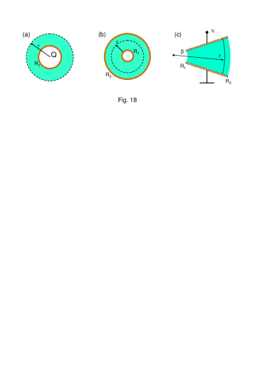
Figure 14: Three model systems where field gradients lead to demixing. (a) A single charged colloid of charge $Q$ and radius $R_{1}$. (b) A charged wire with charge density $\lambda$ per unit length and radius $R_{1}$ or two concentric cylinders with radii $R_{1}$ and $R_{2}$. (c) A wedge comprised of two flat electrodes with an opening angle $\beta$ and potential difference $V$. $R_{1}$ and $R_{2}$ are the minimal and maximal values of the distance $r$ from the imaginary meeting point.

Nonuniform electric fields will not demix liquids such that liquid interfaces are created parallel to the field. To see this, consider the two concentric cylinders with potential difference $V$. In the homogeneous state, $\varepsilon=\bar{\varepsilon}=\phi_{0}\varepsilon_{1}+(1-\phi_{0})\varepsilon_{2}$ is uniform. The demixed state has two uniform liquids of permittivities $\varepsilon_{1}$ and $\varepsilon_{2}$ occupying two portions of relative volumes $\phi_{0}$ and $1-\phi_{0}$, respectively, and the interfaces are parallel to ${\bf E}$. The homogeneous and demixed states have exactly the same electric field and same value of $F_{\rm es}$, but $F_{m}$ is higher for the demixed state. If the inner cylinder has a charge $\lambda$ per unit length immobilized to it, then the difference in $F_{\rm es}$ between the demixed and the homogeneous states is $\lambda^{2}/(4\pi)\ln(R_{2}/R_{1})[\phi_{0}/\varepsilon_{1}+(1-\phi_{0})/\varepsilon_{2}-1/\bar{\varepsilon}]$, and this difference is always positive.

The creation of interfaces perpendicular to the external field is in contrast to our intuition about uniform electric fields: despite the effects of dielectric interfaces, the dielectrophoretic force is the dominant mechanism. In addition, when a nonuniform field acts parallel to a liquid interface, it destabilizes it Jones (1972); Perry and Jones (1975).

Additional comment can be made on the possible mobility of charges inside the conductors: consider a single flat conductor at $x=0$, charged with average charge $\bar{\sigma}$ per unit area (uniform fields). The mixture is at the half space $x>0$ and has average dielectric constant $\bar{\varepsilon}$. Is it beneficial for the system to separate into two regions, one at $y>0$, with surface charge $\bar{\sigma}+\delta\sigma$ (at $x=0$) and dielectric constant $\bar{\varepsilon}+\delta\varepsilon$ (at $x>0$), and one at $y<0$, with surface charge $\bar{\sigma}-\delta\sigma$ ($y=0$) and dielectric constant $\bar{\varepsilon}-\delta\varepsilon$ ($x>0$)? Even without accounting for the reduced entropy of charges, this will not occur since the difference in $F_{\rm es}$ between demixed and homogeneous states is proportional to $(\delta\sigma/\bar{\sigma}-\delta\varepsilon/\bar{\varepsilon})^{2}$ and is always positive. Patches can be created on the conductor’s surface, though, if the charges have effective repulsion due to van der Waals forces Naydenov et al. (2007).

Let us return to demixing in nonuniform fields. The nice thing about the three examples in Fig. 14, besides the geometrical simplicity, is the decoupling between the two equations [Eqs. (39)]. Essentially, we have already solved for Laplace’s equation and only need to substitute the value of $E$ in the variation with respect to $\phi$. We are left with a single nonlinear equation for $\phi(r)$, which has spatial dependence. Let us ignore for the moment the term proportional to $(\nabla\phi)^{2}$ in $f_{m}$. This can be justified because we are dealing with a volume term in $E^{2}(r)$. For a large system, the surface tension term acts only at sharp interfaces and can be neglected as a first approximation. For smaller systems, surface tension smooths out the composition profile $\phi(r)$ and the neglect cannot be justified.

In order to be concrete, consider the wedge geometry coupled to a reservoir at composition $\phi_{0}$ ($R_{2}\to\infty$) and assume that $\varepsilon$ varies linearly with $\phi$ [$\varepsilon^{\prime\prime}=0$ in Eq.(3)]. We find the equation for $\varphi$ is

$$f_{m}^{\prime}(\varphi)=\frac{1}{2}\Delta\varepsilon\left(\frac{V}{\beta r}\right)^{2}+\mu$$ (41)

(recall that $\varphi=\phi-\phi_{c}$ is the deviation from critical composition). In the absence of field, the composition is $\phi_{0}$, corresponding to a homogeneous phase above the binodal. With electric field, Eq. (41) gives an algebraic relation between $\varphi$ and $r$. Above $T_{c}$, the left-hand side is a monotonously increasing function behaving qualitatively as $\varphi+\varphi^{3}$. Therefore, $\varphi$ increase monotonically as $r$ decreases. This is the regular dielectrophoretic effect.

However, below $T_{c}$, the left-hand side has a sigmoidal shape; it behaves qualitatively as $-\varphi+\varphi^{3}$. One may plot $f_{m}^{\prime}(\varphi)$ against $\varphi$ at a fixed temperature. The graphical solution to Eq. (41) is then given as an intersection between this curve and a horizontal line independent of $\varphi$. At large values of $r$ (small electric field), the intersection occurs at negative values of $\varphi$. As $r$ decreases, $\varphi(r)$ increases. If the maximum field in the system $V/(\beta R_{1})$ is small, then the profile is still monotonic. If, however, $V$ is large enough, the solution to $\varphi$ to Eq. (41) occurs at negative values for large $r$’s and positive values for small $r$’s (large field). Necessarily, there is a location $r$ where $\varphi$ has a “jump.” This is the field-induced phase transition: at a certain value of the voltage, the profile becomes discontinuous Tsori et al. (2004); Marcus and Tsori (2009). After demixing occurs, the wedge exhibits two regions with different compositions separated by a sharp interface. The two compositions of the coexisting phases are themselves nonuniform.

The interface separating high and low values of $\phi$ is at $r=R$ ($R_{1}<R<R_{2}$). The critical potential $V^{*}$ is the minimal potential for demixing, and it occurs when $R$ attains its smallest value, i.e., $R=R_{1}$. As the potential increases, the interface moves to larger radii, and, in addition, the composition difference between the coexisting domains increases. For a closed wedge with average composition $\phi_{0}$, one readily finds that $R(V)$ is bounded, and the maximum value of $R$ is given by $R_{\rm max}^{2}=(1-\phi_{0})R_{1}^{2}+\phi_{0}R_{2}^{2}$. If the wedge is coupled to an external reservoir and $R_{2}=\infty$, $R$ grows indefinitely as a function of $V$.

The dimensionless potential $M_{w}$ can be written as $M_{w}\equiv V^{2}Nv_{0}\varepsilon_{0}/4\beta k_{B}T_{c}R_{1}^{2}$. Here we generalize to mixtures of polymers, $N$ is the polymerization index and $Nv_{0}$ is the total chain volume. Close enough to the transition composition $\phi_{t}$, the critical value of $M_{w}$, $M_{w}^{*}$, is bounded by the following expression:

$$M_{w}^{*}=\frac{\phi_{t}-\phi_{0}}{4\Delta\tilde{\varepsilon}}\frac{T}{T_{c}}\frac{d^{2}\tilde{f}_{m}(\phi_{t})}{d\phi^{2}}g(R_{2}/R_{1})~{},$$ (42)

where we have used $\Delta\tilde{\varepsilon}=\Delta\varepsilon/\varepsilon_{0}$, and $\tilde{f}_{m}=Nv_{0}f_{m}/k_{B}T$. $g(x)=2(x^{2}-1)/(x^{2}-1-2\ln x)$ is a geometry-specific dimensionless function of the ratio $x\equiv R_{2}/R_{1}$. Figure 15(a) shows $M_{w}^{*}$ as a function of difference between the transition composition $\phi_{t}$ and $\phi_{0}$. Solid lines are Eq. (42), while symbols are taken from a more accurate numerical calculation. Clearly, $M_{w}$ increases almost linearly with $\phi_{t}-\phi_{0}$. The slope decreases at $T$ approaches $T_{c}$. Note that the similarity between the wedge capacitor and a rapidly rotating centrifuge allows us to predict phase-separation transitions for mixtures in centrifuges if the rotation frequency is higher than a certain critical frequency Tsori and Leibler (2007b).

The behavior in the cylindrical (2D) and spherical (3D) cases is similar to the one described above for the wedge. There are expressions for the critical values of the dimensionless charges for the cylindrical and spherical symmetries: $M_{c}\equiv\lambda^{2}Nv_{0}/16\pi k_{B}T_{c}R_{1}^{2}\varepsilon_{0}$ and $M_{s}\equiv Q^{2}Nv_{0}/64\pi k_{B}T_{c}R_{1}^{4}\varepsilon_{0}$, respectively. Figure 15(b) shows the critical values for demixing, $M_{c}^{*}$ and $M_{s}^{*}$, as a function of temperature for three different compositions. Open symbols are calculated values of $M_{c}^{*}$ for two concentric cylinders, whereas filled symbols are $M_{s}^{*}$ for an isolated spherical colloid. For a given composition, curves only start above the transition temperature ($T/T_{c}\simeq 0.865$, $0.944$, and $0.986$ for $\phi_{0}=0.2$, $0.3$, and $0.4$, respectively). Note that in general, $M_{s}^{*}$ and $M_{c}^{*}$ are much larger than $M_{w}^{*}$ – this is again because of the dielectric interfaces: in the spherical and cylindrical symmetries, ${\bf E}$ is parallel to $\nabla\phi$, and therefore the dielectrophoretic force $\propto\Delta\varepsilon$ has to be large enough in order to overcome the penalty associated with dielectric interfaces, $\propto(\Delta\varepsilon)^{2}$. In the wedge ${\bf E}\perp\nabla\phi$, and $M_{w}^{*}$ is correspondingly smaller.

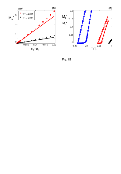
Figure 15: Critical demixing fields. (a) Scaled critical voltage for demixing $M_{w}^{*}$ for a closed wedge as a function of distance from the transition (binodal) composition $\phi_{t}$. Symbols are numerical values and line is approximate analytical expression [Eq. (42)]. (b) Scaled critical charge of spherical and cylindrical colloids as a function of temperature. Open symbols are $M_{c}^{*}$ for a closed cylindrical system of compositions $\phi_{0}=0.2$ (squares), $\phi_{0}=0.3$ (circles), and $\phi_{0}=0.4$ (crosses). Filled symbols are $M_{s}^{*}$ for an isolated spherical colloid coupled to a reservoir with the same compositions. Reprinted with permission from Marcus et al. (2008). Copyright 2008, American Institute of Physics.

How much should a $1$ $\mu$m colloid be charged to create a demixing layer around it? We take the molecular volume $v_{0}$ to be $3\times 10^{-27}$ m³, $N=1$ (simple liquids), and $T_{c}=350$ K. We find that $M_{s}^{*}=0.001$ leads to $Q\sim 10^{4}e$. This may seem like a large number; however, if the mixture contains even a low molecular weight polymer, then $N=500$ gives $Q\sim 470e$. The enrichment layer created around the colloid may be quite important for the thermodynamic behavior of suspensions because field-induced demixing leads to capillary attraction, promoting colloidal aggregation.

Finally, for a given value of $\phi_{0}$, there is an approximate expression for the range of temperatures $\Delta T$ above the transition temperature $T_{t}(\phi_{0})$ for which a given voltage is able to demix,

$$\Delta T=\frac{Nv_{0}}{2k_{B}}\left|\frac{\Delta\varepsilon}{\phi_{c}-\phi_{0}}\right|\left(\frac{V}{\beta R_{1}}\right)^{2}~{}.$$ (43)

This formula, applicable to the wedge, is valid close enough to the binodal. It should be contrasted with the Landau expression [Eq. (36)]. When the factor $N/2$ is put aside the two formulas have similar form: $\varepsilon^{\prime\prime}E_{0}^{2}$ in Eq. (36) is replaced by $\Delta\varepsilon(V/\beta R_{1})^{2}$, and both expressions have similar magnitudes since $\Delta\varepsilon/\varepsilon^{\prime\prime}\sim 1$. However, the denominator of Eq. (43) has the difference between $\phi_{0}$ and the critical composition. This factor means that $\Delta T$ here is at least twice as large as in the Landau case and typically is much larger: $|\phi_{c}-\phi_{0}|^{-1}\sim 20$ or even more.

The phenomenon described here has many similarities to regular prewetting. Important differences are (i) ${\bf E}$ is determined from Laplace’s equation and a similar equation does not exist for the case of long-range van der Waals forces between liquids and solid surfaces. (ii) In addition, the electric field needs not attain its highest value at the surface. Thus, “electroprewetting” is a special case of field-induced demixing. Consider an analogous system of a body of nonuniform heat conductivity $\kappa({\bf r})$ enclosed by a surface $\Sigma$ with prescribed temperature $T_{\Sigma}$. Temperature is the analog of $\psi$ and $\kappa$ is the analogue of $\varepsilon$. A question follows: is it possible to have a distribution $\kappa({\bf r})$ such that the steady-state temperature profile $T({\bf r})$ achieves a maximum or a minimum at the bulk rather than at $\Sigma$? A positive answer would mean that a confined mixture could spontaneously demix due to heat flow even without Soret or other effects. The answer to the question is negative. Since $T$ is governed by $\nabla(\kappa\nabla T)=0$, we find $\nabla\kappa\cdot\nabla T+\kappa\nabla^{2}T=0$, and extrema do not satisfy this equation because $\nabla T=0$ and $\nabla^{2}T\neq 0$. However, the point here is that electric fields are different: the fact that $\psi$ is largest on the electrodes does not prevent $E^{2}$ from being the largest elsewhere.

Up to this point, the liquids were considered as pure dielectrics. In the following section the phase-separation phenomenon is described in the presence of ions.

V.2 Phase separation in ion-containing liquids

The field-induced phase transition described above originates from electric-field gradients. In nonpolar liquids, such gradients occur when the electrodes are curved. In one dimension, e.g., in parallel-plate condenser, field gradients are forbidden by the equation $\nabla\cdot{\bf E}=0$. For curved electrodes, the geometry dictates the length scale over which the electric field falls off. On the other hand, mixtures of polar liquids (e.g., aqueous solutions) contain some amount of charge carriers. In such mixtures, the physics is rich and quite different from the simple dielectric case. The most important feature is due to screening, brought about by dissociated ions accumulating at the electrodes. Screening means that the electric field is substantial only close to the electrodes, within the screening distance $\lambda$. Field gradients originate from both geometry and screening, and the phase transition depends on two lengths. The ionic screening thus adds to the dielectrophoretic force which separates the liquid components from each other. Since screening is omnipresent, phase separation may occur even near parallel and flat charged surfaces, i.e., in one dimension.

But ions have another effect besides increasing the dielectrophoretic force. Ions have in general different solubilities in the different liquids. As an ion drifts toward the electrode, it might “drag” with it the preferred liquid component Onuki and Kitamura (2004). Usually the two ionic species are preferential in the same liquid, but it is also possible that they are preferentially soluble in different liquids. The solubility introduces a force of electrophoretic origin, proportional to the ions’ charge. In binary mixtures, the parameter $\Delta u^{+}$ measures how much a positive ion prefers to be in the environment of liquid 2 over that of liquid 1. To lowest order, the interaction per unit volume of positive ions and the mixture is given by $-\Delta u^{+}n^{+}({\bf r})\phi({\bf r})$, where $n^{+}$ is the positive ion number density. A similar expression exists for the negative ions. The system free energy density including the interaction of ions and field is given on the mean-field level by Onuki (2006); Onuki and Okamoto (2009)

$$f = f_{m}(\phi)-\frac{1}{2}\varepsilon(\phi)\left(\nabla\psi\right)^{2}+\left(n^{+}-n^{-}\right)e\psi$$

$$+ k_{B}T\left[n^{+}\ln\left(v_{0}n^{+}\right)+n^{-}\ln\left(v_{0}n^{-}\right)\right]-\lambda^{+}n^{+}$$

$$- \lambda^{-}n^{-}-\mu\phi-\left(\Delta u^{+}n^{+}+\Delta u^{-}n^{-}\right)\phi+{\rm const.}$$

In the above, $\lambda^{\pm}$ and $\mu$ are the Lagrange multipliers (chemical potentials) of the positive and negative ions and liquid concentration, respectively.

The free energy needs to be extremized with respect to the fields $\phi$, $\psi$, and $n^{\pm}$ in keeping with a fixed ion concentration ${\mathcal{V}}^{-1}\int n^{\pm}({\bf r}){\rm d}^{3}r=n_{0}$. The Poisson-Boltzmann equation is obtained from the variation in $f$ with respect to the potential and is coupled to $\delta f/\delta\phi$. This formalism is similar to other formulations, but the crucial difference is the bistability of the mixture energy $f_{m}$ Onuki and Kitamura (2004); Ben-Yaakov et al. (2009).

Solution to the problem is difficult to obtain because of the essential nonlinearity: a linear Poisson-Boltzmann equation does not suffice since imposing $e\psi\ll k_{B}T$ means small potential and thus forbids the large electric fields necessary to drive the phase-separation transition. The transition temperature $T_{t}(\phi_{0})$, defined by $df_{m}(\phi_{0},T_{t})/d\phi=0$, is shifted by an amount $\Delta T$ due to the external potential. An approximate formula for $\Delta T$ near a single planar electrode at $x=0$ can be obtained by the assumption that field gradients are dominated by ionic screening rather than by $\varepsilon$ variations. It reads Tsori and Leibler (2007a)

$$\frac{\Delta T}{T_{c}}\simeq\left(\frac{|\Delta\varepsilon|}{\varepsilon_{c}}+\frac{\Delta u}{k_{B}T_{c}}\right)\frac{Nn_{0}v_{0}}{|\phi_{c}-\phi_{0}|}\exp\left(\frac{eV}{k_{B}T_{c}}\right)~{},$$ (45)

where $\Delta u=\Delta u^{+}=-\Delta u^{-}$ and $V$ is the electrode potential. This expression holds as long as $T_{t}+\Delta T$ is smaller than $T_{c}$; at all temperatures $T>T_{c}$, the composition profile $\phi(x)$ varies smoothly with no abrupt jump. The shift in $T_{t}$ should be compared to Eq. (43) for a mixture without ions and to Eq. (36) for a mixture in uniform field. The dielectrophoretic and electrophoretic driving forces appear to have similar significance since both $\Delta\varepsilon/\varepsilon_{c}$ and $\Delta u/k_{B}T$ are $\sim O(1)$. The numerator has a small factor $Nn_{0}v_{0}$; in pure water and if we take $Nv_{0}=3\times 10^{-27}$ m³, we get $Nn_{0}v_{0}\sim 10^{-7}$. Small as this factor is, and even ignoring the denominator of $|\phi_{c}-\phi_{0}|$, the exponential factor $\exp(eV/k_{B}T)$ is the dominant term in $\Delta T$. It is usually huge, recalling that at room temperature $1$ eV equals $40k_{B}T$.

One can therefore expect that in almost all circumstances the electroprewetting discussed above should occur around a charged colloid in aqueous solutions. The width of wetting layer is small but may nonetheless influence the effective interaction potential between two colloids or between a colloid and a nearby surface Bauer et al. (2000) and the thermodynamic behavior of suspensions of charged particles Beysens and Estéve (1985). Electric field gradients may also play a role in such phenomena as the “critical Casimir effect,” recently reported experimentally by Hertlein et al. (2008).

The above wetting transition from a homogeneous to a demixed solution has several aspects. First, if the two or more constituent pure components have sufficiently differing indices of refraction, the optical properties of the solution will be drastically different in the two states. The demixing of an initially transparent solution leads to the creation of optical interfaces, and these can be used to scatter, reflect, and refract light. Particularly in a microfluidic environment, the phase separation could be utilized to create waveguides which are liquid and switchable Psaltis et al. (2006). The mechanical properties of the mixture are also different whether it is homogeneous or not. If the two pure components have different viscosities, as is the case of the experiments Tsori et al. (2004), then after demixing a thin lubricating layer is created at the charged surfaces, and this thin layer completely alters the flow profile between the surfaces. Finally, the field-induced phase separation can be used to control chemical reactions of, say, two molecules A and B reacting in a mixture of liquids 1 and 2. The dependence of concentration on electric field can accelerate the reaction or conversely stop it. The spatial dependence can be used to confine the reaction to small volumes or to two-dimensional interfaces Tsori and Leibler (2007a).

V.3 Phase separation in surfactant mixtures

Phase transitions in nonuniform electric fields are not restricted to demixing in liquid mixtures or to a liquid-vapor coexistence. In a set of beautiful experiments, Lee et al. (1994) demonstrated that a flat monolayer of a binary lipid mixture on the water-air interface undergoes a transition from a homogeneous to a phase-separated state when an insulated wire passing perpendicular to the monolayer is charged. The spatially varying electric field couples to the different dipole moments of the constituent molecules and attracts the molecules with large dipole toward the wire.

These experiments have an important difference from the demixing described before: the electric field couples to the fixed dipole of the lipids. Thus, the effect scales linearly with $E$ rather than quadratically. Consequently, when the wire potential is $V$, lipid 1 is attracted to the wire, whereas the potential reversal $V\to-V$ reverses the effect and accumulation of lipid 2 is observed at the wire. Note that the dipole orientation is restricted to be in one direction; if dipoles could flip upside down, a reversal of the field $E\to-E$ would leave the system invariant and the effect would again scale as $E^{2}$. Similarly to the demixing in simple liquids, below the critical pressure (which replaces $T$ in the phase diagram) only smooth gradients in $\phi$ appear, whereas below the critical pressure true demixing occurs, as evidenced by the sharp interface separating coexisting domains.

VI Conclusions

In this Colloquium we considered liquids and polymers in external electric fields. The key quantities for the physical behavior are the linear and quadratic coefficients in the expansion of $\varepsilon(\phi)$, namely, $\Delta\varepsilon$, and $\varepsilon^{\prime\prime}$ in Eq. (3), and the conductivity $\sigma$. We discussed the significance of these quantities in several phenomena occurring when the field is either spatially uniform or nonuniform. We have emphasized that in a uniform field ${\bf E}_{0}$, there is a preference of electrostatic origin to have dielectric interfaces parallel to ${\bf E}_{0}$. This preference, depending on $\Delta\varepsilon$, gives rise to the perpendicular field instability observed for liquid films discussed in Sec. II. The wavelength of instability $\lambda^{*}$ is the fastest-growing mode of a dynamical evolution. What is the smallest feature size possible in these experiments? The answer is not clear, and an effort is undertaken by several groups to minimize $\lambda^{*}$ by optimizing the fluid’s surface tension, film thickness, and other parameters. Dielectric interfaces are also responsible for block-copolymer orientation and order-order phase transitions in electric fields. Current effort focuses on finding ways to eliminate in-plane defects and enlarging the grain size. Destabilization of copolymer interfaces and polymer brushes may also occur, but here the wavelength is dictated by equilibrium considerations. In addition, a uniform electric field deforms the shape of suspended drops and of drops on solid substrates.

We have outlined some of the effects related to dissociated ions, commonly present in most simple and polymeric liquids. Finite conductivity introduces additional stress and can lead to oblate shapes of an isolated drop. Electrowetting is a result of charge accumulation at the droplet-substrate interface. The reduction in the droplet-substrate interfacial tension leads to an apparent change in the contact angle, and this has been widely used in applications. Ions also play an important role in copolymer orientation and phase transitions. Complexed ions mainly contribute to enhancement of $\Delta\varepsilon$, whereas mobile ones may give rise to wettinglike effects due to their preferential solubilities. An experimental effort is underway, aiming to understand when complexed ions are more dominant than mobile ones and vice versa. The study of electric-field-induced wetting of complex phases, such as block copolymers, is still at early stages and deserves experimental and theoretical treatments. Ions introduce stresses when the fields are time varying, and the resulting torques tend to orient the copolymer domains. The dynamics of these out-of-equilibrium systems is an open problem that also requires further investigation.

Uniform electric fields can also lead to phase transitions in liquid mixtures by the Landau mechanism. These transitions are insensitive to $\Delta\varepsilon$ but rely on nonvanishing $\varepsilon^{\prime\prime}$. Depending on the sign of $\varepsilon^{\prime\prime}$, the whole binodal curve can be shifted to higher or lower temperatures, but this shift is rather small, $\sim 0.03$ K.

Spatially nonuniform fields deform ordered block-copolymer phases due to a nonvanishing $\Delta\varepsilon$. The copolymer structure, a compromise between elastic bending and compression energies and the electrostatic energy, has not received enough attention so far. It is hoped that research in this direction can show us how to eliminate defects and perhaps even how to tailor lamellae or other phases in a prescribed way on a substrate. In the much simpler systems of liquid mixtures, bending is irrelevant, and nonuniform fields have a strong effect on the phase behavior. The direct coupling between field and composition leads to a phase transition which depends on $\Delta\varepsilon$ and cannot be simply described by a renormalization of $T_{c}$. The change in transition temperature is much larger than in the Landau mechanism. Wetting layers are created around curved charged objects but can also appear far from a solid interface. The presence of dissociated ions greatly enhances the transition and allows it to happen at flat objects. This transition can have numerous applications in microfluidics, in micro and nanorheology and lubrication, in chemical reactions, etc. The current study is only at its infancy and there is still plenty to learn: for example, what is the size and velocity of liquid domains appearing upon switching the field on, why interfacial instabilities are observed after demixing takes place, what is the role of critical fluctuations and the non-mean-field behavior, how does heating affects the transition, etc.

The phenomena outlined above are fundamentally interesting and also have numerous applications. We are certainly going to learn more about this active field of research in the years to come.

References

- Allan and Mason (1962) Allan, R. S., and S. G. Mason, 1962, Proc. R. Soc. London, Ser. A 267, 45.
- Amundson et al. (1991) Amundson, K., E. Helfand, D. D. Davis, X. Quan, S. S. Patel, and S. D. Smith, 1991, Macromolecules 24, 6546.
- Amundson et al. (1994) Amundson, K., E. Helfand, X. Quan, S. D. Hudson, and S. D. Smith, 1994, Macromolecules 27, 6559.
- Amundson et al. (1993) Amundson, K., E. Helfand, X. Quan, and S. D. Smith, 1993, Macromolecules 26, 2698.
- Andelman et al. (1986) Andelman, D., F. Brochard, P. G. de Gennes, and J. F. Joanny, 1986, C. R. Acad. Sci. 301, 675.
- Andelman et al. (1987) Andelman, D., F. Brochard, and J.-F. Joanny, 1987, J. Chem. Phys. 86, 3673.
- Andelman and Rosensweig (2009) Andelman, D., and R. E. Rosensweig, 2009, The Phenomenology of Modulated Phases: from Magnetic Solids and Fluids to Organic Films and Polymers (World Scientific, Singapore).
- Ashok et al. (2001) Ashok, B., M. Muthukumar, and T. P. Russell, 2001, J. Chem. Phys. 115, 1559.
- Bates and Fredrickson (1999) Bates, F. S., and G. H. Fredrickson, 1999, Physics Today 52((2)), 32.
- Bauer et al. (2000) Bauer, C., T. Bieker, and S. Dietrich, 2000, Phys. Rev. E 62, 5324.
- Beaglehole (1981) Beaglehole, D., 1981, J. Chem. Phys. 74, 5251.
- Ben-Yaakov et al. (2009) Ben-Yaakov, D., D. Andelman, D. Harries, and R. Podgornik, 2009, J. Phys. Chem. B 113, 6001.
- Berge (1993) Berge, B., 1993, C. R. Acad. Sci., Ser. II: Mec., Phys., Chim., Sci. Terre Univers 317, 157.
- Beysens and Estéve (1985) Beysens, D., and D. Estéve, 1985, Phys. Rev. Lett. 54, 2123.
- Bienia et al. (2006) Bienia, M., M. Vallade, C. Quilliet, and F. Mugele, 2006, Europhys. Lett. 74, 103.
- Böker et al. (2003) Böker, A., H. Elbs, H. Hänsel, A. Knoll, S. Ludwigs, H. Zettl, A. V. Zvelindovsky, G. J. A. Sevink, V. Urban, V. Abetz, A. H. E. Müller, and G. Krausch, 2003, Macromolecules 36, 8078.
- Böker et al. (2002) Böker, A., A. Knoll, H. Elbs, V. Abetz, A. H. E. Müller, and G. Krausch, 2002, Macromolecules 35, 1319.
- Borowicz et al. (1997) Borowicz, P., J.-I. Hotta, K. Sasaki, and H. Masuhara, 1997, J. Phys. Chem. B 101, 5900.
- Buehrle et al. (2003) Buehrle, J., S. Herminghaus, and F. Mugele, 2003, Phys. Rev. Lett. 91, 086101.
- Chou and Zhuang (1999) Chou, S. Y., and L. Zhuang, 1999, J. Vac. Sci. Technol. B 17, 3197.
- Cowley and Rosensweig (1967) Cowley, M. D., and R. E. Rosensweig, 1967, J. Fluid Mech. 30, 671.
- de Gennes and Prost (1993) de Gennes, P.-G., and J. Prost, 1993, The Physics of Liquid Crystals (Oxford University, New York).
- Debye and Kleboth (1965) Debye, P., and K. Kleboth, 1965, J. Chem. Phys. 42, 3155.
- Delville et al. (1999) Delville, J. P., C. Lalaude, and A. Ducasse, 1999, Physica A 262, 40.
- Du and Srolovitz (2004) Du, D., and D. Srolovitz, 2004, Appl. Phys. Lett. 85, 4917.
- Early (1992) Early, M. D., 1992, J. Chem. Phys. 96, 641.
- Epps et al. (2002) Epps, T. H. I., T. S. Bailey, H. D. Pham, and F. S. Bates, 2002, Chem. Mater. 14, 1706.
- Epps et al. (2003) Epps, T. H. I., T. S. Bailey, R. Waletzko, and F. S. Bates, 2003, Macromolecules 36, 2873.
- Etz et al. (1984) Etz, H., W. Gombert, W. Idstein, and P. Leiderer, 1984, Phys. Rev. Lett. 53, 2567.
- Garel and Doniach (1982) Garel, T., and S. Doniach, 1982, Phys. Rev. B 26, 325.
- Gunkel et al. (2007) Gunkel, I., S. Stepanow, T. Thurn-Albrecht, and S. Trimper, 2007, Macromolecules 40, 2186.
- Gurovich (1994) Gurovich, E., 1994, Macromolecules 27, 7339.
- Gurovich (1995) Gurovich, E., 1995, Phys. Rev. Lett. 74, 482.
- Hegseth and Amara (2004) Hegseth, J., and K. Amara, 2004, Phys. Rev. Lett. 93, 057402.
- Herminghaus (1999) Herminghaus, S., 1999, Phys. Rev. Lett. 83, 2359.
- Hertlein et al. (2008) Hertlein, C., L. Helden, A. Gambassi, S. Dietrich, and C. Bechinger, 2008, Nature (London) 451, 172.
- Hofkens et al. (1997) Hofkens, J., J. hotta, K. Sasaki, H. Masuhara, and K. Iwai, 1997, Langmuir 13, 414.
- Ishikawa et al. (1996) Ishikawa, M., H. Misawa, N. Kitamura, R. Fujisawa, and H. Masuhara, 1996, Bull. Chem. Soc. Jpn. 69, 59.
- Jones (1972) Jones, T. B., 1972, J. Appl. Phys. 43, 4400.
- Jones (1974) Jones, T. B., 1974, J. Appl. Phys. 45, 1487.
- Kohn et al. (2009) Kohn, P., K. Schröter, and T. Thurn-Albrecht, 2009, Phys. Rev. Lett. 102, 216101.
- Landau and Lifshitz (1957) Landau, L. D., and E. M. Lifshitz, 1957, Elektrodinamika Sploshnykh Sred (Nauka, Moscow), chap. II, Sec. 18, problem 1.
- Landau et al. (1984) Landau, L. D., E. M. Lifshitz, and L. P. Pitaevskii, 1984, Electrodynamics of Continuous Media (Butterworth-Heinemann, London), 2nd edition.
- Lee et al. (1994) Lee, K. Y. C., J. F. Klingler, and H. M. McConnell, 1994, Science 263, 655.
- Lin et al. (2005) Lin, C.-Y., M. Schick, and D. Andelman, 2005, Macromolecules 38, 5766.
- Lin et al. (2001) Lin, Z., T. Kerle, S. M. Baker, D. A. Hoagland, E. Schäffer, U. Steiner, and T. P. Russell, 2001, J. Chem. Phys. 114, 2377.
- Lin et al. (2002) Lin, Z., T. Kerle, T. P. Russell, E. Schäffer, and U. Steiner, 2002, Macromolecules 35, 3971.
- Lippmann (1875) Lippmann, G., 1875, Ann. Chim. Phys. 5, 494.
- Mansky et al. (1998) Mansky, P., J. DeRouchey, T. P. Russell, J. Mays, M. Pitsikalis, T. Morkved, and H. Jaeger, 1998, Macromolecules 31, 4399.
- Marcus et al. (2008) Marcus, G., S. Samin, and Y. Tsori, 2008, J. Chem. Phys. 129, 061101.
- Marcus and Tsori (2009) Marcus, G., and Y. Tsori, 2009, J. Phys. Soc. Jap. 78, 041010.
- Matsen (2005) Matsen, M. W., 2005, Phys. Rev. Lett. 95, 258302.
- Matsen (2006a) Matsen, M. W., 2006a, J. Chem. Phys. 124, 074906.
- Matsen (2006b) Matsen, M. W., 2006b, Macromolecules 39, 5512.
- Matsen (2006c) Matsen, M. W., 2006c, Soft Matter 2, 1048.
- Matsen and Schick (1994) Matsen, M. W., and M. Schick, 1994, Phys. Rev. Lett. 72, 2660.
- McConnell et al. (1984) McConnell, H. M., L. K. Tamm, and R. M. Weis, 1984, Proc. Natl. Acad. Sci. U.S.A. 81, 3249.
- Melcher and Schwartz (1968) Melcher, J. R., and W. J. Schwartz, 1968, Phys. Fluids 11, 2604.
- Melcher and Smith (1969) Melcher, J. R., and C. V. Smith, 1969, Phys. Fluids 12, 778.
- Morariu et al. (2003) Morariu, M. D., N. E. Voicu, E. Schäffer, Z. Lin, T. P. Russell, and U. Steiner, 2003, Nature Mater. 2, 48.
- Morkved et al. (1996) Morkved, T. L., M. Lu, A. M. Urbas, E. E. Ehrichs, H. M. Jaeger, P. Mansky, and T. P. Russell, 1996, Science 273, 931.
- Mugele and Baret (2005) Mugele, F., and J.-C. Baret, 2005, J. Phys.: Condens. Matter 17, R705.
- Mugele and Buehrle (2007) Mugele, F., and J. Buehrle, 2007, J. Phys.: Condens. Matter 19, 375112.
- Mugele and Herminghaus (2002) Mugele, F., and S. Herminghaus, 2002, Appl. Phys. Lett. 81, 2303.
- Naydenov et al. (2007) Naydenov, A., P. A. Pincus, and S. A. Safran, 2007, Langmuir 23, 12016.
- Nishioka et al. (2000) Nishioka, H., K. Kida, O. Yano, and Q. Tran-Cong, 2000, Macromolecules 33, 4301.
- O’Konski and Thacher (1953) O’Konski, C. T., and H. C. Thacher, 1953, J. Phys. Chem. 57, 955.
- Onuki (1995a) Onuki, A., 1995a, Europhys. Lett. 29, 611.
- Onuki (1995b) Onuki, A., 1995b, Physica A 217, 38.
- Onuki (2002) Onuki, A., 2002, Phase Transition Dynamics (Cambridge University Press, Cambridge).
- Onuki (2006) Onuki, A., 2006, Phys. Rev. E 73, 021506.
- Onuki and Fukuda (1995) Onuki, A., and J. Fukuda, 1995, Macromolecules 28, 8788.
- Onuki and Kitamura (2004) Onuki, A., and H. Kitamura, 2004, J. Chem. Phys. 121, 3143.
- Onuki and Okamoto (2009) Onuki, A., and R. Okamoto, 2009, J. Phys. Chem. B 113, 3988, URL http://pubs.acs.org/doi/full/10.1021/jp809813r.
- Orzechowski (1999) Orzechowski, K., 1999, Chem. Phys. 240, 275.
- Park et al. (2003) Park, C., J. Yoon, and E. L. Thomas, 2003, Polymer 44, 6725.
- Pease and Russel (2002) Pease, L. F., and W. B. Russel, 2002, J. Non-Newtonian Fluid Mech. 102, 233.
- Pease and Russel (2003) Pease, L. F., and W. B. Russel, 2003, J. Chem. Phys. 118, 3790.
- Pereira and Williams (1999) Pereira, G. G., and D. R. M. Williams, 1999, Macromolecules 32, 8115.
- Perry and Jones (1975) Perry, M. P., and T. B. Jones, 1975, J. Appl. Phys. 46, 756.
- Psaltis et al. (2006) Psaltis, D., S. R. Quake, and C. Yang, 2006, Nature (London) 442, 381.
- Reich and Gordon (1979) Reich, S., and J. M. Gordon, 1979, J. Polym. Sci., Part B: Polym. Phys. 17, 371.
- Rosensweig (1997) Rosensweig, R. E., 1997, Ferrohydrodynamics (Dover, New York).
- Saville (1997) Saville, D. A., 1997, Annu. Rev. Fluid Mech. 29, 27.
- Schäffer et al. (2000) Schäffer, E., T. Thurn-Albrecht, T. P. Russell, and U. Steiner, 2000, Nature (London) 403, 874.
- Schäffer et al. (2001) Schäffer, E., T. Thurn-Albrecht, T. P. Russell, and U. Steiner, 2001, Europhys. Lett. 53, 518.
- Schmidt et al. (2008) Schmidt, K., H. G. Schoberth, M. Ruppel, H. Zettl, H. Hänsel, T. M. Weiss, V. Urban, G. Krausch, and A. Böker, 2008, Nature Mater. 7, 142.
- Schmidt et al. (2007) Schmidt, K., H. G. Schoberth, F. Schubert, H. Hänsel, F. Fischer, T. M. Weiss, G. J. A. Sevink, A. V. Zvelindovsky, A. Böker, and G. Krausch, 2007, Soft Matter 3, 448.
- Sengers et al. (1980) Sengers, J. V., D. Bedeauz, P. Mazur, and S. C. Greer, 1980, Physica A 104, 573.
- Sens and Isambert (2002) Sens, P., and H. Isambert, 2002, Phys. Rev. Lett. 88, 128102.
- Sevink et al. (1999) Sevink, G. J. A., A. V. Zvelindowsky, B. A. C. van Vlimmeren, N. M. Maurits, and J. G. E. M. Fraaije, 1999, J. Chem. Phys. 110, 2250.
- Stepanow and Thurn-Albrecht (2009) Stepanow, S., and T. Thurn-Albrecht, 2009, Phys. Rev. E 79, 041104.
- Stone et al. (2004) Stone, H. A., A. D. Strook, and A. Ajdari, 2004, Annu. Rev. Fluid Mech. 36, 381.
- Taylor (1964) Taylor, G. I., 1964, Proc. R. Soc. London, Ser. A 280, 383.
- Taylor (1966) Taylor, G. I., 1966, Proc. R. Soc. London, Ser. A 291, 159.
- Taylor and McEwan (1965) Taylor, G. I., and A. D. McEwan, 1965, J. Fluid Mech. 22, 1.
- Thurn-Albrecht et al. (2000) Thurn-Albrecht, T., J. DeRouchey, T. P. Russell, and H. M. Jaeger, 2000, Macromolecules 33, 3250.
- Tran-Cong-Miyata et al. (2004) Tran-Cong-Miyata, Q., S. Nishigami, T. Ito, S. Komatsu, and T. Norisuye, 2004, Nature Mater. 3, 448.
- Tsori and Andelman (2002) Tsori, Y., and D. Andelman, 2002, Macromolecules 35, 5161.
- Tsori et al. (2008) Tsori, Y., D. Andelman, and J.-F. Joanny, 2008, EPL 82, 46001.
- Tsori et al. (2006) Tsori, Y., D. Andelman, C.-Y. Lin, and M. Schick, 2006, Macromolecules 39, 289.
- Tsori and Leibler (2005) Tsori, Y., and L. Leibler, 2005, Phys. Rev. E. 71, 032101.
- Tsori and Leibler (2007a) Tsori, Y., and L. Leibler, 2007a, Proc. Natl. Acad. Sci. U.S.A. 104, 7348.
- Tsori and Leibler (2007b) Tsori, Y., and L. Leibler, 2007b, C. R. Phys. 8, 955.
- Tsori et al. (2003a) Tsori, Y., F. Tournilhac, D. Andelman, and L. Leibler, 2003a, Phys. Rev. Lett. 90, 145504.
- Tsori et al. (2003b) Tsori, Y., F. Tournilhac, and L. Leibler, 2003b, Macromolecules 36, 5873.
- Tsori et al. (2004) Tsori, Y., F. Tournilhac, and L. Leibler, 2004, Nature (London) 430, 544.
- Wang et al. (2008) Wang, J.-Y., W. Chen, C. Roy, J. D. Sievert, and T. P. Russell, 2008, Macromolecules 41, 963.
- Wang et al. (2006) Wang, J.-Y., T. Xu, J. M. Leiston-Belanger, S. Gupta, and T. P. Russell, 2006, Phys. Rev. Lett. 96, 128301.
- Wanner and Leiderer (1979) Wanner, M., and P. Leiderer, 1979, Phys. Rev. Lett. 42, 315.
- Wirtz and Fuller (1993) Wirtz, D., and G. G. Fuller, 1993, Phys. Rev. Lett. 71, 2236.
- Xu et al. (2004a) Xu, T., J. T. Goldbach, J. Leiston-Belanger, and T. P. Russell, 2004a, Colloid Polym. Sci. 282, 927.
- Xu et al. (2004b) Xu, T., Y. Zhu, S. P. Gido, and T. P. Russell, 2004b, Macromolecules 37, 2625.
- Zimmerli et al. (1999a) Zimmerli, G. A., R. A. Wilkinson, R. A. Ferrell, and M. R. Moldover, 1999a, Phys. Rev. E 59, 5862.
- Zimmerli et al. (1999b) Zimmerli, G. A., R. A. Wilkinson, R. A. Ferrell, and M. R. Moldover, 1999b, Phys. Rev. Lett. 82, 5253.