The Green’s Functions of the Boundaries at Infinity of the Hyperbolic 3-Manifolds

Abstract.

The work is motivated by a result of Manin in [12], which relates the Arakelov Green function on a compact Riemann surface to configurations of geodesics in a 3-dimensional hyperbolic handlebody with Schottky uniformization, having the Riemann surface as conformal boundary at infinity. A natural question is to what extent the result of Manin can be generalized to cases where, instead of dealing with a single Riemann surface, one has several Riemann surfaces whose union is the boundary of a hyperbolic 3-manifold, uniformized no longer by a Schottky group, but by a Fuchsian, quasi-Fuchsian, or more general Kleinian group. We have considered this question in this work and obtained several partial results that contribute towards constructing an analog of Manin’s result in this more general context.

Introduction

Results

Lets consider that $S$ is a compact Riemann surface. Then we can define a Green’s function with respect to a metric and a divisor on $S$. Suppose that $M$ is a hyperbolic 3 - Manifold with infinite volume and having compact Riemann surfaces $S_{1},S_{2},...,S_{n}$ as its conformal boundaries at infinity. Also choose a geometry on $M$ which bears a metric of constant negative curvature. The main new results of this paper express the Green’s functions on each $S_{i}$ in terms of the length of some certain geodesics in $M$. Manin has done this provided that $M$ has one boundary component (i.e. n=1) and is uniformized by a Schottky group in [12]. In this work we will generalize Manin’s results in general case, $M$ has more than one boundary components and is uniformized by a Fuchsian, quasi-Fuchsian or Kleinian group.

In this introduction we state the main definitions, motivation and the plan of doing the work. We start by introducing the definition of a Green’s function on a compact Riemann surface for a divisor and with respect to a normalized volume form on it.

Green’s functions on Riemann surfaces

Let $S$ be a compact Riemann surface and $A=\sum_{x}m_{x}(x)$ ( with $m_{x}$ integer number ) be a divisor on $S$. we show the support of $A$ by $|A|$. Also lets consider that $d\mu$ is a positive real - analytic 2 - form on $S$. By a Green’s function on $S$ for $A$ with respect to $d\mu$ we mean a real analytic function

$$g_{\mu,A}=g_{A}:S\setminus|A|\longrightarrow\mathbb{R}$$

satisfying the following conditions:
(i) Laplace equation:

$$\partial\bar{\partial}g_{A}=\pi i(deg(A)d\mu-\delta_{A}).$$

Where $deg(A)=\sum_{x}m_{x}$, and $\delta_{A}$ is the standard $\delta$ - current $\varphi\mapsto\sum_{x}m_{x}\varphi(x)$.

(ii) Singularities: Let $z$ be a complex coordinate in a neighborhood of the point $x$. Then $g_{A}-m_{x}\log|z|$ is locally real analytic.

A function satisfying these two conditions is uniquely determined up to an additive constant. And the third condition is

(iii) Normalization:

$$\int_{S}g_{A}d\mu=0.$$

Which eliminates the remaining ambiguous constant. $g_{A}$ is additive on $A$ and for $x\neq y$, $g_{x}(y)$ is symmetric, i.e. $g_{x}(y)=g_{y}(x)$.

Lets consider that $B=\sum_{y}n_{y}(y)$ is another divisor on $S$ that is prime to the divisor $A$. That means, $|A|\cap|B|=\emptyset$. And Put

(0.0.1) $$g_{\mu}(A,B):=\sum_{y}n_{y}g_{\mu,A}(y).$$

$g_{A}$ is additive and $g_{x}(y)$ is symmetric, then $g_{\mu}(A,B)$ is symmetric and biadditive in $A,B$.

In general, the function $g_{\mu}$ depends on the metric $d\mu$, but in the case that both of the divisors are of the degree zero, from the condition (i) we see that $g_{\mu,A,B}$ depends only on $A,B$. Notice that, as a particular case of the general Kahler formalism, to choose $d\mu$ is the same as to choose a real analytic Riemannian metric on $S$ compatible with the complex structure. This means that $g_{\mu}(A,B)=g(A,B)$ are conformal invariants when both divisors are of degree zero. Also in the case that the divisor $A$ is principal, i.e. $A$ is the divisor of a meromorphic function like $f_{A}$, then

(0.0.2) $$g(A,B)=\log\prod_{y\in|B|}|f_{A}(y)|^{n_{y}}=Re\int_{\gamma_{B}}\frac{df_{A}}{f_{A}}$$

Where the curve $\gamma_{B}$ is a 1 - chain with boundary $B$. The divisors of degree zero on the Riemann sphere $\mathbb{P}^{1}(\mathbb{C})$ are principal. Then this formula can be directly applied to divisors of degree zero on Riemann sphere.

It is well known that the Green’s function of the degree zero divisors on a Riemann surface of arbitrary genus can be expressed exactly via the differential of the third kind $\omega_{A}$ with pure imaginary periods and residues $m_{x}$ at $x$ when the divisor is $A=\sum m_{x}(x)$(see, [5], [11]). Then the generalization of the previous formula for arbitrary divisors $A,B$ of degree zero is

(0.0.3) $$g(A,B)=Re\int_{\gamma_{B}}\omega_{A}.$$

In general, when the degree of the divisors are not restricted to zero, the basic Green’s function $g_{\mu,(x)}(y)$ can be expressed explicitly via theta functions ( as in [6] ) in the case when $\mu$ is the Arakelov metric constructed with the help of an orthonormal basis of the differentials of the first kind on the Riemann surface.

Motivations

The result of Manin in [12] which relates the Arakelov Green function on a compact Riemann surface to configurations of geodesics in a 3-dimensional hyperbolic handlebody with Schottky uniformization, having the Riemann surface as conformal boundary at infinity, was extremely innovative and influential and had a wide range of consequences in the arithmetic context of Arakelov geometry as well as and in other contexts, ranging from p-adic geometry, real hyperbolic 3-manifolds, the holography principle and AdS/CFT correspondence in string theory, and noncommutative geometry. A natural question is to what extent the result of Manin can be generalized to cases where, instead of dealing with a single Riemann surface, one has several Riemann surfaces whose union is the boundary of a hyperbolic 3-manifold, uniformized no longer by a Schottky group, but by a Fuchsian, quasi-Fuchsian, or more general Kleinian group. Such a generalization is not only interesting because it is a very natural question to pass from Kleinian-Schottky groups to more general Kleinian groups, but also for its potential applications to Arakelov geometry, to the case of curves defined over number fields with several Archimedean places, while Manin’s result was formulated for the case of arithmetic curves defined over the rationales.

Plan

We have focused on the formula in Manin’s work, that expresses the Arakelov Green’s function on a compact Riemann surface in terms of a basis of holomorphic differentials of the first kind and of differentials of the third kind. In the case of Schottky uniformization, when the limit set has Hausdorff dimension strictly smaller than one, one can construct such differentials in terms of averages over the Schottky group. While the same type of formula no longer holds in the Fuchsian or quasi-Fuchsian case, we use the canonical covering map relating Fuchsian and Schottky uniformization and the coding of limit sets for the Fuchsian and Schottky case, to express the Green function in the Fuchsian or quasi-Fuchsian case in terms of the one in the Schottky case. The approach we follow for the more general Kleinian case is via a decomposition of the uniformizing group as a free product of quasi-Fuchsian and Schottky groups and applying the results we obtained for these cases individually. The paper consists of three chapters devoted to the cases that the hyperbolic 3-manifold $M$ have 1, 2 and $n<\infty$ many boundary components at infinity respectively. First chapter pays to the one boundary component case and includes four subchapter devoted to the Foundations and the genera 0,1 and $\geq 2$ respectively. Also this chapter contains fundamental definitions and basic computations that are bases for the computations in the next chapters. The results of this chapter are a summary of the reference [12]. All hyperbolic 3-manifolds with two boundary components with the same genera are uniformized by Quasi-fuchsian groups; the second chapter is devoted to this manifolds. In third chapter we consider the general case i.e. the case that $M$ is uniformized by some Kleinian groups and have $n<\infty$ boundary components. Finally, as a remark for the chapter three we show that for manifolds with $\infty$ many boundary components at infinity the situation is like the previous.

Acknowledgement

I am grateful to Matilde Marcolli who suggested this problem, supported me in Max-Planck and Hausdorff institute in Bonn, and supervised me in all process. I also many thank Saad Varsaie for several useful and encouraging comments.

1. One boundary component case

In this chapter, first we gather some fundamental definitions and some useful notations that will be used in all of the paper. Next we bring the computation of Green’s function for Riemann sphere $\mathbb{P}^{1}(\mathbb{C})$, the boundary at infinity of the hyperbolic space. All 3-manifolds with one boundary component that is a compact Riemann surface with genus $\geq 1$, are uniformized by Schottky groups. The rest of the chapter is devoted to these manifolds. The results of this chapter are a summary of the reference [12].

1.1. Foundations

Consider the hyperbolic space $H^{3}$ with the upper half space model and coordinate $(z,y)$ that comes from $\mathbb{C}\times{\mathbb{R}}_{+}$ equipped by the hyperbolic distance function corresponding to the metric

(1.1.1) $$ds^{2}=\frac{|dz|^{2}+dy^{2}}{y^{2}}$$

of constant curvature -1. The geodesics in this model are vertical half - lines $Z=constant$ and also vertical half - circles orthogonal to the plane at infinity $\mathbb{C}$ ( i.e. for $y=0$ ).

If we consider the end points of the geodesics ( including $\infty$ for the ends of the vertical half-lines), then we can consider the Riemann sphere $\hat{\mathbb{C}}=\mathbb{C}\cup\{\infty\}$ ( or $S^{2}$ in the unit boll model ) as the boundary at infinity of $H^{3}$.

1.1.1. Notations

Lets show the geodesic joining $a$ to $b$ in $H^{3}\cup\hat{\mathbb{C}}$ by $\{a,b\}$; by $a\ast\gamma$ the point on the geodesic $\gamma$ closest to the point $a$ ( i.e, the intersection point of $\gamma$ and a geodesic passing through $a$ and orthogonal to $\gamma$ ); by $d_{u}(a,b)$ the distance from $u$ to the geodesic $\{a,b\}$ and by $ordist(a,b)$ the oriented distance between two points lying on an oriented geodesic in $H^{3}$ ( Figure 1). Also lets show by $\varphi_{u}(a,b)$ the angle (at $u$ ) between the semi - geodesics joining $u$ to $a$ and $u$ to $b$, and for $a,b$ in $\hat{\mathbb{C}}$ by $\psi_{\gamma}(a,b)$ the oriented angle between the semi - geodesics joining $a\ast\gamma$ to $a$ and $b\ast\gamma$ to $b$. In order to calculate $\psi_{\gamma}(a,b)$ we must first make the parallel translation along $\gamma$ identifying the normal spaces to $\gamma$ at $a\ast\gamma$ and at $b\ast\gamma$. The orientation of a normal space is defined by projecting it along oriented $\gamma$ to its initial end into the tangent space to $\hat{\mathbb{C}}$, which is canonically oriented by the complex structure.

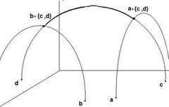
Figure 1.

1.2. Genus zero case

In this case we consider that the hyperbolic manifold $M$ is the hyperbolic space $H^{3}$ with Riemann-sphere as its boundary at infinity. For this case we have

Proposition 1.2.1.

For $a,b,c$ and $d$ in $\mathbb{P}^{1}(\mathbb{C})$, denote by $w_{(a)-(b)}$ a meromorphic function on $\mathbb{P}^{1}(\mathbb{C})$ with the divisor $(a)-(b)$. Then we have

(1.2.1) $$\log\biggm{|}\frac{w_{(a)-(b)}(c)}{w_{(a)-(b)}(d)}\biggm{|}=-ordist(a\ast\{c,d\},b\ast\{c,d\})$$

and

(1.2.2) $$\arg\frac{w_{(a)-(b)}(c)}{w_{(a)-(b)}(d)}=-\psi_{\{c,d\}}(a,b)$$

Proof.

Mobius transformations preserve hyperbolic distance and angel. Then both sides of (1.2.1) and (1.2.2) are invariant under these transformations. Hence it suffices to consider the case when $(a,b,c,d)=(z,1,0,\infty)$ in $\mathbb{P}^{1}(\mathbb{C})$. Then the geodesic $\{a,b\}=\{0,\infty\}$ is the $y$ semi-axis in $(z,y)=(z_{1}+iz_{2},y)$ coordinate for $H^{3}$ and the geodesics joining the points $a=z$ and $b=1$ normally to this semi-axis are half circles passing from these points with center in $0$ and normal to $\mathbb{C}$ ( Figure 2).

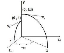
Figure 2.

Then we have $a\ast\{c,d\}=z\ast\{0,\infty\}=(0,|z|)~{}~{},~{}~{}b\ast\{c,d\}=1\ast\{0,\infty\}=(0,1)$ and

$$ordist(a\ast\{c,d\},b\ast\{c,d\})=ordist((0,|z|),(0,1))=-\log|z|.$$

Also from the properties of cross - ratio we have

$$\frac{w_{(a)-(b)}(c)}{w_{(a)-(b)}(d)}=\frac{w_{(z)-(1)}(0)}{w_{(z)-(1)}(\infty)}=z.$$

This gives (1.2.1) directly. To see (1.2.2), we know that angles in $H^{3}$ can be calculated using the Euclidean metric $|dz|^{2}+dy^{2}$ and also the parallel transport along $y$ semi-axis coincides with the Euclidean one. As it’s shown in figure 2 the vectors $v_{1}$ and $v_{2}$ tangent to the geodesics from the points $z$ and $1$, are normal to $\{0,\infty\}$. Hence if we transport (parallel) the vector $v_{2}$ in the point $(0,1)$ to the point $(0,|z|)$ then both vectors are in an Euclidean plane normal to $y$ semi-axis. Then the angel from the vector $v_{1}$ to the vector $v_{2}$ can be calculated via there angels from $z_{1}$ axis. Then we have

$$\psi_{\{0,\infty\}}(z,1)=arg(v_{2})-arg(v_{1})=-arg\frac{w_{(z)-(1)}(0)}{w_{(z)-(1)}(\infty)}.$$

This proves (1.2.2). ∎

The part $w_{(a)-(b)}(c)/w_{(a)-(b)}(d)$ in the proposition above is the classical cross - ratio of four points on the Riemann sphere $\mathbb{P}^{1}(\mathbb{C})$, for which it is convenient to have a special notation

(1.2.3) $$\langle a,b,c,d\rangle:=\frac{w_{(a)-(b)}(c)}{w_{(a)-(b)}(d)}.$$

Theorem 1.2.2.

Let $a,b,c$ and $d$ be in $\mathbb{P}^{1}(\mathbb{C})$. Then we have

$$g((a)-(b),(c)-(d)) =-ordist(a\ast\{c,d\},b\ast\{c,d\})$$

(1.2.4) $$=\log|\langle a,b,c,d\rangle|.$$

Proof.

From the formula (0.0.2) for the Green’s function in the case that the divisors are principal, we have

$$g((a)-(b),(c)-(d)) =\log|w_{(a)-(b)}(c)|^{1}\log|w_{(a)-(b)}(d)|^{-1}$$

$$=\log\biggm{|}\frac{w_{(a)-(b)}(c)}{w_{(a)-(b)}(d)}\biggm{|}.$$

Then from proposition (1.2.1) and notation (1.2.3) we have (1.2.4).∎

1.3. Genus one case

In this case the group that uniformize the hyperbolic 3 - manifold with its boundary at infinity is a cyclic group, and there is a nice explicit formula for the basic Green’s function on the boundary at infinity of 3-manifold; but because we do not use it here we do not want to point to it here. But one can find it in [12]( or for a physical point of view in [14]). Of course the process in the next part can be used for this case too. We have pointed some notes about this case in section 1.4.1.

1.4. Genus$>$1 case and Schottky Groups

Consider the complex projective linear transformations group $\mathrm{PGL}(2,\mathbb{C})$. (i) Kleinian groups. A subgroup $G$ of $\mathrm{PGL}(2,\mathbb{C})$ is called a Kleinian group if $G$ acts on $H^{3}$ properly discontinuously. For a Kleinian group $G$ and a point $p$ in $H^{3}$ lets denote by $G(p)$, the orbit of the point $P$ under the action of $G$. Since $G$ acts on $H^{3}$ Properly discontinuously, $G(p)$ has accumulation points only on $\mathbb{P}^{1}(\mathbb{C})$. They are independent of the choice of the reference point $p$ and are called the limit set of $G$, which is denoted by $\Lambda(G)$. Equivalently, it is the closure of the set of all fixed points of the elements of $G$ other than the identity. $\Lambda(G)$ is the minimal non - empty closed $G$ - invariant set. The complement of the limit set $\mathbb{P}^{1}(\mathbb{C})\setminus\Lambda(G)$ is denoted by $\Omega(G)$ and is called the region of discontinuity of $G$.

The Kleinian group $G$ is called of the first kind if $\Lambda(G)=\mathbb{P}^{1}(\mathbb{C})$ and of the second kind if $\Omega(G)\neq\emptyset$. In the case that $G$ is of the second kind $G$ acts on $\Omega(G)$ properly discontinuously. Therefor in this case $\Omega(G)$ is the maximal open $G$ - invariant subset of $\mathbb{P}^{1}(\mathbb{C})$ where $G$ acts properly discontinuously. The quotient space $\Omega(G)/G$ has the complex structure induced from that of $\Omega(G)$. Thus $\Omega(G)/G$ is a countable union of Riemann surfaces lying at infinity of the complete hyperbolic 3 - manifold $H^{3}/G$. For a torsion free Kleinian group $G$, a manifold $(H^{3}\cup\Omega(G))/G$ possibly with boundary is denoted by $M_{G}$ and is called a Kleinian manifold. The interior $H^{3}/G$ of $M_{G}$ which admits the hyperbolic structure is denoted by $N_{G}$.

(ii) Loxodromic, Parabolic and Elliptic elements. An element $g$ in $\mathrm{PGL}(2,\mathbb{C})$ is called loxodromic if it has exactly two different fixed points in $\mathbb{P}^{1}(\mathbb{C})$. These points are denoted by $z^{+}(g)$ and $z^{-}(g)$ and are called attracting one and repelling one. For any $z_{0}\neq z^{\pm}(g)$ and $h\in\mathrm{PGL}(2,\mathbb{C})$, we have $z^{\pm}(g)=\lim_{n\rightarrow\pm\infty}g^{n},~{}z^{\pm}(g)=z^{\mp}(g^{-1}),~{}z^{\pm}(hgh^{-1})=hz^{\pm}(g)$. If we denote by $q(g)$ the eigenvalue of $g$ on the complex tangent space to $z^{+}(g)$ then there is a local coordinate for $\mathbb{P}^{1}(\mathbb{C})$ that in this coordinate $g$ is represented by $\left(\begin{array}[]{cc}q(g)&0\\ 0&1\end{array}\right)$. For this reason $q(g)$ is called the multiplier of $g$, and we have $|q(g)|<1$, $q(g)=q(g^{-1})=q(hgh^{-1})$. Also by definition $g$ is called a parabolic element if it has precisely one fixed point in $\mathbb{P}^{1}(\mathbb{C})$, and elliptic if it has fixed points in $H^{3}$. In fact an elliptic element fixes all points of a geodesic in $H^{3}$ joining two fixed points in $\mathbb{P}^{1}(\mathbb{C})$. For a loxodromic or elliptic element $g$ the geodesic joining two fixed points in $\mathbb{P}^{1}(\mathbb{C})$ is called axis of $g$. An element is elliptic if and only if it has finite order, then elliptic elements cause a singularity in $N_{G}$. For this reason we consider Kleinian groups without elliptic elements. This means that the group is torsion free or equivalently acts freely on $H^{3}$.

(iii) Schottky groups. A finitely generated, free and purely loxodromic Kleinian group is called a Schottky group. Purely loxodromic means, all elements except the identity are loxodromic. For such a group $\Gamma$ the number of a minimal set of generators is called the genus of $\Gamma$. A marking for a Schottky group $\Gamma$ of genus $p$ by definition is a family of $2p$ open connected domains $D_{1},...,D_{2p}$ in $\mathbb{P}^{1}(\mathbb{C})$ and a family of generators $g_{1},...,g_{p}\in\Gamma$ with the following properties. For $i=1,...,p$

a) The boundary $C_{i}$ of $D_{i}$ is a Jordan curve homeomorphic to $S^{1}$ and closures of $D_{i}$ are pairwise disjoint.

b) $g_{i}(C_{i})\subseteq C_{p+i}$ and $g_{i}(D_{i})\subset\mathbb{P}^{1}(\mathbb{C})\setminus D_{p+i}$.

We say that a marking is classical, if all $C_{i}$ are circles. It is known that every Schottky group admits a marking. In fact each Schottky group admit infinitely many marking but there are some Schottky groups for which no classical marking exists.

(iv) $\Gamma$ - invariant sets of the Schottky groups and there quotient spaces. A Schottky group $\Gamma$ is a Kleinian group, then it acts on $H^{3}$ properly discontinuously. This action is free too. Then the quotient space $N_{\Gamma}=H^{3}/\Gamma$ has a complete hyperbolic 3-manifold structure this means that it is a non-compact Riemann space of constant curvature -1. Topologically, If $\Gamma$ is of genus $p$ then $N_{\Gamma}=H^{3}/\Gamma$ is the interior of a handlebody of genus $p$.

Now lets consider the marking $\{~{}D_{1},...,D_{2p}~{};~{}g_{1},...,g_{p}~{}\}$ for the Schottky group $\Gamma$ of genus $p$ and put

(1.4.1) $$X_{\Gamma}:=\mathbb{P}^{1}(\mathbb{C})\setminus\bigcup_{i=1}^{p}(D_{i}\cup{\bar{D}}_{p+i}),\hskip 14.22636pt\Omega(\Gamma):=\bigcup_{g\in\Gamma}g(X_{\Gamma}).$$

The set $\Omega(\Gamma)$ is the region of discontinuity of $\Gamma$ and $X_{\Gamma}$ is a fundamental domain for the action of $\Gamma$ on $\mathbb{P}^{1}(\mathbb{C})$. Then $\Gamma$ acts on $\Omega(\Gamma)$ freely and properly discontinuously. So the quotient space $S_{\Gamma}=\Omega(\Gamma)/\Gamma$ is a complex Riemann surface of genus $p$. All compact Riemann surfaces can be obtained in this way ( see [8]) and every compact Riemann surface admits infinitely many different Schottky covers.

The Cayley graph of a Schottky group $\Gamma$ of genus $p$ is an infinite tree with multiplicity of $2p$ at each vertex. $\Gamma$ is free, then this tree is without loops and each path between two points is unique. Now, by the definition of a marking for $\Gamma$, each generator $g_{i}$ takes $X_{\Gamma}$ to the inside of $C_{p+i}$ and again the generator $g_{j}$ takes this part to the inside of the second copy of $C_{p+j}$ inside $C_{p+i}$. This means that for each element $g$ in $\Gamma$ we can associate a path in the Cayley graph that the points of $X_{\Gamma}$ moves along that path on a tubular neighborhood. This express the action of $\Gamma$ on the set $\Omega(\Gamma)$ ( Figure 3 illustrating this for the case $p=2$ ).

Figure 3.

We can consider the Riemann surface $S_{\Gamma}$ as the boundary at infinity of the manifold $N_{\Gamma}$ by identifying the points of $S_{\Gamma}$ with the points of the set of equivalence classes of unbounded ends of oriented geodesics in $N_{\Gamma}$ modulo the relation ”distance=0”.

By the definition of the limit set for a Kleinian group, the complement

(1.4.2) $$\Lambda(\Gamma):=\mathbb{P}^{1}(\mathbb{C})\setminus\Omega(\Gamma)$$

is the limit set of $\Gamma$. For the cyclic Schottky groups ( of genus 1 ) the limit set $\Lambda(\Gamma)$ consists of two points which can be chosen as $0,\infty$, but for genus$\geq 2$ this set is an infinite Cantor set ( see [18]).

Lets consider the irreducible left - infinite words like $\bar{h}=...h_{i}^{\varepsilon_{i}}...h_{0}^{\varepsilon_{0}}$. Where $h_{i}\in\{g_{1},...,g_{p}\}$, $\varepsilon_{i}=\pm 1$, and $z_{0}$ is a point in the fundamental domain $X_{\Gamma}$. And put

(1.4.3) $$z^{+}(\bar{h})=\lim_{i\rightarrow+\infty}h_{i}^{\varepsilon_{i}}...h_{0}^{\varepsilon_{0}}(z_{0})$$

This is a well defined point of $\Lambda(\Gamma)$ and is independent of the point $z_{0}$. Since $\Gamma$ is a free group, the map $\bar{h}\mapsto z^{+}(\bar{h})$ establishes a bijection as following

Irreducible left - infinite words in $g_{i}$

$\updownarrow$

Ends of the Cayley graph of $\Gamma$, $\{g_{i}\}$

$\updownarrow$

Points of $\Lambda(\Gamma).$

Denote by $a(\Gamma)$ the Hausdorff dimension of the set $\Lambda(\Gamma)$. It can be characterized as the convergence abscissa of any Poincare series

(1.4.4) $$\sum_{g\in\Gamma}\biggm{|}\frac{dg(z)}{dz}\biggm{|}^{s}.$$

Where $z$ is any coordinate function on $\mathbb{P}^{1}(\mathbb{C})$ with a zero and a pole in $\Omega(\Gamma)$. For $s\in\mathbb{C}$ that Re$(s)>a(\Gamma)$, this series converges uniformly on compact subsets of $\Omega(\Gamma)$. Generally we have $0<a(\Gamma)<2$ (See [3]). In the next section we will consider $a(\Gamma)<1$ to have the convergency of some infinite products defining some $\Gamma$ - automorphic functions. This class of Schottky groups was characterized by Bowen [3] in following way: $a(\Gamma)<1$ if and only if $\Gamma$ admits a rectifiable invariant quasi-circle (which then contains $\Lambda(\Gamma)$ ).

Choose marking for $\Gamma$ of genus $p$ and denote by $a_{i}$ the image of $C_{i}$ in $S_{\Gamma}$ with induced orientation. Also for $i=1,...,p$ choose the points $x_{i}$ in $C_{i}$ and denote by $b_{i}$ the images in $S_{\Gamma}$ of oriented pathes from $x_{i}$ to $g_{i}(x_{i})$ lying in $X_{\Gamma}$. These images are obviously closed paths and we can choose them in such a way that they don’t intersect. If we denote the classes of these pathes in 1- homology group $H_{1}(S_{\Gamma},\mathbb{Z})$ by the same notations, then the set $\{a_{i},b_{j}\}$ form a canonical basis of this group i.e. for all $i=1,...,p$ we have

(1.4.5) $$(a_{i},a_{j})=(b_{i},b_{j})=0~{},~{}(a_{i},b_{j})=\delta_{ij}.$$

Moreover the kernel of the map $H_{1}(S_{\Gamma},\mathbb{Z})\longrightarrow H_{1}(M_{\Gamma},\mathbb{Z})$ which is induced by the inclusion $S_{\Gamma}\hookrightarrow M_{\Gamma}$ is generated by the classes $a_{i}$.

1.4.1. Differentials of the first kind

Lets consider the cyclic Schottky group $\Gamma=<qz>$, for $q\in\mathbb{C}^{*}$, $|q|<1$. In this case $\Lambda(\Gamma)=\{0,\infty\}$ and consequently $\Omega(\Gamma)=\mathbb{C}^{*}$. Then a differential of the first kind on $\Omega(\Gamma)=\mathbb{C}^{*}$ can be written as

(1.4.6) $$\omega=d\log z=d\log\frac{w_{(0)-(\infty)}(z)}{w_{(0)-(\infty)}(z_{0})}=d\log\langle 0,\infty,z,z_{0}\rangle.$$

where $z_{0}$ is any point $\neq 0,\infty$. And for $d\log q^{n}z=d\log z$, this differential determines a differential of the first kind on $S_{\Gamma}$. In general case for a Schottky group $\Gamma$ of genus $p$ we can make a differential of the first kind $\omega_{g}$ for any $g\in\Gamma$ on $\Omega(\Gamma)$ and $S_{\Gamma}$ by an appropriate averaging of this formula. Lets consider a marking for $\Gamma$ and Denote by $C(|g)$ a set of representatives of $\Gamma/(g^{\mathbb{Z}})$; by $C(h|g)$ a similar set for $(h^{\mathbb{Z}})\setminus\Gamma/(g^{\mathbb{Z}})$; and by $S(g)$ the conjugacy class of $g$ in $\Gamma$. Then for any $z_{0}\in\Omega(\Gamma)$ we have

Proposition 1.4.1.

(a) If $a(\Gamma)<1$, the following series converges absolutely for $z\in\Omega(\Gamma)$ and determines (the lift to $S_{\Gamma}$ of ) a differential of the first kind on $S_{\Gamma}$:

(1.4.7) $$\omega_{g}=\sum_{h\in C(|g)}d\log\langle h(z^{+}(g)),h(z^{-}(g)),z,z_{0}\rangle.$$

This differential does not depend on $z_{0}$, and depends on $g$ additively. Also If the class of $g$ is primitive ( i.e. non - divisible in H:$=\Gamma/[\Gamma,\Gamma]$ ), $\omega_{g}$ can be rewritten as following

(1.4.8) $$\omega_{g}=\sum_{h\in S(g)}d\log\langle z^{+}(h),z^{-}(h),z,z_{0}\rangle.$$

(b) If $g_{i}$ form a part of the marking of $\Gamma$, and $a_{i}$ are the homology classes described before, we have

(1.4.9) $$\int_{a_{i}}\omega_{g_{j}}=2\pi i\delta_{ij}.$$

It follows that the map $g$ mod $[\Gamma,\Gamma]\mapsto\omega_{g}$ embeds $H$ as a sublattice in the space of all differentials of the first kind.

(c) Denote by $\{b_{j}\}$ the complementary set of homology classes in $H_{1}(S_{\Gamma},\mathbb{Z})$ as in before. Then we have for $i\neq j$, with an appropriate choice of logarithm branches:

(1.4.10) $$\tau_{ij}:=\int_{b_{i}}\omega_{g_{j}}=\sum_{h\in C(g_{i}|g_{j})}\log\langle z^{+}(g_{i}),z^{-}(g_{i}),h(z^{+}(g_{j})),h(z^{-}(g_{j}))\rangle$$

And

(1.4.11) $$\tau_{ii}=\log q(g_{i})+\sum_{h\in C_{0}(g_{i}|g_{i})}\log\langle z^{+}(g_{i}),z^{-}(g_{i}),h(z^{+}(g_{i})),h(z^{-}(g_{i}))\rangle$$

where $C_{0}(g_{i}|g_{i})$ is $C(g_{i}|g_{i})$ without the identity class.

Proof.

For the proofs, see [12] and [13]. Notice that our notation here slightly differs from [12]; in particular, $\tau_{ij}$ here corresponds to $2\pi i\tau_{ij}$ of [12].∎

1.4.2. Differentials of the third kind and Green’s functions

Lets consider the points $a$ and $b$ in $X_{\Gamma}$ the fundamental domain of $\Gamma$ and put $\nu_{(a)-(b)}=\sum_{h\in\Gamma}d\log\langle a,b,h(z),h(z_{0})\rangle$. Then assuming $a(\Gamma)<1$, we see that this series absolutely converges and because it’s $\Gamma$ - automorphic it gives us a differential of the third kind on $S_{\Gamma}$ with residues $\pm 1$ at the images of $a,b$ in $S_{\Gamma}$. Moreover, since both points $a,b$ are out of the circles $C_{i}$, its $a_{i}$ - periods vanish. Now, if we consider the linear combination $\nu_{(a)-(b)}-\sum_{j=1}^{p}X_{j}(a,b)\omega_{g_{j}}$ with real coefficients $X_{j}$, then it will have pure imaginary $a_{i}$ - periods and If we find real coefficients $X_{j}$ so that the real part of $b_{i}$ - periods of the form

(1.4.12) $$\omega_{(a)-(b)}=\nu_{(a)-(b)}-\sum_{j=1}^{p}X_{j}(a,b)\omega_{g_{j}}$$

vanish, we will be able to use this differential in order to calculate conformally invariant Green’s functions. The set of the equations for calculating the coefficients $X_{j}(a,b)$ are as following

(1.4.13) $$\sum_{j=1}^{p}X_{j}(a,b)Re\tau_{ij}=Re\int_{b_{i}}\nu_{(a)-(b)}=\sum_{h\in S(g_{i})}\log|\langle a,b,z^{+}(h),z^{-}(h)\rangle|$$

for $i=1,...,p$. The parts $Re\tau_{ij}$ are calculated by means of formula (1.4.10) and (1.4.11), and $b_{i}$ - periods of $\nu_{(a)-(b)}$ are given in [12].

Now if we denote the points $a,b,c$, and $d$ in $S_{\Gamma}$ and their images in the fundamental domain $X_{\Gamma}$ by the same notations, then we have

$$Re\int_{d}^{c}\nu_{(a)-(b)}=\sum_{h\in\Gamma}\log\mid\langle a,b,h(c),h(d)\rangle\mid,~{}Re\int_{d}^{c}\omega_{g_{j}}=\sum_{h\in S(g_{j})}\log\mid\langle z^{+}(h),z^{-}(h),c,d\rangle\mid$$

And finally we have the Green’s function on $S_{\Gamma}$ as following

$$g((a)-(b),(c)-(d)) =Re\int_{d}^{c}\omega_{(a)-(b)}$$

$$=\sum_{h\in\Gamma}\log\mid\langle a,b,h(c),h(d)\rangle\mid$$

(1.4.14) $$-\sum_{j=1}^{p}X_{j}(a,b)\sum_{h\in S(g_{j})}\log\mid\langle z^{+}(h),z^{-}(h),c,d\rangle\mid.$$

2. Two boundary component case

All hyperbolic Riemann surfaces are uniformized by Fuchsian groups. Also Fuchsian groups act on hyperbolic space by Poincare extension and uniformize some hyperbolic 3-manifolds with two boundaries at infinity with the same genera. But they do not uniformize all such manifolds; In fact they are uniformized by an extension of Fuchsian groups that are called Quasi-Fuchsian groups. In this chapter first we intend to extend the method in previous chapter to fuchsian groups and then for Quasi-fuchsian groups.

Consider hyperbolic plane $H^{2}$ with the upper half plane model and coordinate $z=x+iy\in\mathbb{C}$ with $y>0$, equipped by the hyperbolic distance function corresponding to the metric

(2.0.1) $$ds^{2}=\frac{|dz|^{2}}{y^{2}}$$

of the constant curvature -1. The geodesics in this model are vertical half-lines $x=constant$ and vertical half-circles orthogonal to the line at infinity $\mathbb{R}$ ( i.e, for $y=0$ ).

If we consider the end points of geodesics ( including $\infty$ for the end of vertical half-lines other than the end in $\mathbb{R}$ ) then we can consider circle $\hat{\mathbb{R}}=\mathbb{R}\cup\{\infty\}$ ( or $\mathbb{P}^{1}(\mathbb{R})=S^{1}$ in unit disc model ) as boundary at infinity of $H^{2}$.

2.1. Fuchsian Groups

Each subgroup $F$ of $PGL(2,\mathbb{R})$, the general projective linear group over $\mathbb{R}$, that acts freely and properly discontinuously on $H^{2}$ is called a Fuchsian group. Similar to the Kleinian groups the limit set $\Lambda(F)$ and the region of discontinuity $\Omega(F)$ are defined but in $\hat{\mathbb{R}}$, the boundary at infinity of $H^{2}$. And the properties are similar to them. Also similar to the loxodromic elements, a hyperbolic element is an element $h\in PGL(2,\mathbb{R})$ with two fixed points $z^{\pm}(h)$ in $\hat{\mathbb{R}}$. For a Fuchsian group $F$ the quotient space $H^{2}/F$ is a hyperbolic Riemann surface possibly with boundary $\Omega(F)/F$ ( If $\Omega(F)\neq\emptyset$ ).

Let $F$ be a Fuchsian group such that $S=H^{2}/F$ is a compact Riemann surface with the genus $p>1$. Then $F$ is a purely hyperbolic group of finite order $2p$ (for example see [9]). Lets denote by $f_{i}$ the generators of $F$ and by $Fix(f_{i})=\{z^{\pm}(f_{i})\}$ the fixed point set of $f_{i}$. Also consider that $P$ is the fundamental polygon of $F$ with $a_{1},b_{1},a^{\prime}_{1},b^{\prime}_{1},\ldots,b^{\prime}_{p}$ as it’s sides, such that $f_{i}(a_{i})=a^{\prime}_{i}$ and $f_{p+i}(b_{i})=b^{\prime}_{i}$ for $i=1,\ldots,p$. We represent $P$ as following:

(2.1.1) $$P=a_{1}(x_{1})b_{1}(y_{1})a^{\prime}_{1}(x^{\prime}_{1})b^{\prime}_{1}(y^{\prime}_{1})\ldots a^{\prime}_{p}(x^{\prime}_{p})b^{\prime}_{p}(y^{\prime}_{p})$$

Where $x_{i},x^{\prime}_{i},y_{i}$ and $y^{\prime}_{i}$ are the intersection points of $a_{i}$ and $b_{i}$, $a_{i}^{\prime}$ and $b_{i}^{\prime}$ and so on. Now we have

$$\pi_{1}(S)\simeq F=\langle\{f_{i}\ ;i=1,\ldots,2p\};\prod_{1}^{p}[f_{i},f_{p+i}]=I\rangle$$

And also ( See for example [9]).

$$H_{1}(S,\mathbb{Z})=\frac{\pi_{1}(S)}{\langle\left\{aba^{-1}b^{-1}|a,b\in\pi_{1}(S)\right\}\rangle}=\mathbb{Z}\oplus\ldots\oplus\mathbb{Z}\qquad(2p~{}~{}times)$$

If we denote by ${\overline{a}}_{i}$ and ${\overline{b}}_{i}$ the images of $a_{i}$ and $b_{i}$ in $S$, then $\{{\overline{a}}_{i},{\overline{b}}_{j}\}$ generate $H_{1}(S,\mathbb{Z})$.

2.2. Extension of Fuchsian group on $H^{3}$

$F$ acts similarly, freely and properly discontinuously on lower half plane $-H^{2}$ of $\mathbb{C}$ too, and $-H^{2}$ is $F$-invariant. Lets denote by $F$ the Poincare extension of $F$ on $H^{3}$ too (see [15] or [18]). By this extension $F$ can be considered as a Kleinian group. And we have

$$N_{F}=\frac{H^{3}}{F}\cong\frac{H^{2}}{F}\times(0,1)=S\times(0,1)\qquad and\qquad F=\pi_{1}(N_{F})=\pi_{1}(S)$$

(See [15]). And $N_{F}$ has a hyperbolic structure, [16].

2.3. F invariants

We know that $\Lambda(F)$ the limit point set of $F$ is $\mathbb{\hat{R}}$ ( $S^{1}$ in unit disc model ), [3]. Then as a Kleinian group $\Lambda(F)=\mathbb{\hat{R}}\subset\hat{\mathbb{C}}$ and the region of discontinuity of $F$ considering as a Kleinian group is

(2.3.1) $$\Omega(F)=\mathbb{\hat{C}}\backslash\Lambda(F)=\mathbb{\hat{C}}\backslash\mathbb{\hat{R}}=-H^{2}\cup H^{2}$$

And also the Kleinian manifold is

(2.3.2) $$M_{F}=\frac{H^{3}\cup(-H^{2}\cup H^{2})}{F}=S\times[0,1].$$

Now because $S$ is compact then $\partial S=\emptyset$. Consequently $N_{F}$ is a hyperbolic 3 - manifold with two compact boundary component at infinity $S_{0}=H^{2}/F=S\times\{0\}$ and $S_{1}=-H^{2}/F=S\times\{1\}$ with the same genus $p$.

2.4. Coding of the points of $\Lambda(F)$ and the Geodesics

For convenience and having a simple intuition lets consider the unit disc model for $H^{2}$ in this section. We can code points of $\Lambda(F)=S^{1}$ and geodesics with beginning and end points on $\Lambda(F)=S^{1}$ as following:

Lets mark semicircles including sides of P by $c_{1},...,c_{4p}$ in the counter clockwise direction around $S^{1}$ and put $g_{1}=f_{1},g_{2}=f_{p+1},g_{3}=f^{-1}_{1},g_{4}=f^{-1}_{p+1},g_{5}=f_{2},g_{6}=f_{p+2},g_{7}=f_{2}^{-1},g_{8}=f_{p+2}^{-1}$, and so on. In general for $k=0,...,p-1$, $g_{4k+1}=f_{k+1},g_{4k+2}=f_{p+k+1},g_{4k+3}=f^{-1}_{k+1},g_{4k+4}=f^{-1}_{p+k+1}$. And label end points of $c_{i}$ on $S^{1}$ by $P_{i}$ and $Q_{i+1}$ ( with $Q_{4p+1}=Q_{1}$ ) with $P_{i}$ occurring before $Q_{i+1}$ in the counter clockwise direction, ( See figure 4 ). And define

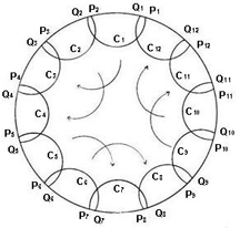
Figure 4.

$$f_{F}:S^{1}\rightarrow S^{1}$$

$$f_{F}(x)=g_{i}(x)\hskip 14.22636ptif\hskip 14.22636ptx\in[P_{i},P_{i+1})$$

Then $f_{F}$ is a well defined map and is called a Markov map related to the Fuchsian group $F$. We have the following lemma

Lemma 2.4.1.

The map $f_{F}$ and the group $F$ are orbit equivalent on $S^{1}$, namely except for the pairs $(Q_{i},g_{i-1}Q_{i})$, for $i=1,2,...,4p$; for each x,y in $S^{1}$, $x=f(y)$ for some $f$ in $F$ if and only if there exists nonnegative integers $n,m$ such that $f_{F}^{n}(x)=f_{F}^{m}(y)$.

Proof.

( See [4]).∎

Now label each arc $[P_{i},P_{i+1})$ by $g_{i}$, and for each element $x$ in $S^{1}$ put $x=(...,x_{2},x_{1},x_{0})$. Where the component $x_{n}$ is the label of the segment to which $f_{F}^{n}(x)$ belongs. We know that for each generator $f_{i}$ of $F$, the fixed point $Z^{+}(f_{i})$ is in the circle $a_{i}^{\prime}\cup(-a_{i}^{\prime})$ and $Z^{-}(f_{i})$ is in $a_{i}\cup(-a_{i})$ then from the definition of Markov map we have

(2.4.1) $$Z^{+}(f_{i})=(...,f_{i}^{-1},f_{i}^{-1},f_{i}^{-1})\qquad and\qquad Z^{-}(f_{i})=(...,f_{i},f_{i},f_{i})$$

Next, if $\{x,y\}$ be a geodesic with the beginning point $x\in S^{1}$ and end point $y=(...,y_{2},y_{1},y_{0})\in S^{1}$ then put

(2.4.2) $$\{x,y\}=(...,x_{2},x_{1},x_{0},y_{0}^{-1},y_{1}^{-1},y_{2}^{-1},...).$$

Now for each $h\in F$ let $\gamma_{h}=\{z^{+}(h),z^{-}(h)\}$ show the geodesic arc between $z^{+}(h)$ and $z^{-}(h)$ (the axis of $h$) and ${\overline{\gamma}}_{h}$ the image of $\gamma_{h}$ in $N_{F}$. Then we have the following geodesics in $N_{F}$

• Closed geodesics: a geodesic in $N_{F}$ is closed if and only if it’s the projection of the axis of a hyperbolic element in $F$,

• Images of the geodesics with beginning and end points in $\Lambda(F)$,

• Geodesics with beginning points in $\partial N_{F}$ that are limit cycle to ${\overline{\gamma}}_{f_{i}}$, for a generator $f_{i}$ of $F$,

• Geodesics with beginning and end points in $S_{0}$ or $S_{1}$.,

• Geodesics with beginning point in $S_{0}$ and end point in $S_{1}$ and vis versa.

2.5. Schottky groups associated to the Fuchsian groups

For the Riemann surface $S$ and associated Fuchsian group $F$ as above let $N$ be the smallest normal subgroup of $F$ including $f_{i}$ for $i=p+1,...,2p$. Then it’s obvious that the factor group $F/N$ is a free group generated by $p$ generators. If we consider the covering $\tilde{S}\rightarrow S$ associated to $N$, then from normality of $N$ the group of deck transformations of this cover is $F/N$ and according to the classical Koebe uniformization theorem [10]( see also [7])there is a planar region $\Omega\subset\mathbb{\hat{C}}$ that is a region of discontinuity of a Schottky group $\Gamma=<\gamma_{1},\gamma_{2},...,\gamma_{p}>$ and $F/N\simeq\Gamma$. $\tilde{S}$ is covering isomorphic to $\Omega=\Omega(\Gamma)$ and for coverings $J:H^{2}\longrightarrow\Omega(\Gamma)$, $\pi_{\Gamma}:\Omega(\Gamma)\longrightarrow\Omega(\Gamma)/\Gamma$ and $\pi_{F}:H^{2}\longrightarrow H^{2}/F$ we have $\pi_{\Gamma}\circ J=\pi_{F}$ i.e. the following diagram is commutative

$H^{2}\hskip 14.22636pt\overset{J}{\longrightarrow}\hskip 14.22636pt\Omega(\Gamma)$

$\pi_{F}\searrow\hskip 19.91692pt\swarrow\pi_{\Gamma}$

$S$

Also we have $J\circ f_{i}=\gamma_{i}\circ J$ for $i=1,...,p$ and $J\circ f=J$ for each $f$ in $N$ and each mappings is complex-analytic covering and $\Gamma$ is uniquely determined to within conjugation in $PGL(2,\mathbb{C})$ [19].

For an extension of $J$ to a set some more than $H^{2}$ that we need it in the later computations, lets denote by $F_{0}$ the free subgroup of $F$ generated by $f_{1},...,f_{p}$. We know that $\Lambda(F_{0})$ is a subset of $\Lambda(F)$. $\Lambda(F_{0})$ is $F_{0}$ invariant and is out of the closer of the fundamental domain of $F_{0}$, then all points of $\Lambda(F_{0})$ are in only the circles $C_{i}$ that are related to the generators of $F_{0}$ and their inverses. This shows that the coding of each point in $\Lambda(F_{0})$ includes only the generators of $F_{0}$ and their inverses. Also since each generator of $F$ like $f$ is an isometry of $H^{2}$, it’s a composition of two reflections, then $f(x)$ is not in the isometry circle of $f^{-1}$ for each point $x$ in $S^{1}$. Then by the definition of the Markov map $f_{F}$ all the codings of the points of $S^{1}$ are irreducible. This means that each point $x$ in $\Lambda(F_{0})$ can be coded by the irreducible formal combination $x=(...,f_{i_{2}}^{\epsilon_{i_{2}}},f_{i_{1}}^{\epsilon_{i_{1}}},f_{i_{0}}^{\epsilon_{i_{0}}})$ for $i_{j}\leq p$. This Fuchsian coding is suitable for expressing geodesics in $N_{F}$ or $S_{F}$ when the beginning and end points of the geodesics are in $\Lambda(F_{0})$ and also can be used for extending the map $J$ on $\Lambda(F_{0})$ and maybe on some more.

Now we want to extend $J$ to $H^{2}\cup\Lambda(F_{0})$ ( onto $\overline{\Omega(\Gamma)}=\hat{\mathbb{C}}$ ). For this, we know that each element of $\Lambda(\Gamma)$ can be coded by the infinite words $z=...\gamma_{i_{2}}^{\epsilon_{i_{2}}}\gamma_{i_{1}}^{\epsilon_{i_{1}}}\gamma_{i_{0}}^{\epsilon_{i_{0}}}(z_{0})$ for a constant $z_{0}$ in $\Omega(\Gamma)$ and $\epsilon_{i}=\pm 1$. Similarly, since $F_{0}$ is free and purely loxodromic group then it’s a Schottky group too and we can use Schottky coding for it too. For conveniences in some proofs we will use Schottky codings for the points of $\Lambda(F_{0})$. Then each point $x$ in $\Lambda(F_{0})$ can be coded by the infinite words $x=...f_{i_{2}}^{\epsilon_{i_{2}}}f_{i_{1}}^{\epsilon_{i_{1}}}f_{i_{0}}^{\epsilon_{i_{0}}}(x_{0})$ for $i_{j}\leq p$ and a constant point $x_{0}$ in $\Omega(F_{0})\subset\hat{\mathbb{C}}$ ( also $H^{2}\subset\Omega(F_{0})$ ). Then we can consider $x_{0}$ in $\Omega(F_{0})\cap H^{2}$ such that $z_{0}=J(x_{0})$. Also from (2.4.1) and using the properties of a loxodromic element and invariance of the limit set under $F$ ( or $F_{0}$ ) it is not hard to show that on $\Lambda(F_{0})$ we have the following relation between Fuchsian and Schottky coding

$$...f_{i_{k}}^{\epsilon_{i_{k}}}...f_{i_{1}}^{\epsilon_{i_{1}}}f_{i_{0}}^{\epsilon_{i_{0}}}f_{i_{k}}^{\epsilon_{i_{k}}}... f_{i_{1}}^{\epsilon_{i_{1}}}f_{i_{0}}^{\epsilon_{i_{0}}}(x_{0})=Z^{+}(f_{i_{k}}^{\epsilon_{i_{k}}}...f_{i_{1}}^{\epsilon_{i_{1}}}f_{i_{0}}^{\epsilon_{i_{0}}})$$

(2.5.1) $$=(...,f_{i_{0}}^{-\epsilon_{i_{0}}},...,f_{i_{k-1}}^{-\epsilon_{i_{k-1}}},f_{i_{k}}^{-\epsilon_{i_{k}}},f_{i_{0}}^{-\epsilon_{i_{0}}},...,f_{i_{k-1}}^{-\epsilon_{i_{k-1}}},f_{i_{k}}^{-\epsilon_{i_{k}}})$$

And also this is true for repelling points too because of the relation $Z^{-}(f)=Z^{+}(f^{-1})$ for each $f$ in $F$ . Now, lets put

(2.5.2) $$J(...f_{i_{2}}^{\epsilon_{i_{2}}}f_{i_{1}}^{\epsilon_{i_{1}}}f_{i_{0}}^{\epsilon_{i_{0}}}(x_{0}))=...\gamma_{i_{2}}^{\epsilon_{i_{2}}}\gamma_{i_{1}}^{\epsilon_{i_{1}}}\gamma_{i_{0}}^{\epsilon_{i_{0}}}(z_{0})$$

in other words, by the definition of infinite words, the continuity of $J$ and the relation $J\circ f(x)=\gamma\circ J(x)$ on $H^{2}$

$$J(...f_{i_{2}}^{\epsilon_{i_{2}}}f_{i_{1}}^{\epsilon_{i_{1}}}f_{i_{0}}^{\epsilon_{i_{0}}}(x_{0})) =J(\lim_{j\rightarrow\infty}f_{i_{j}}^{\epsilon_{i_{j}}}...f_{i_{2}}^{\epsilon_{i_{2}}}f_{i_{1}}^{\epsilon_{i_{1}}}f_{i_{0}}^{\epsilon_{i_{0}}}(x_{0}))$$

$$=\lim_{j\rightarrow\infty}Jf_{i_{j}}^{\epsilon_{i_{j}}}...f_{i_{2}}^{\epsilon_{i_{2}}}f_{i_{1}}^{\epsilon_{i_{1}}}f_{i_{0}}^{\epsilon_{i_{0}}}(x_{0})$$

$$=\lim_{j\rightarrow\infty}\gamma_{i_{j}}^{\epsilon_{i_{j}}}...\gamma_{i_{2}}^{\epsilon_{i_{2}}}\gamma_{i_{1}}^{\epsilon_{i_{1}}}\gamma_{i_{0}}^{\epsilon_{i_{0}}}(J(x_{0}))$$

$$=...\gamma_{i_{2}}^{\epsilon_{i_{2}}}\gamma_{i_{1}}^{\epsilon_{i_{1}}}\gamma_{i_{0}}^{\epsilon_{i_{0}}}(z_{0})$$

Then the map $J:\Lambda(F_{0})\rightarrow\Lambda(\Gamma)$ is well defined and onto. Also from (2.5.1) we see that we can explain $J$ and consequently the functions ( spatially Green’s function ) on $S_{0}$ by the Fuchsian coding, when these functions are expressed via this map.

For each point $x$ in $\Lambda(F_{0})$ and element $f$ in $F_{0}$ equivalent to $\gamma$ (i.e. $f=f_{i_{k}}^{\epsilon_{i_{k}}}...f_{i_{1}}^{\epsilon_{i_{1}}}f_{i_{0}}^{\epsilon_{i_{0}}}\sim\gamma=\gamma_{i_{k}}^{\epsilon_{i_{k}}}...\gamma_{i_{1}}^{\epsilon_{i_{1}}}\gamma_{i_{0}}^{\epsilon_{i_{0}}}$, where $i_{j}\leq p$ and $f_{i}$ is replaced by $\gamma_{i}$ and vice versa ) we have

$$J\circ f(...f_{i_{2}}^{\epsilon_{i_{2}}}f_{i_{1}}^{\epsilon_{i_{1}}}f_{i_{0}}^{\epsilon_{i_{0}}}(x_{0}))=\gamma\circ J(...f_{i_{2}}^{\epsilon_{i_{2}}}f_{i_{1}}^{\epsilon_{i_{1}}}f_{i_{0}}^{\epsilon_{i_{0}}}(x_{0}))$$

Then $J\circ f=\gamma\circ J$ and $J(z^{\pm}(f))=z^{\pm}(\gamma)$.

2.6. Automorphic Functions on $S_{0}$

Let $F_{0}$ be the free group generated by $f_{1},...,f_{p}$ and $D=\Sigma m_{x}(x)$ be a divisor with support $|D|$ in $H^{2}$. Put $D_{0}:=\Sigma m_{x}(Jx)$ and again lets denote by $w_{A}$ a meromorphic function on $\mathbb{P}^{1}(\mathbb{C})$ with the divisor $A$, and for an element $x_{0}$ in $H^{2}\backslash\bigcup_{f\in F_{0}}f(|D|)$ define:

(2.6.1) $$W_{D,x_{0}}(x)=\prod_{f\in F_{0}}\frac{w_{D_{0}}(Jf(x))}{w_{D_{0}}(Jf(x_{0}))}.$$

Theorem 2.6.1.

For the Schottky group $\Gamma$ associated to the Fuchsian group $F$, if $a(\Gamma)<1$, then the product (2.6.1) converges absolutely and uniformly on any compact subset of $H^{2}$, after deleting a finite number of factors that may have a pole or zero on this subset.

Proof.

Let $K$ be a compact subset of $H^{2}$. Since $F$ acts on $H^{2}$ properly discontinuously the set $K_{F_{0}}=\{f\in F_{0}|f(K)\cap|D|\neq\emptyset\}$ is finite. If we delete the set $K_{F_{0}}$ from the index set of the product (2.6.1) then for each $f\in F_{0}\setminus K_{F_{0}}$ when $f(x)$ and $f(x_{0})$ lie outside a fixed compact neighborhood of $|D|$ we have

$$\biggm{|}\frac{w_{D_{0}}(Jf(x))}{w_{D_{0}}(Jf(x_{0}))}-1\biggm{|} \leq c|Jf(x)-Jf(x_{0})|=c|\alpha(z)-\alpha(z_{0})|$$

$$\leq\frac{c}{2}|z-z_{0}|\biggm{|}\frac{d\alpha(z)}{dz}+\frac{d\alpha(z_{0})}{dz}\biggm{|}$$

Where $c$ is a constant, $z=J(x)$, $z_{0}=J(x_{0})$ and $f\sim\alpha=\left(\begin{array}[]{cc}a&b\\ c&d\end{array}\right)$ ( and $ad-bc=1$). The last inequality comes from the equality $\frac{1}{|cz+d|^{2}}=|\frac{d\alpha(z)}{dz}|$. Now since $a(\Gamma)<1$ the series

(2.6.2) $$\sum_{\gamma\in\Gamma}\biggm{|}\frac{d\gamma(z)}{dz}\biggm{|}$$

converges uniformly on the compact subsets of $\Omega(\Gamma)$. Then the product (2.6.1) is convergent. ∎

In $W_{D,x_{0}}(x)$, if we change the point $x_{0}$ to $x_{1}$, then we have $W_{D,x_{0}}(x)=C^{x_{1}}_{x_{0}}W_{D,x_{1}}(x)$. Where $C^{x_{1}}_{x_{0}}$ is a nonzero complex number that depends on the points $x_{0}$ and $x_{1}$ and $C^{x_{1}}_{x_{0}}C^{x_{0}}_{x_{1}}=1$. Also, for $f\in F$ and $x\in H^{2}$ we have

$$W_{D,x_{0}}(fx)=\prod_{h\in F_{0}}\frac{w_{D_{0}}(Jh(x_{0})))}{w_{D_{0}}(Jhf^{-1}(x_{0}))}\prod_{h\in F_{0}}\frac{w_{D_{0}}(Jh(x))}{w_{D_{0}}(Jh(x_{0}))}=\mu_{D}(f)W_{D,x_{0}}(x).$$

$\mu_{D}(f)$ is a nonzero complex number multiplicative on $D$ and $f$ and also independent of $x_{0}$. We can see this as following

$$\mu_{D}^{x_{0}}(f)W_{D,x_{0}}(x)=W_{D,x_{0}}(fx)=C^{x_{1}}_{x_{0}}\mu_{D}^{x_{1}}(f)C^{x_{0}}_{x_{1}}W_{D,x_{0}}(x)=\mu_{D}^{x_{1}}(f)W_{D,x_{0}}(x)$$

Then $\mu_{D}^{x_{0}}(f)=\mu_{D}^{x_{1}}(f)$. When $\Gamma$ is a cyclic group $\mu_{D}(f)=1$. This shows that $W_{D,x_{0}}$ is not $F$ automorphic function on $H^{2}$ in general.

Theorem 2.6.2.

a) Lets denote by $C(f|g)$ a set of the representatives of $(f^{n})\backslash F_{0}/(g^{n})$. Then for $f\neq g~{}mod[F_{0},F_{0}]$ in $F_{0}$ we have

$$\mu_{(g(x_{1}))-(x_{1})}(f) =\prod_{h\in F_{0}}\frac{w_{(Jg(x_{1}))-(Jx_{1})}(J(h(x_{0})))}{w_{(Jg(x_{1}))-(Jx_{1})}(J(h\circ f^{-1}(x_{0})))}$$

(2.6.3) $$=\prod_{h\in C(f|g)}\frac{w_{(J(z^{+}(f)))-(J(z^{-}(f)))}(Jh(z^{+}(g)))}{w_{(J(z^{+}(f)))-(J(z^{-}(f)))}(Jh(z^{-}(g)))}$$

And by defining $Q(f):=\langle J(z^{+}(f)),J(z^{-}(f)),J(f(x_{1})),J(x_{1})\rangle$ we have

(2.6.4) $$\mu_{(f(x_{1}))-(x_{1})}(f)=Q(f)\prod_{h\in C_{0}(f|f)}\frac{w_{(J(z^{+}(f)))-(J(z^{-}(f)))}(Jh(z^{+}(f)))}{w_{(J(z^{+}(f)))-(J(z^{-}(f)))}(Jh(z^{-}(f)))}$$

Where $C_{0}(f|f)$ is the set $C(f|f)$ without the identity class.
b) Lets denote by $C(|f)$ a set of representatives of $F_{0}/(f^{n})$ and by $S(f)$ the conjugacy class of $f$ in $F_{0}$. Then for some $x_{1}$ in $H^{2}$ such that $z_{1}=J(x_{1})$ stays in $\Omega(\Gamma)\setminus\Gamma_{\infty}$, we have

$$W_{(f(x_{1}))-(x_{1}),x_{0}}(x) =\prod_{h\in C(|f)}\frac{w_{(Jh(z^{+}(f)))-(Jh(z^{-}(f)))}(J(x))}{w_{(Jh(z^{+}(f)))-(Jh(z^{-}(f)))}(J(x_{0}))}$$

(2.6.5) $$=\prod_{h\in S(f)}\frac{w_{(J(z^{+}(h)))-(J(z^{-}(h)))}(J(x))}{w_{(J(z^{+}(h)))-(J(z^{-}(h)))}(J(x_{0}))}.$$

And this is independent of $x_{1}$.

Proof.

Lets put $J(g(x_{1}))=a$, $J(x_{1})=b$ and $w_{(a)-(b)}(x)=\frac{a-x}{b-x}$ then we have

$$\mu_{(g(x_{1}))-(x_{1})}(f) =\prod_{h\in F_{0}}\frac{a-Jh(x_{0})}{b-Jh(x_{0})}\big{/}\frac{a-Jhf^{-1}(x_{0})}{b-Jhf^{-1}(x_{0})}$$

$$=\prod_{h\in C(f|g)}\prod_{m=-\infty}^{m=\infty}\prod_{n=-\infty}^{n=\infty}\frac{a-J(f^{-m}hg^{n}(x_{0}))}{a-J(f^{-m}hg^{n-1}(x_{0}))}\frac{b-J(f^{-m}hg^{n-1}(x_{0}))}{b-J(f^{-m}hg^{n}(x_{0}))}$$

$$=\prod_{h\in C(f|g)}\prod_{m=-\infty}^{m=\infty}\prod_{n=-\infty}^{n=\infty}\frac{A_{n}}{A_{n-1}}\frac{B_{n-1}}{B_{n}}$$

$$=\prod_{h\in C(f|g)}\prod_{m=-\infty}^{m=\infty}\frac{A_{\infty}}{A_{-\infty}}\frac{B_{-\infty}}{B_{\infty}}\qquad\left(\prod_{-N}^{N}\frac{A_{n}}{A_{n-1}}\frac{B_{n-1}}{B_{n}}=\frac{A_{N}}{A_{-N-1}}\frac{B_{-N-1}}{B_{N}}\right)$$

$$=\prod_{h\in C(f|g)}\prod_{m=-\infty}^{m=\infty}\frac{a-J(f^{-m}h(z^{+}(g))}{a-J(f^{-m}h(z^{-}(g)))}\frac{b-J(f^{-m}h(z^{-}(g)))}{b-J(f^{-m}h(z^{+}(g)))}$$

(2.6.6) $$=\prod_{h\in C(f|g)}\prod_{m=-\infty}^{m=\infty}\frac{J(f^{m+1}(x_{1}))-J(h(z^{+}(g))}{J(f^{m+1}(x_{1}))-J(h(z^{-}(g)))}\frac{J(f^{m}(x_{1}))-J(h(z^{-}(g)))}{J(f^{m}(x_{1}))-J(h(z^{+}(g)))}$$

$$=\prod_{h\in C(f|g)}\frac{J(z^{+}(f))-J(h(z^{+}(g))}{J(z^{-}(f))-J(h(z^{+}(g)))}\frac{J(z^{-}(f))-J(h(z^{-}(g)))}{J(z^{+}(f))-J(h(z^{-}(g)))}$$

$$=\prod_{h\in C(f|g)}\frac{w_{(J(z^{+}(f)))-(J(z^{-}(f)))}(Jh(z^{+}(g)))}{w_{(J(z^{+}(f)))-(J(z^{-}(f)))}(Jh(z^{-}(g)))}$$

The part (2.6.6) comes from the equation $J\circ g=\gamma\circ J$ and the invariance of the Cross-Ratio on the action of Mobius transformations. The second part of a) and b) can be proved similarly. For b) we should consider that $h(z^{\pm}(g))=z^{\pm}(hgh^{-1})$. ∎

In above theorem in the case that the divisor is $(a)-(b)$ we have

(2.6.7) $$\mu_{(a)-(b)}(f)=\prod_{h\in S(f)}\frac{w_{(J(a))-(J(b))}(J(z^{+}(h)))}{w_{(J(a))-(J(b))}(J(z^{-}(h)))}.$$

By previous theorem $W_{(f(x_{1}))-(x_{1}),x_{0}}(x)$ is a meromorphic function without any poles and zeroes in $H^{2}$ then it is a holomorphic function on $H^{2}$. Also as we see in the expression, it is independent of the point $x_{1}$.

2.7. Differentials of the first kind on $S_{0}$

For each $f$ in $F_{0}$ lets put

$$\omega_{f}=d\log W_{(f(x_{1}))-(x_{1}),x_{0}}(x).$$

However $W_{D,x_{0}}$ is not $F$- automorphic function on $H^{2}$ in general but we have

$$d\log W_{D,x_{0}}(fx)=d\log W_{D,x_{0}}(x).$$

And this shows that the differential $d\log W_{D,x_{0}}(x)$ is $F$ automorphic. Then $\omega_{f}$ is a differential of the first kind on $S_{0}$.

According to the classical theorem of cuts we can choose $\Omega(\Gamma)$ the region of discontinuity of the Schottky group $\Gamma$ with the marking $\{D_{1},...,D_{2p};\gamma_{1},\gamma_{2},...,\gamma_{p}\}$ with $C_{i}=\partial D_{i}$ such that $\bar{a}_{i}$ the image of $a_{i}$ for $i=1,...,p$ in $S_{0}$ be coincident with the image of $C_{p+i}$. And these together with $\bar{b}_{i}$ the image of $b_{i}$ for $i=1,...,p$ in $S_{0}$ make a canonical base for $H_{1}(S_{0},\mathbb{Z})$ i.e.

(2.7.1) $$(\bar{a}_{i},\bar{a}_{j})=(\bar{b}_{i},\bar{b}_{j})=0\hskip 28.45274ptand\hskip 28.45274pt(\bar{a}_{i},\bar{b}_{j})=\delta_{ij}.$$

Proposition 2.7.1.

a) $\{\omega_{f_{i}}\}_{1}^{p}$ is a Riemann’s basis for the space of differentials of the first kind on $S_{0}$ by choosing the previous base for $H_{1}(S_{0},\mathbb{Z})$ i.e.

(2.7.2) $$\frac{1}{2\pi i}\int_{\bar{a}_{j}}\omega_{f_{i}}=\delta_{ij}.$$

b) If we denote by $C(f|g)$ a set of the representatives of $(f^{n})\backslash F_{0}/(g^{n})$ and by $C_{0}(f|g)$, the set $C(f|g)$ without the identity class, Then for $i\neq j$ we have

(2.7.3) $$\tau_{ij}:=\int_{\bar{b}_{j}}\omega_{f_{i}}=\sum_{h\in C(f_{j}|f_{i})}\log\langle J(z^{+}(f_{j})),J(z^{-}(f_{j})),J(h(z^{+}(f_{i})),J(h(z^{-}(f_{i}))\rangle$$

and for $i=j$ by defining $Q(f_{i}):=\langle J(z^{+}(f_{i})),J(z^{-}(f_{i})),J(f_{i}(x_{1})),J(x_{1})\rangle$ we have

(2.7.4) $$\tau_{ii}=\log Q(f_{i})+\sum_{h\in C_{0}(f_{i}|f_{i})}\log\langle J(z^{+}(f_{i})),J(z^{-}(f_{i})),J(h(z^{+}(f_{i})),J(h(z^{-}(f_{i}))\rangle.$$

Proof.

We have

(2.7.5) $$W_{(f(x_{1}))-(x_{1}),x_{0}}(x)=\prod_{\alpha\in\Gamma}\frac{w_{(\gamma(z_{1}))-(z_{1})}(\alpha(z))}{w_{(\gamma(z_{1}))-(z_{1})}(\alpha(z_{0}))}$$

where $z=J(x),z_{0}=J(x_{0})$, $z_{1}=J(x_{1})$ and $f\sim\gamma$. If we show this equality for $f_{i},~{}i=1,2,3,...,p$ by

(2.7.6) $$W_{(f_{i}(x_{1}))-(x_{1}),x_{0}}(x)=\overline{W}_{(\gamma_{i}(z_{1}))-(z_{1}),z_{o}}(z)$$

then for a) we have

$$\frac{1}{2\pi i}\int_{\bar{a}_{j}}\omega_{f_{i}} =\frac{1}{2\pi i}\int_{\bar{a}_{j}}d\log W_{(f_{i}(x_{1}))-(x_{1}),x_{0}}(x)$$

$$=\frac{1}{2\pi i}\int_{a_{j}}\frac{dJ}{dx}~{}\frac{d\log W_{(f_{i}(x_{1}))-(x_{1}),x_{0}}(x)}{dz}dx$$

$$=\frac{1}{2\pi i}\int_{J(a_{j})}\frac{d\log\overline{W}_{(\gamma_{i}(z_{1}))-(z_{1}),z_{o}}(z)}{dz}dz$$

$$=\frac{1}{2\pi i}\int_{C_{p+j}}d\log\overline{W}_{(\gamma_{i}(z_{1}))-(z_{1}),z_{o}}(z)$$

$$=\frac{1}{2\pi i}\sum_{\alpha\in C(|\gamma_{i})}\int_{C_{p+j}}d\log w_{(\alpha(z^{+}(\gamma_{i})))-(\alpha(z^{-}(\gamma_{i})))}(z)$$

$$=\sum_{\alpha\in C(|\gamma_{i})}\begin{cases}1&if~{}\alpha(z^{+}(\gamma_{i}))\in D_{p+j},\alpha(z^{-}(\gamma_{i}))\notin D_{p+j}\\ -1&if~{}\alpha(z^{+}(\gamma_{i}))\notin D_{p+j},\alpha(z^{-}(\gamma_{i}))\in D_{p+j}\\ 0&otherwise\end{cases}$$

The last equality comes from this fact that if $i=j$ since $z^{+}(\gamma_{i}))\in D_{p+i}$ and $z^{-}(\gamma_{i})\in D_{i}$, only for $\alpha=id$ the first alternative and for all $\alpha\neq id$ the third one is valid. If $i\neq j$ only the third alternative is right for all $\alpha$. We can see these from the Figure 1.

For the first part of b). We have shown by the point $x_{j}$ the intersection of $a_{j}$ and $b_{j}$ in the representation of $P$, the fundamental domain of $F$. Then $\bar{b}_{j}$ is the image of the part of $b_{i}$ that is between the points $x_{j}$ and $f_{j}(x_{j})$ in the fundamental domain. Now, from ( 2.6.3) we have

$$\int_{\bar{b}_{j}}\omega_{f_{i}} =\int_{x_{j}}^{f_{j}(x_{j})}d\log W_{(f_{i}(x_{1}))-(x_{1}),x_{0}}(x)$$

$$=\log\frac{W_{(f_{i}(x_{1}))-(x_{1}),x_{0}}(f_{j}(x_{j}))}{W_{(f_{i}(x_{1}))-(x_{1}),x_{0}}(x_{j})}$$

$$=\log\left(\prod_{h\in F_{0}}\frac{w_{(Jf_{i}(x_{1}))-(Jx_{1})}(Jhf_{j}(x_{j}))}{w_{(Jf_{i}(x_{1}))-(Jx_{1})}(Jh(x_{0}))}\Big{/}\prod_{h\in F_{0}}\frac{w_{(Jf_{i}(x_{1}))-(Jx_{1})}(Jh(x_{j}))}{w_{(Jf_{i}(x_{1}))-(Jx_{1})}(Jh(x_{0}))}\right)$$

$$=\log\mu_{(f_{i}(x_{1}))-(x_{1})}(f_{j})$$

$$=\sum_{h\in C(f_{j}|f_{i})}\log\frac{w_{(J(z^{+}(f_{j})))-(J(z^{-}(f_{j})))}(Jh(z^{+}(f_{i})))}{w_{(J(z^{+}(f_{j})))-(J(z^{-}(f_{j})))}(Jh(z^{-}(f_{i})))}$$

(2.7.7) $$=\sum_{h\in C(f_{j}|f_{i})}\log\langle J(z^{+}(f_{j})),J(z^{-}(f_{j})),J(h(z^{+}(f_{i})),J(h(z^{-}(f_{i}))\rangle$$

Where the last equality comes from the definition in chapter one. Similarly we can reach to the second part of b) using (2.6.4). ∎

2.8. Differentials of the third kind and Green’s functions

For $a,b,c,d\in S_{0}$ lets denote by the same words the corresponding points in $P\subset H^{2}$ the fundamental domain of $F$ ( then $Ja,Jb,Jc$ and $Jd$ are in $\hat{\mathbb{C}}\backslash\cup_{i=1}^{p}(D_{i}\cup\bar{D}_{p+i})$ the fundamental domain of $\Gamma$) and put $\nu_{(a)-(b)}=d\log W_{(a)-(b),x_{0}}(x)$. Then $\nu_{(a)-(b)}$ is a differential of third kind on $S_{0}$ with the residues 1 and -1 at the images of $a$ and $b$. Also, because the points $a$ and $b$ are in the fundamental domain then they are out of the circles $C_{i}$. Then $\bar{a}_{i}$ - periods of $\nu_{(a)-(b)}$ are zero, and from (2.6.7) the $\bar{b}_{k}$ - periods are

$$\int_{\bar{b}_{j}}\nu_{(a)-(b)} =\int_{x_{j}}^{f_{j}(x_{j})}d\log W_{(a)-(b),x_{0}}(x)$$

$$=\log\frac{W_{(a)-(b),x_{0}}(f_{j}(x_{j}))}{W_{(a)-(b),x_{0}}(x_{j})}$$

$$=\log\left(\prod_{h\in F_{0}}\frac{w_{(J(a))-(J(b))}(Jhf_{j}(x_{j}))}{w_{(J(a))-(J(b))}(Jh(x_{0}))}\Big{/}\prod_{h\in F_{0}}\frac{w_{(J(a))-(J(b))}(Jh(x_{j}))}{w_{(J(a))-(J(b))}(Jh(x_{0}))}\right)$$

$$=\log\mu_{(a)-(b)}(f_{j})$$

$$=\log\prod_{h\in S(f_{j})}\frac{w_{(J(a))-(J(b))}(J(z^{+}(h)))}{w_{(J(a))-(J(b))}(J(z^{-}(h)))}$$

(2.8.1) $$=\sum_{h\in S(f_{j})}\log\langle J(a),J(b),J(z^{+}(h)),J(z^{-}(h))\rangle.$$

Then we have

$$Re\int_{\bar{b}_{j}}\nu_{(a)-(b)}=\log|\mu_{(a)-(b)}(f_{j})|=\sum_{h\in S(f_{j})}\log|\langle J(a),J(b),J(z^{+}(h)),J(z^{-}(h))\rangle|.$$

Now, we can reach to a differential of the third kind with pure imaginary periods by defining

(2.8.2) $$\omega_{(a)-(b)}=\nu_{(a)-(b)}-\sum_{i=1}^{p}X_{i}(a,b)\omega_{f_{i}}$$

Where the real coefficients $X_{i}(a,b)$ are such that the set of the equations

$$\sum_{j=1}^{p}X_{j}(a,b)Re\tau_{ij}=Re\int_{\bar{b}_{i}}\nu_{(a)-(b)}=\sum_{h\in S(f_{i})}\log|\langle Ja,Jb,J(z^{+}(h)),J(z^{-}(h))\rangle|$$

for $i=1,...,p$ are satisfied. In fact the coefficients $X_{i}(a,b)$ kill the real part of the $\bar{b}_{i}$ - periods of $\nu_{(a)-(b)}$. Notice that the new differential form $\omega_{(a)-(b)}$ probably have nonzero $\bar{a}_{i}$ - periods, but since the coefficients $X_{i}(a,b)$ are real and $\int_{\bar{b}_{i}}\omega_{f_{i}}$ are pure imaginary then they are pure imaginary too.

Finally, if we denote the points $a,b,c$, and $d$ in $S_{0}$ and the images of these points in the fundamental domain of $F$ by the same notations, then we have

$$\int_{d}^{c}\nu_{(a)-(b)} =\int_{d}^{c}d\log W_{(a)-(b),x_{0}}(x)$$

$$=\log\frac{W_{(a)-(b),x_{0}}(c)}{W_{(a)-(b),x_{0}}(d)}$$

$$=\log\left(\prod_{h\in F_{0}}\frac{w_{(J(a))-(J(b))}(Jh(c))}{w_{(J(a))-(J(b))}(Jh(x_{0}))}\Big{/}\prod_{h\in F_{0}}\frac{w_{(J(a))-(J(b))}(Jh(d))}{w_{(J(a))-(J(b))}(Jh(x_{0}))}\right)$$

$$=\log\prod_{h\in F_{0}}\frac{w_{(J(a))-(J(b))}(Jh(c))}{w_{(J(a))-(J(b))}(Jh(d))}$$

(2.8.3) $$=\sum_{h\in F_{0}}\log\langle J(a),J(b),J(h(c)),J(h(d))\rangle.$$

And by (2.6.5)

$$\int_{d}^{c}\omega_{f_{i}} =\int_{d}^{c}d\log W_{(f_{i}(x_{1}))-(x_{1}),x_{0}}(x)$$

$$=\log\frac{W_{(f_{i}(x_{1}))-(x_{1}),x_{0}}(c)}{W_{(f_{i}(x_{1}))-(x_{1}),x_{0}}(d)}$$

$$=\log\frac{\prod_{h\in S(f_{i})}\frac{w_{(J(z^{+}(h)))-(J(z^{-}(h)))}(J(c))}{w_{(J(z^{+}(h)))-(J(z^{-}(h)))}(J(x_{0}))}}{\prod_{h\in S(f_{i})}\frac{w_{(J(z^{+}(h)))-(J(z^{-}(h)))}(J(d))}{w_{(J(z^{+}(h)))-(J(z^{-}(h)))}(J(x_{0}))}}$$

$$=\log\prod_{h\in S(f_{i})}\frac{w_{(J(z^{+}(h)))-(J(z^{-}(h)))}(J(c))}{w_{(J(z^{+}(h)))-(J(z^{-}(h)))}(J(d))}$$

(2.8.4) $$=\sum_{h\in S(f_{i})}\log\langle J(z^{+}(h)),J(z^{-}(h)),J(c),J(d)\rangle.$$

Then the Green’s function on $S_{0}$ can be computed as following

$$g((a)-(b),(c)-(d)) =Re\int_{d}^{c}\omega_{(a)-(b)}$$

$$=Re\int_{d}^{c}\nu_{(a)-(b)}-\sum_{i=1}^{p}X_{i}(a,b)Re\int_{d}^{c}\omega_{f_{i}}$$

$$=\sum_{h\in F_{0}}\log\mid\langle J(a),J(b),J(h(c)),J(h(d))\rangle\mid-$$

(2.8.5) $$\sum_{i=1}^{p}X_{i}(a,b)\sum_{h\in S(f_{i})}\log\mid\langle J(z^{+}(h)),J(z^{-}(h)),J(c),J(d)\rangle\mid$$

Because of the commutativity of the diagram

$$H^{2}\hskip 14.22636pt\overset{J}{\longrightarrow}\hskip 14.22636pt\Omega(\Gamma)$$

$$\pi_{F}\searrow\hskip 19.91692pt\swarrow\pi_{\Gamma}$$

$$S_{0}$$

the image of the point $x\in H^{2}$ and $J(x)\in\Omega(\Gamma)$ are the same in $S_{0}$. Then the above formula for the Green’s function on $S_{0}$ gives an expression via the points on $S_{0}$. In fact for the points $a,b$ in $\Omega(F)$ the images of the geodesics $\{a,b\}$ and $\{J(a),J(b)\}$ in the Kleinian manifold $M_{F}$ are the same. We can see this by using the following covering spaces

(2.8.6) $$H^{3}\cup\Omega(F)=H^{3}\cup H^{2}\cup(-H^{2})\overset{J}{\longrightarrow}\frac{H^{3}}{N}\cup\frac{H^{2}}{N}\cup\frac{-H^{2}}{N}\overset{\pi_{\Gamma}}{\longrightarrow}M_{F}.$$

For all parts $Aut(\tilde{X})\simeq\Gamma$, and again we have $\pi_{\Gamma}\circ J=\pi_{F}$. Also since $J$ is extended on $\Lambda(F_{0})$ in a natural way then for each $f\in F_{0}$ the image of the geodesics $\{Z^{+}(f),Z^{-}(f)\}$ and $\{J(Z^{+}(f)),J(Z^{-}(f))\}$ in $N_{F}$ are the same.

One can reach to a formula for the Green’s function on $S_{1}$ similarly by replacing $-H^{2}$ and $-P$ instead of $H^{2}$ and $P$.

Definition 2.8.1.

A finitely generated, torsion free Kleinian group $Q$ is called Quasi - Fuchsian if the limit set $\Lambda(Q)$ be a Jordan curve and each of the two simply connected components of $\Omega(Q)$ be $Q$-invariant.

Proposition 2.8.2.

Given a Quasi - Fuchsian group $Q$, there exist a Fuchsian group $F$ and a quasiconformal diffeomorphism between Kleinian manifolds $M_{Q}$ and $M_{F}$.

Proof.

( See [1]).∎

Lets denote by $D_{1}$ and $D_{2}$ the simply connected components of $\Omega(Q)$ for Quasi-Fuchsian group $Q$. Then there are two Fuchsian groups $F_{1}$ and $F_{2}$ related to $Q$ such that $D_{i}/Q$ is homeomorphic to $H^{2}/F_{i}$. Then each $F_{i}$ is isomorphic to $Q$. Also since $Q|_{\Lambda(Q)}$ is topologically conjugate to $F_{i}|_{\hat{\mathbb{R}}}$ ( or $F_{i}|_{S^{1}}$ in unit disk model ) then naturally there is a Markov map $f_{Q}:\Lambda(Q)\rightarrow\Lambda(Q)$ like Fuchsian case. Then all the statements for Fuchsian groups can be extended to the Quasi - Fuchsian groups. In this case because the Jordan curve $\Lambda(Q)$ is generally not smooth nor even rectifiable ( [2] p.263 ) then the hausdorff dimension of the subgroup $Q_{0}$ of $Q$ ( like $F_{0}$ for Fuchsian case $F$) may be not less than 1 in general. We have the following theorem

Theorem 2.8.3.

For a finitely generated Kleinian group $G$ the following conditions are equivalent

(1) $M_{G}=(H^{3}\cup\Omega(G))/G$ is diffeomorphic to $S\times[0,1]$ where $S$ is a component of $\partial M_{G}$;
(2) $G$ is Quasi - Fuchsian;
(3) $\Omega(G)$ has an invariant component that is a Jordan domain;
(4) $\Omega(G)$ has two invariant components;

Proof.

( See [15], page 125).∎

Also two homeomorphic Riemann surfaces can be made uniform simultaneously by a single Quasi - Fuchsian group ( theorem of Bers on simultaneous uniformization). Then we have the computations for all hyperbolic 3 - manifolds with two compact Riemann surfaces with the same genus as it’s boundary components.

3. $n$ Boundary components case

Already, we have computed the Green’s function for the boundary components of a hyperbolic 3-manifolds with two boundary at infinity with the same genera. In this chapter we want to do the problem for the most general case that the Green’s function can be defined i.e. for manifolds with $n<\infty$ boundary components that are compact Riemann surfaces probably with different genera. The case with two boundary is different genera are included in this case too. Such manifolds are uniformized by some Kleinian groups and for the first, we will try to find a decomposition for such Kleinian groups. This, help us to find invariants of these groups that are necessary for computing the automorphic functions that will be used for computing the differentials and the Green’s functions. In all of this section we consider $G$ to be a finitely generated and torsion free Kleinian group of the second kind ( i.e. $\Omega(G)\neq\varnothing$).

Theorem 3.0.1.

(The Ahlfors finiteness theorem) Let $G$ be a finitely generated and torsion free Kleinian group. Then $\partial M_{G}=\Omega(G)/G$ is a finite union of analytically finite Riemann surfaces( closed Riemann surface from which a finite number of points are removed ).

Proof.

( See [1]).∎

For the rest of the section we consider

(3.0.1) $$\partial M_{G}=\frac{\Omega(G)}{G}=S_{1}\cup S_{2}\cup...\cup S_{n+1}$$

such that for each $i$, $S_{i}$ is a compact Riemann surface of genus $p_{i}$ and without cusped point. Then we should consider that $G$ doesn’t have any parabolic elements. Also consider that the component $S_{n+1}$ is the one that for $i=1,...,n$, $p_{n+1}\geq p_{i}$. In this case $G$ is a function group ( A finitely generated non - elementary Kleinian group which has an invariant component in its region of discontinuity ) and there is an invariant component $\Omega_{0}$ in $\Omega(G)$.

Proposition 3.0.2.

Let $G$ be a function group with an invariant component $\Omega_{0}$ in $\Omega(G)$. Then $\Lambda(G)=\partial\Omega_{0}$. And hence all the other components of $\Omega(G)$ are simply connected.

Proof.

( See [15]).∎

We consider two cases for $\Omega_{0}$ in the proposition above:
Case1: The component $\Omega_{0}$ is simply connected. Then in this case $G$ is a B - group ( a function group with simply connected invariant component ). And we know that a B-group with a compact boundary component say $S_{k}$ is a Quasi - Fuchsian group ( See [17] page 411).
Case2: The component $\Omega_{0}$ is not simply connected. In this case we have the following theorem.

Theorem 3.0.3.

Let $G$ be a function group with invariant component $\Omega_{0}$ that is not a simply connected component. Then $G$ has a decomposition into a free product of subgroups as following

$$G=\mathfrak{B}_{1}\ast\cdots\ast\mathfrak{B}_{r}\ast\mathfrak{A}_{1}\ast\cdots\ast\mathfrak{A}_{s}\ast<p_{1}>\ast\cdots\ast<p_{t}>\ast<f_{1}>\ast\cdots\ast<f_{u}>$$

Where each $\mathfrak{B}_{i}$ is a B - group , $\mathfrak{A}_{i}$ is a free abelian group of rank two with two parabolic generators, $<p_{i}>$ is the cyclic group generated by the parabolic transformation $p_{i}$ and $<f_{i}>$ is the cyclic group generated by the loxodromic transformation $f_{i}$. Furthermore, each parabolic transformation in $G$ is conjugate in $G$ to one a listed subgroup. $G$ has finite - sided fundamental polyhedron if and only if all the groups $\mathfrak{B}_{i}$ do.

Proof.

[17] page 420 ( see also [15]).∎

This theorem shows that in our special case we have

(3.0.2) $$G=\mathfrak{B}_{1}\ast\cdots\ast\mathfrak{B}_{r}\ast<f_{1}>\ast\cdots\ast<f_{u}>.$$

For B - groups if one boundary component be compact then it’s a Quasi - Fuchsian group. And $<f_{1}>\ast\cdots\ast<f_{u}>$ is a free and purely loxodromic group and consequently it’s a Schottky group [15]. Hence we have

(3.0.3) $$G=Q_{1}\ast\cdots\ast Q_{n}\ast\Gamma$$

Where $Q_{i}$ is a Quasi - Fuchsian group and $\Gamma$ is a schottky group. Then by Van Kampen theorem we have

(3.0.4) $$M_{G}=M_{Q_{1}}\#M_{Q_{2}}\#\cdots\#M_{Q_{n}}\#M_{\Gamma}$$

and if $\partial M_{Q_{i}}=S_{Q_{i}}\cup S^{\prime}_{Q_{i}}$ then

(3.0.5) $$S_{n+1}=S^{\prime}_{Q_{1}}\#S^{\prime}_{Q_{2}}\#\cdots\#S^{\prime}_{Q_{n}}\#S_{\Gamma}\hskip 14.22636ptand\hskip 14.22636ptS_{Q_{i}}=S_{i}.$$

We will denote by $p_{0}$ the genus of Schottky group $\Gamma$ in the decomposition of the group $G$. We intend to analyze the structure of the region of discontinuity of $G$. For the first, we consider the case that we don’t have the Schottky group $\Gamma$ in the decomposition of $G$. Lets denote by $D_{i}$ and $D_{i}^{\prime}$ the simply connected components of the Quasi - Fuchsian group $Q_{i}$.

Lemma 3.0.4.

For each $g\in G$, $g(D_{i})\cap D_{i}=D_{i}$ or $g(D_{i})\cap D_{i}=\emptyset$.

Lemma 3.0.5.

For each $i=1,...,n$, the sets $\mathcal{D}_{i}=\bigcup_{g\in G}g(D_{i})$ are $G$ - invariant. Then $\bigcap_{1}^{n}\mathcal{D}_{i}=\emptyset.$

From proposition (3.0.2 ) all other components than $\Omega_{0}$ of $\Omega(G)$ are simply connected. Now, since $S_{1}\cap\cdots\cap S_{n}=\emptyset$ and from lemmas ( 3.0.4 ), ( 3.0.5 ) and the decomposition of $\partial M_{G}$ we see that $\{D_{1},D_{2},...,D_{n},\Omega_{0}\}$ is a complete system of representatives of the equivalent classes ( $\Omega_{1}$ and $\Omega_{2}$ are equivalent or conjugate if and only if $stab_{G}(\Omega_{1})$ is conjugate in $G$ to $stab_{G}(\Omega_{2})$; and since $z^{\pm}(hgh^{-1})=hz^{\pm}(g)$ then $\Omega_{1}$ and $\Omega_{2}$ are equivalent or conjugate if and only if there is a $g$ in $G$ such that $\Omega_{1}=g(\Omega_{2})$ ) of the components of $\Omega(G)$. Since $\Omega_{0}$ is $G$ - invariant the class of $\Omega_{0}$ has one member. Then we have

Proposition 3.0.6.

If we consider that the class of $D_{i}$ is for $S_{Q_{i}}=S_{i}$, then

$$\Omega_{0}=\mathbb{\hat{C}}\setminus(\bigcup_{i=1}^{n}\bigcup_{g\in G}g({\bar{D}}_{i}))=\bigcap_{i=1}^{n}\bigcap_{g\in G}g(D_{i}^{\prime}).$$

Proof.

$\Omega(G)$ contains only the $G$ - invariant sets $\mathcal{D}_{i}$ and $\Omega_{0}$.∎

By lemmas ( 3.0.4 ), ( 3.0.5 ) and proposition ( 3.0.6 ) we have

(3.0.6) $$\Lambda(G)=\bigcup_{i=1}^{n}\bigcup_{g\in G}g(\partial(D_{i}))=\bigcup_{i=1}^{n}\bigcup_{g\in G}g(\Lambda(Q_{i})).$$

( Figure 5 for the case that $n=3$ and there is no Schottky group ). Then we have

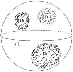
Figure 5.

(3.0.7) $$S_{1}=D_{1}/Q_{1},\cdots,S_{n}=D_{n}/Q_{n}\hskip 28.45274ptand\hskip 28.45274ptS_{n+1}=\Omega_{0}/G.$$

3.1. Fundamental domain of the group $G$

Let $K_{i}=F_{i}\cup F_{i}^{\prime}$ be a fundamental domain for the group $Q_{i}$ such that $F_{i}\subset D_{i}$ and $F_{i}^{\prime}\subset D_{i}^{\prime}$. Then a fundamental domain for the group $G$ is ( Figure 6 )

(3.1.1) $$K=(\bigcup_{i=1}^{n}F_{i})\cup(\bigcap_{i=1}^{n}F_{i}^{\prime}).$$

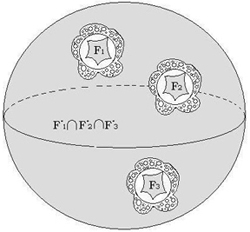
Figure 6.

In this case we have $p_{n+1}=p_{1}+p_{2}+\cdots+p_{n}.$

Now, lets consider the general case that there is a Schottky group $\Gamma_{0}=<\gamma_{01},...,\gamma_{0p_{0}}>$ (of order $p_{0}$) in the decomposition of the group $G$. Again we know that all other components of $\Omega(G)$ than $\Omega_{0}$ is simply connected. Then $\partial M_{\Gamma_{0}}$ can not be glued to the components other than $S_{n+1}$ in $\partial M_{G}$. Also this means that in this case we have

$$\Omega_{0}=(\mathbb{\hat{C}}\setminus(\bigcup_{i=1}^{n}\bigcup_{g\in G}g({\bar{D}}_{i})))\setminus\bigcup_{g\in G}g(\Lambda(\Gamma_{0}))=\bigcap_{g\in G}(\bigcap_{i=1}^{n}g(D_{i}^{\prime})\setminus g(\Lambda(\Gamma_{0})))$$

And

(3.1.2) $$\Lambda(G)=\bigcup_{i=1}^{n}\bigcup_{g\in G}g(\Lambda(Q_{i})\cup\Lambda(\Gamma_{0})).$$

In this case if $\{A_{1},...,A_{2p_{0}};\gamma_{01},...,\gamma_{0p_{0}}\}$ be a marking for the Schottky group $\Gamma_{0}$, then the fundamental domain is

(3.1.3) $$K=(\bigcup_{i=1}^{n}F_{i})\cup((\bigcap_{i=1}^{n}F_{i}^{\prime})\backslash\bigcup_{i=1}^{p_{0}}(A_{i}\cup\bar{A}_{p_{0}+i})).$$

And also for the genus of the component $S_{n+1}$ we have $p_{n+1}=p_{0}+p_{1}+\cdots+p_{n}$.

3.2. Green’s Function on $S_{i}$

For each $i=1,...,n$ lets consider

(3.2.1) $$Q_{i}=\langle\{q_{ij};j=1,...,2p_{i}\};\prod_{j=1}^{p_{i}}[q_{ij},q_{ip_{i}+j}]=I\rangle.$$

Then we can compute Green’s function on the components $S_{i}$ for $i=1,...,n$ as like as the previous section.

3.3. Schottky group associated to the group $G$

From the definition of $Q_{i}$ we know that $Q_{i}/N_{i}$ is a free group generated by $p_{i}$ generators. We have the following lemma

Lemma 3.3.1.

Lets denote by $N$ the smallest normal subgroup of the group $Q_{1}\ast\cdots\ast Q_{n}$ including the generators $q_{ij}$ for $i=1,...,n$ and $j=p_{i}+1,...,2p_{i}$ and $N_{i}$ be the smallest normal subgroup of the group $Q_{i}$ including the generators $q_{ij}$ for $j=p_{i}+1,...,2p_{i}$. Then we have

(3.3.1) $$\frac{Q_{1}\ast\cdots\ast Q_{n}}{N}\cong\frac{Q_{1}}{N_{1}}\ast\cdots\ast\frac{Q_{n}}{N_{n}}.$$

Proof.

In the case $n=2$ the map

$\varphi:Q_{1}\ast Q_{2}\longrightarrow\frac{Q_{1}}{N_{1}}\ast\frac{Q_{2}}{N_{2}}$

$x_{1}...x_{k}\longmapsto\bar{x}_{1}...\bar{x}_{k}$

is an isomorphism. The general case is true by induction on $n$. ∎

Now if $N$ be the smallest normal subgroup of the group $G$ including the generators $q_{ij}$ for $i=1,...,n$ and $j=p_{i}+1,...,2p_{i}$, Then by the previous lemma one can see that $G/N$ is isomorphic to the group

$$\Gamma_{0}\ast\frac{Q_{1}}{N_{1}}\ast\cdots\ast\frac{Q_{n}}{N_{n}}=\Gamma_{0}\ast\Gamma_{1}\ast\cdots\ast\Gamma_{n}.$$

Then $G/N$ is a free group of order $p_{n+1}$.

Now lets consider the covering space map $\Omega_{0}\longrightarrow S_{n+1}$. Since $N$ is a normal subgroup of $G$ then the covering space $\Omega_{0}/N\longrightarrow S_{n+1}$ is regular and is between $\Omega_{0}\longrightarrow S_{n+1}$ with the covering transformations group $Aut(\Omega_{0}/N)=G/N$ that is a free group of order $p_{n+1}$. Then similar to the previous section we have a Schottky group $\Gamma=\langle\gamma_{i1},\gamma_{i2},...,\gamma_{ip_{i}}\quad|\quad i=0,...,n\quad\rangle$ ( we can arrange the generators of the group $\Gamma$ in this way because of the isometry ) and a complex - analytic covering mapping $J:\Omega_{0}\longrightarrow\Omega(\Gamma)$ such that the following diagram is commutative

$\Omega_{0}\hskip 22.76219pt\overset{J}{\longrightarrow}\hskip 14.22636pt\Omega(\Gamma)$

$\pi_{G}\searrow\hskip 28.45274pt\swarrow\pi_{\Gamma}$

$S_{n+1}$

and for $i=1,...,n$ and $j\leq p_{i}$, $J\circ q_{ij}=\gamma_{ij}\circ J$ and for $j>p_{i}$, $J\circ q_{ij}=J$ and $J\circ\gamma_{0j}=\gamma_{0j}\circ J$ (we have considered the same notations for the generators of $\Gamma_{i}$ and $\Gamma$ ). As a matter of fact there is a Fuchsian group $F$ and there are normal subgroups $H_{1}$ and $H_{2}$ of $F$ such that the sequence

(3.3.2) $$H^{2}\overset{J^{\prime}}{\longrightarrow}\frac{H^{2}}{H_{1}}\cong\Omega_{0}\overset{J}{\longrightarrow}\frac{H^{2}}{H_{2}}\cong\frac{\Omega_{0}}{N}\longrightarrow S_{n+1}$$

is the composition of analytic covering maps. Then we have the composition of covering maps

(3.3.3) $$H^{2}\quad\overset{J\circ J^{\prime}}{\longrightarrow}\quad\frac{H^{2}}{H_{2}}\cong\frac{\Omega_{0}}{N}\quad\longrightarrow S_{n+1}$$

and since $F/H_{2}=Aut(\Omega_{0}/N)=G/N$ is a free group, like the previous section we have $\Omega_{0}/N\cong H^{2}/H_{2}\cong\Omega(\Gamma)$ for some Schottky group $\Gamma$. In fact, for the first, because of the isometries $F/H_{1}=Aut(H^{2}/H_{1}\cong\Omega_{0})=G$ we can choose the Fuchsian group

(3.3.4) $$F=\langle\{f_{ij}\ ;i=0,\ldots,n\quad j=1,...,2p_{i}\};\prod_{i=0}^{n}\prod_{j=1}^{p_{i}}[f_{ij},f_{i,p_{i}+j}]=I\quad\rangle$$

such that the equations $g_{ij}\circ J^{\prime}=J^{\prime}\circ f_{ij}$ for $i=1,...,n$ and $j=1,...,p_{i}$ are satisfied. Where $g_{ij}(=q_{ij}\quad or\quad\gamma_{0j})$ are the generators of $G$. Then like the previous section we can choose uniquely up to conjugation in $\mathrm{PGL}(2,\mathbb{C})$ the Schottky group $\Gamma$ that satisfies the equations

(3.3.5) $$(J\circ J^{\prime})\circ f_{ij}=\gamma_{ij}\circ(J\circ J^{\prime})\hskip 14.22636ptand\hskip 14.22636pt(J\circ J^{\prime})\circ f_{ip_{i}+j}=J\circ J^{\prime}$$

Then since $J^{\prime}$ is onto, the relations $J\circ g_{ij}=\gamma_{ij}\circ J$ and $J\circ g_{ip_{i}+j}=J$ are satisfied automatically for $i=1,...,n$ and $j=1,...,p_{i}$. This means that the following diagram is commutative in all loops

$$H^{2}\quad\overset{J^{\prime}}{\longrightarrow}\quad\Omega_{0}\quad\overset{J}{\longrightarrow}\quad\Omega(\Gamma)$$

$$\quad f_{ij}\updownarrow\hskip 36.98857ptg_{ij}\updownarrow\hskip 42.67912pt\gamma_{ij}\updownarrow\hskip 36.98857pt$$

$$H^{2}\quad\overset{J^{\prime}}{\longrightarrow}\quad\Omega_{0}\quad\overset{J}{\longrightarrow}\quad\Omega(\Gamma)$$

This gives a proof for the existing the of covering space $\Omega(\Gamma)$ and Schottky group $\Gamma$ satisfying the properties that we need and also shows the relations between the Fuchsian group $F$ , Kleinian group $G$ and the Schottky group $\Gamma$ associated to $S_{n+1}$.

Now lets put $G_{0}=\Gamma_{0}\ast Q_{10}\ast Q_{20}\ast\cdots\ast Q_{n0}$. Where $Q_{i0}$ is the free subgroup of $Q_{i}$ generated by the elements $q_{i1},...,q_{ip_{i}}$. For the extension of $J$ to $\Lambda(G_{0})$ i.e. defining the map $J:\Omega_{0}\cup\Lambda(G_{0})\longrightarrow\mathbb{\hat{C}}$, we know that each $Q_{i0}$ is free and purely loxodromic then it is a Schottky group. Like the previous section we can code an element of $\Lambda(Q_{i0})$ by Schottky coding $x=\cdots q_{ij_{2}}^{\epsilon_{j_{2}}}q_{ij_{1}}^{\epsilon_{j_{1}}}q_{ij_{0}}^{\epsilon_{j_{0}}}(x_{0})$ for $j_{k}\leq p_{i}$ and a point $x_{0}$ in $\Omega_{0}\subset D^{\prime}_{i}$. For each element $g$ in $G_{0}$ lets denote by $\gamma$ the element in $\Gamma$ corresponding to $g$, such that $J\circ g=\gamma\circ J$. Now put

$$J_{0}:\bigcup_{g\in G}g(\Lambda(\Gamma_{0}))\longrightarrow\Lambda(\Gamma)$$

$$g(\cdots\gamma_{i_{2}}^{\epsilon_{2}}\gamma_{i_{1}}^{\epsilon_{1}}\gamma_{i_{0}}^{\epsilon_{0}}(x_{0}))\mapsto\gamma(\cdots\gamma_{0i_{2}}^{\epsilon_{2}}\gamma_{0i_{1}}^{\epsilon_{1}}\gamma_{0i_{0}}^{\epsilon_{0}}(z_{0}))$$

Where $z_{0}=J(x_{0})$. And for $i=1,...,n$ put

$$J_{i}:\bigcup_{g\in G}g(\Lambda(Q_{i0}))\longrightarrow\Lambda(\Gamma)$$

$$g(\cdots q_{ij_{2}}^{\epsilon_{j_{2}}}q_{ij_{1}}^{\epsilon_{j_{1}}}q_{ij_{0}}^{\epsilon_{j_{0}}}(x_{0}))\mapsto\gamma(\cdots\gamma_{ij_{2}}^{\epsilon_{j_{2}}}\gamma_{ij_{1}}^{\epsilon_{j_{1}}}\gamma_{ij_{0}}^{\epsilon_{j_{0}}}(z_{0}))$$

And finally lets define

$$J:\Lambda(G_{0})\longrightarrow\Lambda(\Gamma)$$

$$J(x)=\begin{cases}J_{0}(x)&if~{}x\in\bigcup_{g\in G}g(\Lambda(\Gamma_{0}))\\ ~{}\\ J_{i}(x)&if~{}x\in\bigcup_{g\in G}g(\Lambda(Q_{i0}))\end{cases}.$$

Then like the previous section we can show that for each element $g$ in $G_{0}$ and $\gamma$ the element of $\Gamma$ corresponding to $g$ and each $x$ in $\Lambda(G_{0})$ we have $J\circ g(x)=\gamma\circ J(x)$ and $J(z^{\pm}(g))=z^{\pm}(\gamma)$. Also like the previous chapter we can consider the Fuchsian coding for the points of $\Lambda(G_{0})$ and from (2.5.1) we can explain $J$ and consequently the Green’s function on $S_{n+1}$ via the Fuchsian coding.

3.4. Green’s function of $S_{n+1}$

If we consider the condition $a(\Gamma)<1$ and use the subgroup $G_{0}=\Gamma_{0}\ast Q_{10}\ast Q_{20}\ast\cdots\ast Q_{n0}$ instead of $F_{0}$ in the previous section then one can bring all of the definitions like before with some changes, and compute the Green’s function on $S_{n+1}$ and the other parts in the same way. In this case we should notice that if $\{a_{ij},b_{ij}|i=0,...,n,j=1,...,p_{i}\}$ be a set that makes a base for $H_{1}(S_{n+1},\mathbb{Z})$ then each member of it has a class of images in $\Omega_{0}$. But we can consider that the representatives that are used in the computations are in the fundamental domain. As its shown in figure 6. In this case these images are in $D_{i}^{\prime}\cap\Omega_{0}$ for $i=1,...,n$ and also in $\Omega(\Gamma_{0})\cap\Omega_{0}$ for $i=0$. Then the representatives for $S_{i}$ and $S_{n+1}$ are coincide if we uniformize $S_{i}$ by $D^{\prime}_{i}$, i.e. identifying both components of $\partial M_{Q_{i}}$. Final formula for the Green’s function on $S_{n+1}$ is as following

$$g_{s_{n+1}}((a)-(b) ,(c)-(d))=\sum_{f\in G_{0}}\log\mid\langle J(a),J(b),J(f(c)),J(f(d))\rangle\mid$$

(3.4.1) $$-\sum_{\begin{subarray}{c}i=0,...,n\\ j=1,...,p_{i}\end{subarray}}\overline{X}_{ij}(a,b)\sum_{f\in S(f_{ij})}\log\mid\langle J(z^{+}(f)),J(z^{-}(f)),J(c),J(d)\rangle\mid$$

Where $f_{ij}$ is equal to $q_{ij}$ for $i=1,...,n$ and to $\gamma_{0j}$ for $i=0$, and $\overline{X}_{ij}(a,b)$ are the multipliers for $g_{s_{n+1}}$.

3.5. Remark (Infinitely many boundary component case )

When we have infinitely many boundary components in the boundary of $N_{G}$ that are Riemann surfaces without puncture, according to the Ahlfors finiteness theorem, $G$ is an infinitely generated Kleinian group. And hence one of the boundary components of $M_{G}$ is with infinity genus and is not a compact Riemann surface then for this component the Green’s function is not defined. But for the other components we can bring the computations similar to the previous condition using some subgroups of $G$ that are isomorphic to the Kleinian groups in the previous sections.

References

- [1] L. V. Ahlfors. ”Finitely Generated Kleinian Groups”. Amer.J. Math . 86 (1964),413-429 and 87(1965),759.
-
[2]
L. Bers. ”Uniformization, moduli and Kleinian groups” . Bull. London Math. Soc., 4(1972),257.300.
- [3] R. Bowen. ”Hausdorff dimension of quasi - circles” Publ. Math. IHES 50,11-25(1979).
- [4] R. Bowen. C. Series. ”Markov maps associated with fuchsian groups”. Publications mathématiques de l’I.H.E.S.,tome 50(1979),p.153-170.
- [5] G. Cornel, J.H. Silverman. ”Arithmetic Geometry”. Springer Verlag (1986).
- [6] G. Faltings. ” Calculating on arithmetic surfaces”. Ann. Math. 119, 387-424 (1982).
- [7] L. R. Ford. ”Automorphic Functions”. McGraw-Hill 1929.
- [8] D. Hejhal . ”On Schottky and Teichmuller spaces”. Ad. Math. 15, 133-156 (1975).
- [9] J. Jost. ”Compact Riemann Surfaces”. Springer.
- [10] P. Koebe. ”Uber die uniformisierung der algebraischen Kurven”. IV, Math. Ann. 75 (1914)
- [11] S. Lang. ”Introduction to Arakelov Theory” . New York Berlin Heidelberg: Springer 1988.
- [12] Yu. I. Manin. ”Three-dimensional hyperbolic geometry as - adic Arakelov geometry”. Invent. Math. 104 (1991), no. 2, 223–243.
- [13] Yu. I. Manin, V. Drinfeld, ”Periods of P - adic Schottky groups”. J. reine angew. Math. 262/263 (1973), 239–247.
- [14] Yu. I. Manin, Matilde Marcolli. ”Holographi Principle and Arithmetic curves”.
- [15] K. Matsuzaki, M. Taniguchi. ”Hyperbolic manifolds and Kleinian groups”. Oxford University Press, 1998.
- [16] C. McMullen. ”Riemann surfaces and the geometrization of 3 - manifolds”. Bull. Amer. Math. Soc. (N.S.) 27 (1992), no. 2, 207–216.
- [17] A. Marden. ”The Geometry of Finitely Generated Kleinian Groups”. The Annals of Mathematics, 2nd Ser. Vol. 99, No. 3 (May, 1974), pp. 383-462.
- [18] J. G. Ratcliffe. ”Foundations of Hyperbolic Manifolds” Springer Verlag (1991).
- [19] P. Zograf, L. Takhtajan. ”On the uniformization of Riemann surfaces and on the Weil-Petersson metric on the Teichmuller and Schottky spaces”. Math. USSR-Sb. 60 (1988), no.2, 297-313.