Deterministic Partial Differential Equation Model for Dose Calculation in Electron Radiotherapy

Abstract

Treatment with high energy ionizing radiation is one of the main methods in modern cancer therapy that is in clinical use. During the last decades, two main approaches to dose calculation were used, Monte Carlo simulations and semi-empirical models based on Fermi-Eyges theory. A third way to dose calculation has only recently attracted attention in the medical physics community. This approach is based on the deterministic kinetic equations of radiative transfer. Starting from these, we derive a macroscopic partial differential equation model for electron transport in tissue. This model involves an angular closure in the phase space. It is exact for the free-streaming and the isotropic regime. We solve it numerically by a newly developed HLLC scheme based on [8], that exactly preserves key properties of the analytical solution on the discrete level. Several numerical results for test cases from the medical physics literature are presented.

1 Introduction

Mathematical methods play an increasing role in medicine, especially in radiation therapy. Several special journal issues have been devoted to cancer modeling and treatment, cf. [4, 5, 6, 12] among others.

Together with surgery and chemotherapy, the use of ionizing radiation is one of the main tools in the therapy of cancer. The aim of radiation treatment is to deposit enough energy in cancer cells so that they are destroyed. On the other hand, healthy tissue around the cancer cells should be harmed as little as possible. Furthermore, some regions at risk, like the spinal chord, should receive a dose below a certain threshold.

Most dose calculation algorithms in clinical use rely on the Fermi–Eyges theory of radiation which is insufficient at inhomogenities, e.g. the lung. This work, on the other hand, starts with a Boltzmann transport model for the radiation which accurately describes all physical interactions.

Until recently, dose calculation using a Boltzmann transport equation has not attracted much attention in the medical physics community. This access is based on deterministic transport equations of radiative transfer. Similar to Monte Carlo simulations it relies on a rigorous model of the physical interactions in human tissue that can in principle be solved exactly. Monte Carlo simulations are widely used, but it has been argued that a grid-based Boltzmann solution should have the same computational complexity [9]. Electron and combined photon and electron radiation were studied in the context of inverse therapy planning, cf. [35, 34] and most recently [36]. A consistent model of combined photon and electron radiation was developed [22] that includes the most important physical interactions. Furthermore, several neutral particle codes have been applied to the dose calculation problem, see [19] for a review and most recently [38].

In this paper, we want to study a macroscopic approximation to the mesoscopic transport equation. After the problem formulation in section 2, we derive the approximation of the macroscopic model in section 3. This approximation consists of a system of nonlinear hyperbolic partial differential equations, whose properties we briefly discuss. Due to the possibility of shock solutions, hyperbolic PDEs have to be solved with great care. In section 5, we introduce a scheme which is adapted to the problem at hand. Numerical results for tests from the medical physics literature are presented in section 6.

2 A deterministic model for dose calculation

A ray of high energy electrons that interacts with human tissue is subject to elastic scattering processes and inelastic ones. It is this latter process that leads to energy deposition in the tissue i.e. to absorbed dose.

To formulate a transport equation for electrons we study their fluence in phase space. Let $\psi(r,\epsilon,\Omega)\cos\Theta dAd\Omega d\epsilon dt$ be the number of electrons at position $r$ -$r$ being a vector in 2D or 3D space- that move in time $dt$ through area $dA$ into the element of solid angle $d\Omega$ around $\Omega$ with an energy in the interval $(\epsilon,\epsilon+d\epsilon)$. The angle between direction ${\Omega}$ and the outer normal of $dA$ is denoted by $\Theta$. The kinetic energy $\epsilon$ of the electrons is measured in units of $m_{e}c^{2}$, where $m_{e}$ is the electron mass and c is the speed of light.

2.1 Boltzmann transport equation

The transport equation can generally be formulated as [14]

$${\Omega}\cdot\nabla\psi(r,\epsilon,\Omega) = \rho_{\rm in}({r})\int\limits_{\epsilon}^{\infty}\int\limits_{{\mathcal{S}}^{2}}{\sigma}_{\rm in}(\epsilon^{\prime},\epsilon,{\Omega}^{\prime}\cdot{\Omega})\psi(r,\epsilon^{\prime},\Omega^{\prime})d\Omega^{\prime}d\epsilon^{\prime}$$ (1)

$$+ \rho_{\rm el}({r})\int\limits_{{\mathcal{S}}^{2}}\sigma_{\rm el}({r},\epsilon,{\Omega}^{\prime}\cdot{\Omega})\psi(r,\epsilon,\Omega^{\prime})d\Omega^{\prime}$$

$$- \rho_{\rm in}({r})\sigma_{\rm in}^{\rm tot}(\epsilon)\psi(r,\epsilon,\Omega)$$

$$- \rho_{\rm el}({r})\sigma_{\rm el}^{\rm tot}({r},\epsilon)\psi(r,\epsilon,\Omega),$$

with ${\sigma}_{\rm in}$ being the differential scattering cross section for inelastic scattering, and $\sigma_{\rm el}$ the differential cross section for elastic scattering; $\sigma_{\rm in}^{\rm tot}=\int_{S^{2}}{\sigma}_{\rm in}d\Omega$ and $\sigma_{\rm el}^{\rm tot}=\int_{S^{2}}{\sigma}_{\rm el}d\Omega$ are the total cross sections for inelastic and elastic scattering, respectively; $\rho_{\rm in}$ and $\rho_{\rm el}$ are the densities of the respective scattering centers.

Explicit formulas for the cross sections that we used in this model can be found in section 2.3. They are based on the model developed in [22]. The energy integration is performed over $(\epsilon,\infty)$ since the electrons lose energy in every scattering event. Also, we consider only electron radiation. Equation (1) could also be used to model electrons which are generated by the interactions of photons with matter, as in [22]. In this case we would have an additional source term on the right hand side for the generated electrons.

Besides the transport equation one needs an equation for the absorbed dose. It was derived in [22] as an asymptotic limit of a model with a finite lower energy bound $\epsilon_{\rm s}>0$. The formula is exact if one chooses the lower energy limit $\epsilon_{\rm s}=0$, as we do here.

$$D({r})=\frac{T}{\rho({r})}\int_{0}^{\infty}S({r},\epsilon^{\prime})\psi^{(0)}({r},\epsilon^{\prime})d\epsilon^{\prime}$$ (2)

with

$$\psi^{(0)}({r},\epsilon):=\int\limits_{S^{2}}\psi({r},\epsilon,{\Omega}^{\prime})d\Omega^{\prime},$$

$T$ being the duration of the irradiation of the patient and $\rho$ the mass density of the irradiated tissue. If all quantities are calculated in SI units, equation (2) leads to SI units J/kg or Gray (Gy) for the dose.

$S$ is the stopping power related to the inelastic cross section. It is defined as

$$S({r},\epsilon)=\rho_{\rm in}({r})\int\limits_{0}^{\epsilon}\epsilon^{\prime}\sigma_{\rm in}(\epsilon,\epsilon^{\prime})d\epsilon^{\prime}.$$

2.2 Continuous slowing-down approximation

Electron transport in tissue has very distinctive properties. The soft collision differential scattering cross sections have a pronounced maximum for small scattering angles and small energy loss. This allows for a simplification of the scattering terms in the Boltzmann equation. The Fokker-Planck equation is the result of an asymptotic analysis for both small energy loss and small deflections. It has been rigorously derived in [31] and has been applied to the above Boltzmann model in [22]. However, some electrons will also experience hard collisions with large changes in direction and energy losses which have to be described by Boltzmann integral terms. Thus we only use an asymptotic analysis to describe energy loss, called continuous slowing-down approximation. This approximation has a greater domain of validity than the Fokker-Planck approximation. The Boltzmann equation in continuous slowing-down approximation (BCSD) is [25]

$${\Omega}\cdot\nabla\psi(r,\epsilon,\Omega) = \rho_{\rm in}({r})\int\limits_{{\mathcal{S}}^{2}}{\sigma}_{\rm in}^{\rm CSD}(\epsilon,{\Omega}^{\prime}\cdot{\Omega})\psi(r,\epsilon,\Omega^{\prime})d\Omega^{\prime}$$ (3)

$$+ \rho_{\rm el}({r})\int\limits_{{\mathcal{S}}^{2}}\sigma_{\rm el}({r},\epsilon,{\Omega}^{\prime}\cdot{\Omega})\psi(r,\epsilon,\Omega^{\prime})d\Omega^{\prime}$$

$$- \rho_{\rm in}({r})\sigma_{\rm in,\rm tot}(\epsilon)\psi(r,\epsilon,\Omega)$$

$$- \rho_{\rm el}({r})\sigma_{\rm el,\rm tot}({r},\epsilon)\psi(r,\epsilon,\Omega)$$

$$+ \frac{\partial}{\partial\epsilon}(S(r,\epsilon)\psi(r,\epsilon,\Omega))$$

with

$${\sigma}_{\rm in}^{\rm CSD}=\int_{0}^{\infty}\sigma_{\rm in}(\epsilon,\epsilon^{\prime},\mu)d\epsilon^{\prime}.$$

A truncation in the energy space is introduced, that does not allow particles with arbitrary high energy,

$$\lim_{\epsilon\to\infty}\psi(r,\epsilon,\Omega)=0.$$ (4)

In the numerical simulations, we use a sufficiently large cutoff energy. Furthermore, we prescribe the ingoing radiation at the spatial boundary,

$$\psi(r,\epsilon,\Omega)=\psi_{b}(r,\epsilon,\Omega)\quad\textrm{for}\quad n\cdot\Omega<0,$$ (5)

where $n$ is the unit outward normal vector.

2.3 Modeling of Scattering Cross Sections

2.3.1 Henyey-Greenstein Scattering Theory

The detailed interactions of electrons with atoms give rise to complicated explicit formulas for the scattering coefficients. Because of this, many studies use the simplified Henyey-Greenstein scattering kernel for elastic scattering [2],

$$\sigma_{HG,g}(\mu)=\frac{1-g^{2}}{4\pi(1+g^{2}-2g\mu)^{3/2}}.$$ (6)

The parameter $g$, which can depend on $r$, is the average cosine of the scattering angle and is a measure for the anisotropy of the scattering. The case where $g\leq 1$ matches an anisotropic scattering configuration.

2.3.2 Mott and Møller Scattering

A more realistic model for elastic and inelastic scattering of electrons in tissue has been developed in [22]. This model introduces material parameters (namely densities $\rho_{e}$ and $\rho_{c}$, ionization energy $\epsilon_{B}$ and effective atomic charge $Z$). The energy integration for inelastic scattering is cut-off at $\epsilon_{B}$.

The model uses the Mott scattering formula for elastic scattering of an electron by an ion [29, 26]

$$\sigma_{\rm Mott}({r},\epsilon,{\Omega}^{\prime}\cdot{\Omega})=\frac{Z^{2}({r})r_{\rm e}^{2}(1+\epsilon)^{2}}{4[\epsilon(\epsilon+2)]^{2}(1+2\eta({r},\epsilon)-\cos\vartheta)^{2}}\left[1-\frac{\epsilon(\epsilon+2)}{(1+\epsilon)^{2}}\sin^{2}\frac{\vartheta}{2}\right],$$

with $\vartheta=\arccos({\Omega}^{\prime}\cdot{\Omega})$, and $\epsilon$ is the outcoming electron energy in $m_{e}c^{2}$ units. Here, $\alpha\approx 1/137$ is the fine structure constant, $Z$ is the atomic number of the irradiated medium, $r_{\rm e}$ is the classical electron radius. $Z$ depends on ${r}$ to account for heterogeneous media. To avoid an otherwise occurring singularity at $\vartheta=0$ a screening parameter

$$\eta(r,\epsilon)=\frac{\pi^{2}\alpha^{2}Z^{2/3}(r)}{\epsilon(\epsilon+2)},$$

can be introduced [39] that models the screening effect of the electrons of the atomic shell, denoted by $a$.

The inelastic scattering process is Møller scattering, where an electron impinges an atom that releases itself an additional electron

$$e^{-}+a\rightarrow a^{+}+2\ e^{-}$$

For this process, the electrons can be considered indistinguishable. The electron which has the higher energy after the collision is called primary electron, the other electron secondary. Due to kinematical reasons of the scattering processes the range of solid angles in Møller scattering is restricted. After the collision, the angle between the directions of the electrons is at most $\pi/2$. For an angle in $[0,\pi/4]$, the electron with energy $\epsilon$ is the primary electron, for an angle in $[\pi/4,\pi/2]$, it is the secondary electron. Therefore the Møller cross section can be written as

$$\sigma_{M}=\tilde{\sigma}_{M}\chi_{\{0<\Omega\cdot\Omega^{\prime}<\sqrt{2}/2\}}+\tilde{\sigma}_{M,\delta}\chi_{\{\sqrt{2}/2<\Omega\cdot\Omega^{\prime}<1\}},$$

where $\chi$ denotes the characteristic function of a set,

$$\tilde{\sigma}_{\rm M}(\epsilon^{\prime},\epsilon,{\Omega}^{\prime}\cdot{\Omega})=\sigma_{\rm M}(\epsilon^{\prime},\epsilon)\delta_{M}(\mu,\mu_{p})\frac{1}{2\pi},\quad\mu={\Omega}^{\prime}\cdot{\Omega},$$

is the Møller differential cross section of primary electrons and

$$\tilde{\sigma}_{\rm M,\delta}(\epsilon^{\prime},\epsilon,{\Omega}^{\prime}\cdot{\Omega})=\sigma_{\rm M}(\epsilon^{\prime},\epsilon)\delta_{\rm M,\delta}(\mu,\mu_{\delta})\frac{1}{2\pi},\quad\mu={\Omega}^{\prime}\cdot{\Omega},$$

is the Møller differential cross section of secondary electrons. Here,

$$\sigma_{\rm M}(\epsilon^{\prime},\epsilon)=\frac{2\pi r_{\rm e}^{2}(\epsilon^{\prime}+1)^{2}}{\epsilon^{\prime}(\epsilon^{\prime}+2)}\left[\frac{1}{\epsilon^{2}}+\frac{1}{(\epsilon^{\prime}-\epsilon)^{2}}+\frac{1}{(\epsilon^{\prime}+1)^{2}}-\frac{2\epsilon^{\prime}+1}{(\epsilon^{\prime}+1)^{2}\epsilon(\epsilon^{\prime}-\epsilon)}\right],$$

and

$$\delta_{M}(\mu_{\rm e},\mu_{p}) =\delta\left(\mu_{\rm e}-\sqrt{\frac{\epsilon}{\epsilon^{\prime}}\frac{\epsilon^{\prime}+2}{\epsilon+2}}\right),\text{ for }\epsilon>\frac{(\epsilon^{\prime}-\epsilon_{\rm B})}{2},$$

$$\delta_{\rm M,\delta}(\mu_{\rm e},\mu_{\delta}) =\delta\left(\mu_{\rm e}-\sqrt{\frac{\epsilon}{\epsilon^{\prime}}\frac{\epsilon^{\prime}+2}{\epsilon+2}}\right),\quad\epsilon<\frac{(\epsilon^{\prime}-\epsilon_{\rm B})}{2}.$$

In the simulations the model parameters $\rho_{\rm el}$, $\rho_{\rm in}$, $\epsilon_{B}$ and $Z$ are fitted to tabulated values taken from the database of the PENELOPE Monte Carlo code [32].

3 Partial Differential Equation Model

We will try to reduce the cost of solving system (1) by assuming a minimum entropy principle for the angle distribution of particles. This principle has been first proposed by Jaynes [24] as a method to select the most likely state of a thermodynamical system having only incomplete information. It has subsequently been developed in [28], [27], [1] and [15], among others, and has become the main concept of rational extended thermodynamics [30]. A full account and an exhaustive list of references on the historical development can be found in [21].

We define the first three moments in angle:

$$\psi^{(0)}(r,\epsilon) =\int_{S^{2}}\psi(r,\epsilon,\Omega)d\Omega,$$ (7)

$$\psi^{(1)}(r,\epsilon) =\int_{S^{2}}\Omega\psi(r,\epsilon,\Omega)d\Omega,$$ (8)

$$\psi^{(2)}(r,\epsilon) =\int_{S^{2}}(\Omega\otimes\Omega)\psi(r,\epsilon,\Omega)d\Omega,$$ (9)

where we note that $\psi^{(0)}$ is a scalar, $\psi^{(1)}$ is a vector and $\psi^{(2)}$ is a tensor.

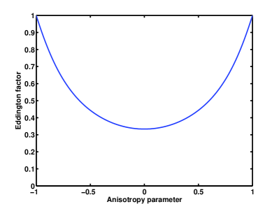
(a) Eddington factor.

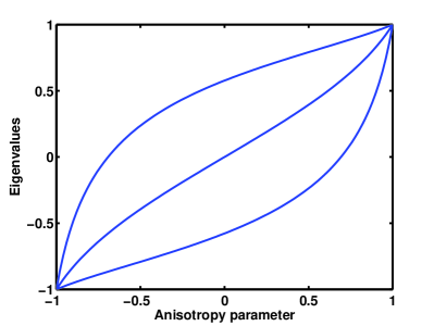
(b) Eigenvalues.

Figure 1: Eddington factor $\chi$ and system eigenvalues versus anisotropy parameter $|\alpha|$.

If we integrate the system (3) over $\Omega$, we can derive the following equations,

$$\nabla_{x}\psi^{(1)} =\frac{\partial}{\partial\epsilon}(S\psi^{(0)}),$$ (10a)

$$\nabla_{x}\psi^{(2)} =-(T_{M}+T_{\rm Mott})\psi^{(1)}+\frac{\partial}{\partial\epsilon}(S\psi^{(1)}).$$ (10b)

We have introduced the transport coefficients

$$T_{\rm in}(r,\epsilon) =\pi\rho_{\rm in}(r)\int_{\epsilon_{B}}^{(\epsilon-\epsilon_{B})/2}\int_{-1}^{1}(1-\mu)\sigma_{\rm in}(\epsilon,\epsilon^{\prime},\mu)d\mu d\epsilon^{\prime},$$ (11)

$$T_{\rm{el}}(r,\epsilon) =\pi\rho_{\rm el}(r)\int_{-1}^{1}(1-\mu)\sigma_{\rm el}(\epsilon,\mu)d\mu.$$ (12)

These coefficients and the stopping power can be computed for both Henyey-Greenstein and Mott/Møller scattering. Explicit expressions can be found in [22, 17].

The remaining problem is the computation of moment $\psi^{(2)}$ as a function of $\psi^{(0)}$ and $\psi^{(1)}$. The Minimum Entropy $M_{1}$ closure for electrons [10] can be derived in the following way. To close the system we determine a distribution function $\psi_{ME}$ that minimizes the entropy of the electrons,

$$H_{R}^{\ast}(\psi)=-\int_{S^{2}}\psi\log\psi d\Omega,$$ (13)

under the constraint that it reproduces the lower order moments,

$$\int_{S^{2}}\psi_{ME}d\Omega=\psi^{(0)}\quad\textrm{and}\quad\int_{S^{2}}\Omega\psi_{ME}d\Omega=\psi^{(1)}.$$ (14)

By using this entropy, we have implicitly assumed that the electrons obey classical Maxwell-Boltzmann statistics. This is justified, since here quantum effects can be neglected.

Analogous to the calculations in [27] we can show that the entropy minimizer has the following form,

$$\psi_{ME}=a_{0}\exp(-\Omega\cdot a_{1}),$$ (15)

where $a_{0}$ is a non-negative scalar, and $a_{1}$ is a three component real valued vector. This is a Maxwell-Boltzmann type distribution and $a_{0}$, $a_{1}$ are (scaled) Lagrange multipliers enforcing the constraints. An important parameter is the anisotropy parameter $\alpha$,

$$\alpha=\frac{\psi^{(1)}}{\psi^{(0)}},$$

whose norm is by construction less than or equal to one. If we compute the different moments of the distribution function given by (15) we obtain,

$$\psi^{(0)}=4\pi a_{0}\frac{\sinh(|a_{1}|)}{|a_{1}|},\ \psi^{(1)}=4\pi a_{0}\frac{\sinh(|a_{1}|)(1-|a_{1}|\coth(|a_{1}|))}{|a_{1}|^{3}}\ a_{1}.$$ (16)

In fact, these relations can be combined to give,

$$\alpha=\frac{1-|a_{1}|\coth(|a_{1}|)}{|a_{1}|^{2}}\ a_{1},$$ (17)

or by taking the modulus,

$$|\alpha|=\frac{|a_{1}|\coth(|a_{1}|)-1}{|a_{1}|}.$$ (18)

The relation (18) cannot be inverted explicitly by hand, i.e. we cannot express $|a_{1}|$ as a function of $\alpha$ in a closed form. However, this relation determines a unique solution which can in principle be computed. If we assume that we know $a_{1}$, $\psi^{(2)}$ can be computed as

$$\psi^{(2)}=\psi^{(0)}\left(\frac{1-\chi(\alpha)}{2}I+\frac{3\chi(\alpha)-1}{2}\alpha\otimes\alpha\right),$$ (19)

where

$$\chi=\frac{|a_{1}|^{2}-2|a_{1}|\coth(|a_{1}|)+2}{|a_{1}|^{2}}$$ (20)

is a function of $\alpha$ by means of (18).

For its efficient numerical evaluation, the Eddington factor has to be approximated. Several possibilities exist:

• One could solve the closure relation (18) for $|a_{1}|$ e.g. by a Newton iteration in each step during the simulation.

• One could precompute a table that gives the Eddington factor $\chi$ as a function of $\alpha$.

• One could approximate $\chi(\alpha)$ by a suitable special function.

The second approach has been followed in [17]. It is advantageous only if the space in which one interpolates is low-dimensional. For more moments, this approach becomes more expensive, and the first approach appears to be more advantageous.

In some cases, an ansatz for $\chi$ can provide a good approximation. This is the approach we are following here. The Eddington factor $\chi$ can be approximated by a very simple rational function,

$$\chi(\alpha)\approx{\frac{a_{6}\,{\alpha}^{6}+a_{4}\,{\alpha}^{4}+a_{2}\,{\alpha}^{2}+a_{0}}{{\alpha}^{4}+b_{2}\,{\alpha}^{2}+b_{0}.}}$$ (21)

This approximation is very accurate (the difference with exact curve is about $10^{-15}$). The coefficients are given by

$$\begin{array}[]{cc}a_{0}=\ \ 0.762066949972264,&b_{0}=\ \ 2.28620084991677,\\ a_{2}=\ \ 0.219172080193380,&b_{2}=-2.10758208969840,\\ a_{4}=-0.259725400168378,&\\ a_{6}=\ \ 0.457105130221120.\end{array}$$ (22)

4 Properties of the System

In the literature, the system that has been thoroughly investigated (both analytically and numerically) is system (10) restricted to its conservative terms, without external sources, but with time-dependence.

In the present work, we adapt a pseudo-time technique. We focus on the spatial discretization and use a standard discretization for the terms on the right-hand side. Thus we consider

$$\frac{\partial}{\partial t}\psi^{(0)}+\nabla_{x}\psi^{(1)} =0,$$ (23a)

$$\frac{\partial}{\partial t}\psi^{(1)}+\nabla_{x}\psi^{(2)}\left(\psi^{(0)},\psi^{(1)}\right) =0,$$ (23b)

with the closure (18).

The Eddington factor $\chi$ is shown in Figure 1. Furthermore, we show the system eigenvalues in two dimensions. In the isotropic regime (anisotropy parameter zero), they coincide with the P1 eigenvalues. On the other hand, in the case of free-streaming ($|\alpha|=1$), they coincide and have absolute value one. Thus the system (10) is hyperbolic and the speed of propagation is limited by one. Moreover the system is hyperbolic symmetrisable [15].

System (23) closed by the relation (19) has been analyzed thoroughly in [23]. There, solutions to Riemann problems are constructed and invariant regions are computed. Since the reconstruction (15) of the kinetic distribution $\psi$ is always positive, it can be expected that system (19) - (23) must admit a positive solution $\psi^{(0)}$ and a limited flux $\|\alpha\|<1$. To our knowledge, however, there exists no proof of this fact. The invariant regions computed in [23] only cover a subset of all admissible values. For a related model [18], bounds were proved, but only in 1D and steady state. Nevertheless, we construct a scheme which preserves exactly the positivity of $\psi^{(0)}$ and the flux limitation, i.e. the convex set of the admissible states of the system (23) is [8]

$$\mathcal{A}=\left\{\left(\psi^{(0)},\psi^{(1)}\right):\ \psi^{(0)}\geq 0,\ |\psi^{(1)}|\leq\psi^{(0)}\right\}.$$

In the absence of sources or boundaries, the total mass, momentum and energy are conserved.

In addition, the minimum entropy system recovers the equilibrium diffusion regime as a relaxation limit for large absorption coefficients [13].

In a two- or three-dimensional geometry, we have in addition [8]: Let $n$ be the unit normal vector to an interface; then the system exhibits two acoustic waves, with velocities $\lambda_{L}(n)$ and $\lambda_{R}(n)$, supplemented by a contact wave with velocity $\beta(n)$. The quantity $\beta\cdot n$ satisfies the following inequality $\lambda_{L}(n)\leq\beta(n)\cdot n\leq\lambda_{R}(n)$. The Riemann invariants associated with the contact wave are $\left\{\beta,\Pi\right\}$. They are defined by the relations

$$\psi_{1} =\left(\Pi+\psi_{0}\right)\beta,$$ (24a)

$$\psi_{2} =\left(\psi_{0}+\Pi\right)\beta\otimes\beta+\Pi Id\ .$$ (24b)

5 Numerical Method

The properties of the continuous model should be reproduced by the numerical scheme. In particular the positivity and flux limitation constraints are fundamental. An HLL scheme [20] can be constructed [3, 11, 8], that satisfies the required properties. However such an approach cannot capture the contact discontinuity. To prevent this failure, an HLLC scheme [3] has been derived, that resolves the contact discontinuity and satisfies the physical constraints.

To complete this presentation of the numerical approximation, we mention that a suitable high order extension that preserves both the positivity and the flux limitation can be derived, relying on an appropriate limitation procedure.

5.1 An HLL scheme for the free transport $M_{1}$ angular moment system

In this section, we derive a Finite Volume method, issued from the HLL method [20] to discretize the free transport equation (23). Put in other words, we omit the source terms and we consider the one dimensional generic conservative system

$$\displaystyle\frac{\partial}{\partial t}\mathcal{U}+\frac{\partial}{\partial x}\left[\mathcal{F}\left(\mathcal{U}\right)\right]=0\ ,$$ (25)

where

$$\mathcal{U}=\left(\begin{array}[]{cc}\psi_{0}\\ \psi_{1}\end{array}\right)$$

and $\mathcal{F}$ stands for the flux of the $M_{1}$ system in the $x$ space direction.
We consider a structured mesh of size $\Delta x_{i}$, defined by the cells $I_{i}=\left[x_{i-1/2},x_{i+1/2}\right)$, where we have set $x_{i+1/2}=x_{i}+\Delta x/2\ ,i\in\mathbb{Z}$, at time $t^{n}$. As usual, we consider known a piecewise contant approximation $U^{h}(x,t^{n})$, defined by $U^{h}(x,t^{n})=U_{i}^{n},x\in I_{i}\ ,\forall i\in\mathbb{Z}$.

At initial time $t=0$, we impose

$$U_{i}^{0}=\displaystyle\int_{x_{i-1/2}}^{x_{i+1/2}}U_{0}(x)dx,$$

where $U_{0}$ is the initial data. This approximation evolves in time, involving a suitable approximate Riemann solver. In the HLL approach, the exact Riemann solver solution is substituted by a single approximate state (see Figure 2).

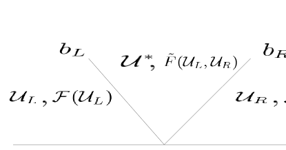
Figure 2: Structure of the approximate HLL Riemann Solver

Here $b_{L}$ and $b_{R}$ are relevant approximations of $\lambda_{L}$ and $\lambda_{R}$, respectively. Let us introduce the proposed approximate solution:

$${\mathcal{U}_{HLL}}(x,t)\equiv\left(\begin{array}[]{cc}\psi_{0}(x,t)\\ \psi_{1}(x,t)\end{array}\right)_{HLL}=\left\{\begin{array}[]{ccc}&{\mathcal{U}_{L}}&\ \mbox{if}\ \frac{x}{t}<b_{L}\ ,\\ &{\mathcal{U}^{*}}&\qquad\ \ \mbox{if}\ b_{L}\leq\frac{x}{t}\leq b_{R}\ ,\\ &{\mathcal{U}_{R}}&\ \mbox{if}\ b_{R}<\frac{x}{t}\ .\end{array}\right.$$ (31)

Moreover, the search of weak solutions leads to the Rankine-Hugoniot jump conditions

$$-b_{L}\left[\mathcal{U}^{*}-\mathcal{U}_{L}\right]+\left[\tilde{F}-\mathcal{F}(\mathcal{U}_{L})\right] =0,$$ (32a)

$$-b_{R}\left[\mathcal{U}_{R}-\mathcal{U}^{*}\right]+\left[\mathcal{F}(\mathcal{U}_{R})-\tilde{F}\right] =0.$$ (32b)

These relations provide us with an explicit expression for the intermediate state and flux of the numerical scheme

$$\mathcal{U}^{*} = \frac{b_{R}\mathcal{U}_{R}-b_{L}\mathcal{U}_{L}-(\mathcal{F}(\mathcal{U}_{R})-\mathcal{F}(\mathcal{U}_{L}))}{b_{R}-b_{L}}\ ,$$ (33a)

$$\tilde{F}(\mathcal{U}_{L},\mathcal{U}_{R}) = \frac{b_{R}\mathcal{F}(\mathcal{U}_{L})-b_{L}\mathcal{F}(\mathcal{U}_{R})-b_{L}b_{R}(\mathcal{U}_{R}-\mathcal{U}_{L})}{b_{R}-b_{L}}\ ,$$ (33b)

At each interface $x_{i+1/2}$, we impose the above HLL approximate Riemann solver, assuming the CFL like condition (34) ensuring that the Riemann solvers do not interact in the case where $b_{L,i+1/2}<0$ and $b_{R,i-1/2}>0$ :

$$\frac{\Delta t}{\Delta x}\leq\frac{b_{L,i+1/2}b_{R,i-1/2}}{b_{L,i+1/2}-b_{R,i-1/2}}\ .$$ (34)

We set $\mathcal{U}^{h}(x,t+\Delta t)$, at time $t^{n}+\Delta t$, the superposition of the non-interacting Riemann solutions. We define the updated approximation at time $t^{n+1}$ by

$$\mathcal{U}_{i}^{n+1}=\frac{1}{\Delta x}\int_{x_{i-1/2}}^{x_{i+1/2}}\mathcal{U}^{h}(x,t^{n}+\Delta t).$$

An easy computation gives

$$\mathcal{U}_{i}^{n+1}=\mathcal{U}_{i}^{n}-\frac{\Delta t}{\Delta x}({F}_{i+1/2}^{n}-{F}_{i-1/2}^{n})\ ,$$ (35)

where

$${F}_{i+1/2}^{n}(\mathcal{U}_{i}^{n},\mathcal{U}_{i+1}^{n})=\left\{\begin{array}[]{ccc}&\mathcal{F}\left(\mathcal{U}_{i}^{n}\right)&\ \mbox{if}\ 0<b_{L,i+1/2}\\ &\tilde{F}_{i+1/2}\left(\mathcal{U}_{i}^{n},\mathcal{U}_{i+1}^{n}\right)&\qquad\qquad\ \ \mbox{if}\ b_{L,i+1/2}\leq 0\leq b_{R,i+1/2}\\ &\mathcal{F}\left(\mathcal{U}_{i+1}^{n}\right)&\ \mbox{if}\ b_{R,i+1/2}<0\end{array}\right.$$

The robustness of the scheme, namely the positivity, the flux limitation, the total mass preservation, has been established for the HLL scheme (see [8] for further details).
Finally, concerning the high order extension, we adopt a van Leer MUSCL technique [37], supplemented by a suitable slope limitation preserving these expected physical properties [7].

5.2 An accurate HLLC scheme

The HLL scheme has proved to be robust, however, its 2D extension fails when approximating contact waves. Several works [3, 8] introduce a more accurate scheme, the HLLC scheme, based on a two state approximation, denoted by $U_{L}^{*}$ and $U_{R}^{*}$.

First, let us recall the relevant linearization that permits us to define an approximation with two intermediate states: on the one hand, the Rankine-Hugoniot conditions (32) are considered; on the other hand, they are supplemented by the continuity of the Riemann invariants accross the contact wave:

$$\left(\beta_{x}\right)_{L}^{*}=\left(\beta_{x}\right)_{R}^{*}=\beta_{x}^{*}\quad,\quad\Pi_{L}^{*}=\Pi_{R}^{*}=\Pi^{*}\ \ ,$$ (36)

where $\beta_{x}$ and $\Pi$ are defined by the relation (24). The combination of both the Rankine-Hugoniot condition (32) and the relation (36) standing as the continuity of the Riemann invariants accross the contact wave, is sufficient to determine uniquely [3, 8] the two approximate states $U_{L}^{*}$ and $U_{R}^{*}$, together with their associated fluxes $\tilde{F}_{L}$ and $\tilde{F}_{R}$. The proposed HLLC approximate solution can be written as

$${\mathcal{U}_{HLLC}}(x,t)\equiv\left(\begin{array}[]{cc}\psi_{0}(x,t)\\ \psi_{1}(x,t)\end{array}\right)_{HLLC}=\left\{\begin{array}[]{ccc}&{\mathcal{U}_{L}}&\ \mbox{if}\ \frac{x}{t}<b_{L}\ ,\\ &{\mathcal{U}^{*}_{L}}&\qquad\ \ \mbox{if}\ b_{L}\leq\frac{x}{t}\leq\beta_{x}^{*}\ ,\\ &{\mathcal{U}^{*}_{R}}&\qquad\ \ \mbox{if}\ \beta_{x}^{*}\leq\frac{x}{t}\leq b_{R}\ ,\\ &{\mathcal{U}_{R}}&\ \mbox{if}\ b_{R}<\frac{x}{t}\ .\end{array}\right.$$ (43)

Similar to the derivation of the HLL scheme, we integrate over a cell $I_{i}$ the juxtaposition of the non-interacting HLLC Riemann approximate solvers at each interface (projection step), in order to obtain the updated quantity

$$\mathcal{U}_{i}^{n+1}=\frac{1}{\Delta x}\int_{x_{i-1/2}}^{x_{i+1/2}}\mathcal{U}^{h}(x,t^{n}+\Delta t).$$

This brief description of the HLLC scheme is now completed. It is able to capture exactly the contact wave, and satisfies the positivity, the flux limitation, and the total mass preservation.

6 Numerical Results

6.1 Central Void

The first test case is taken from the medical physics literature [2]. We consider only elastic scattering, which is modeled by the Henyey-Greenstein kernel. Thus $S=0$ and $T_{\rm in}=0$. We compare the particle flux $\psi^{(0)}(x)$ obtained with the minimum entropy model (labeled M1) with a discrete ordinates solution of the transport equation (labeled SN) with sufficiently many angles (128). The method has been described in [16].

The test case consists of a one-dimensional geometry with three layers: optically thick, followed by optically thin followed again by optically thick. The layers have an equal depth of 40 mm. The scattering and absorption coefficients are $\sigma_{s}=0.5$ mm^-1, $\sigma_{a}=0.005$ mm^-1 for the optically thick region, and $\sigma_{s}=0.01$ mm^-1, $\sigma_{a}=0.0001$ mm^-1 for the optically thin region. Moreover, $g=0$. Figure 3 shows the particle flux $\psi^{(0)}$ as a functon of space. Compared to the benchmark solution, the minimum entropy model slightly overestimates but nevertheless quite accurately describes the particle flux. In Figure 3 we also show the partice distribution function $\psi(x,\Omega)$, where $\Omega=(0,0,\mu)$ in 1D. The main difference is that for $M_{1}$, the forward-peak of the incoming particles reaches further into the medium.

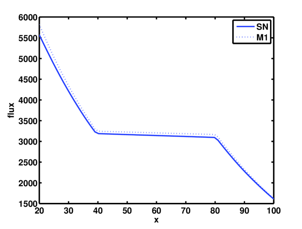
(a) Particle flux.

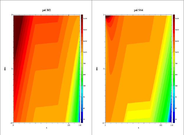
(b) Comparison of $M_{1}$ and benchmark distribution functions. Logarithmic scale.

Figure 3: Geometry with central void.

6.2 Two-dimensional Void-like Layer

Our second test case, again taken from [2], is a two-dimensional quadratic domain which contains a void-like layer, shown in gray in Figure 4(a). Again, we consider only elastic scattering modeled by the Henyey-Greenstein kernel.

We take $\sigma_{s}=0.5$ mm^-1 and $\sigma_{a}=0.005$ mm^-1 inside the square, and $\sigma_{s}=0.01$ mm^-1 and $\sigma_{a}=0.0001$ mm^-1 in the void-like ring. In both regions, $g=0$. An isotropic source of particles is placed on the left boundary. In a 2D contour plot (Figure 4), the fluxes $\psi^{0}$ from the discrete ordinate method and from the minimum entropy method are virtually indistinguishable. The propagation into the medium, as well as the void-like layer are equally well resolved. A difference between the models only becomes apparent in a logarithmic plot of a cut through the center of the square at $y=50$ mm. Figure 4 shows the particle flux along this line. The difference between both solutions is again of the order of one percent.

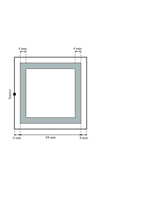
(a) Geometry containing void layer.

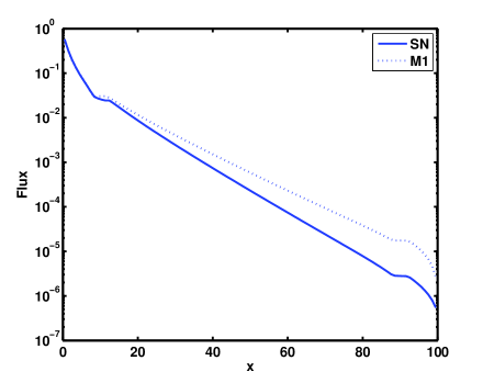
(b) Cut along $y=50$ mm.

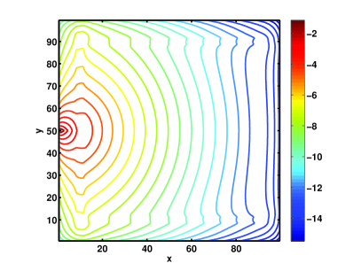
(c) Transport solution.

(d) Minimum entropy model.

Figure 4: Transport versus minimum entropy for void-like layer.

6.3 Electrons on Water Phantom

As a first test case that includes energy loss, we consider a 10 MeV electron beam impinging onto a slab of water. In Figure 5 we compare the results computed with our code to the dose computed by the state-of-the-art Monte Carlo code PENELOPE [32]. This code has been extensively validated against experimental results.

To obtain a good fit with the tabulated scattering data, we have fixed our model parameters for water as $\epsilon_{B}=16.0$ eV, $Z=9.40$, $\rho_{\rm el}=0.256\times 10^{23}$ g/cm³, $\rho_{\rm in}=6.21\times 10^{23}$ g/cm³. These parameters are directly inserted into the model (3), and subsequent derived models issued from (3). As boundary conditions, we have taken a very narrow Gaussian in energy, and a $\delta$ pulse in angle

$$\psi_{b}=\psi_{0}\exp(-200(\epsilon-\epsilon_{\rm beam})^{2})\delta(\mu-1),$$

and computed the angular moments. PENELOPE was set up in a pseudo-1D setting with a large beam size perpendicular to the beam direction.

In order to compare the different formulations of the models, both depth-dose curves in Figure 5 have been normalized to dose maximum one. The penetration depth computed with the $M_{1}$ model agrees very well with the Monte Carlo result. In fact this deviation is within the margin of differences between different Monte Carlo codes [33]. The only major difference occurs near the boundary, where the $M_{1}$ model overestimates the dose. This might be due to the simplified physics (possibly neglection of Bremsstrahlung effects) or an oversimplification of the angular dependence of $\psi$ in the $M_{1}$ model. Both possibilities will be investigated further. However, we believe that this result can serve as a proof of concept of a PDE based modeling of dose computation.

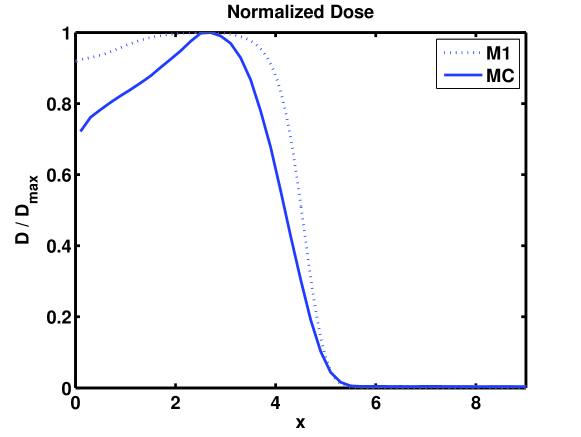
Figure 5: Dose for 10 MeV electron beam on water.

6.4 CT Data

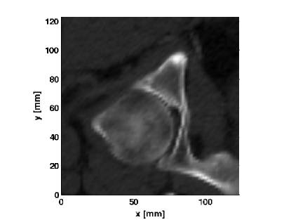
Figure 6: CT data of hip bone.

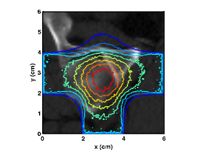
(a) Monte Carlo solution.

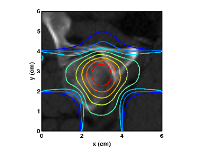
(b) Minimum entropy solution.

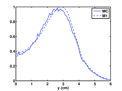
(c) Cut along $x=3$ cm.

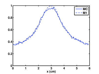
(d) Cut along $y=3$ cm.

Figure 7: Dose distribution for three beams impinging on hip bone.

In our final test case, we compare our method with Monte Carlo results from PENELOPE using real patient CT data showing the hip bone. We took a two-dimensional slice of $6\times 6$ cm from the three-dimensional CT data. A square region is split into 64$\times$64 squares. In each of the squares, the material is described by its Hounsfield grey value $\mathcal{G}(x,y)$. The grey values can be translated into physical parameters as follows,

$$\rho(x,y)=\left(\frac{\mathcal{G}(x,y)}{1000}+1\right)\rho_{\text{Water}},$$

i.e. the densities $\rho_{\rm el}$ and $\rho_{\rm in}$ for water are multiplied by a specified factor. The region shows the hip bone and the density varies between 86% and 226% of the value of water. The boundary conditions were set up similar to the previous case, with three beams of width 2 cm, each consisting of 10 MeV electrons, impinging from the centers of three sides of the domain. Contour plots of the dose distribution are shown in Figure 7. There, we also show two cuts through the dose distribution. looking at the 2D dose distribution, the contour lines agree very well. Note that, although we have used $3\times 10^{10}$ particles, there still is significant noise in the Monte Carlo results. The two cuts through the beam centers show that also quantitatively the independently computed dose distributions agree very well.

The computation time for the 3D Monte Carlo dose was $3\times 29$ hours for $3\times 10^{10}$ particles on a 3GHz Pentium 4 with 1 GB RAM. In 1D, the minimum entropy model took about 1 second, in 2D 4 seconds. Thus we expect a computation time of several seconds in a full 3D dose computation.

Again, this result shows that if our model is developed further, it may serve as an alternative to existing dose computation methods.

References

- [1] A. M. Anile, S. Pennisi, and M. Sammartino, A thermodynamical approach to Eddington factors, J. Math. Phys. 32 (1991), 544–550.
- [2] E. D. Aydin, C. R. E. Oliveira, and A. J. H. Goddard, A comparison between transport and diffusion calculations using finite element-spherical harmonics radiation transport method, Med. Phys. 29 (2002), 2013–2023.
- [3] P. Batten, N. Clarke, C. Lambert, and D. M. Causon, On the choice of wavespeeds for the HLLC riemann solver, SIAM J. Sci. Comput. 18 (1997), 1553–1570.
- [4] N. Bellomo and P. K. Maini, Preface (special issue on cancer modelling), Math. Mod. Math. Appl. Sci. 15 (2005), iii–viii.
- [5] , Preface (special issue on cancer modelling), Math. Mod. Math. Appl. Sci. 16 (2006), iii–vii.
- [6] , Preface (special issue on cancer modelling), Math. Mod. Math. Appl. Sci. 17 (2007), iii–vii.
- [7] C. Berthon, Stability of the MUSCL schemes for the Euler equations, Comm. Math. Sci. 3 (2005), 133–157.
- [8] C. Berthon, P. Charrier, and B. Dubroca, An HLLC scheme to solve the model of radiative transfer in two space dimensions, J. Sci. Comput. 31 (2007), 347–389.
- [9] C. Börgers, Complexity of Monte Carlo and deterministic dose-calculation methods, Phys. Med. Biol. 43 (1998), 517–528.
- [10] T. A. Brunner and J. P. Holloway, One-dimensional Riemann solvers and the maximum entropy closure, J. Quant. Spectrosc. Radiat. Transfer 69 (2001), 543–566.
- [11] C. Buet and B. Deprés, Asymptotic preserving and positive schemes for radiation hydrodynamics, J. Comput. Phys. 215 (2006), 717–740.
- [12] Y. Censor, Preface: Linear and nonlinear models and algorithms in intensity-modulated radiation therapy (IMRT), Lin. Alg. Appl. 428 (2008), 1203–1205.
- [13] J.-F. Coulombel, F. Golse, and T. Goudon, Diffusion approximation and entropy-based moment closure for kinetic equations, Asymptotic Analysis 45 (2005), 1–39.
- [14] B. Davison, Neutron transport theory, Oxford University Press, 1958.
- [15] B. Dubroca and J. L. Feugeas, Entropic moment closure hierarchy for the radiative transfer equation, C. R. Acad. Sci. Paris Ser. I 329 (1999), 915–920.
- [16] B. Dubroca and M. Frank, An iterative method for transport equations in radiotherapy, to appear in Proceedings of ECMI 08, 2009.
- [17] M. Frank, H. Hensel, and A. Klar, A fast and accurate moment method for dose calculation in electron radiotherapy, SIAM J. Appl. Math. 67 (2007), 582–603.
- [18] M. Frank and R. Pinnau, Existence, uniqueness and bounds for the half moment minimum entropy approximation to rediative heat transfer, Appl. Math. Lett. 20 (2007), 189–193.
- [19] K. A. Gifford, J. L. Horton Jr., T. A. Wareing, G. Failla, and F. Mourtada, Comparioson of a finite-element multigroup discrete-ordinates code with Monte Carlo for radiotherapy calculations, Phys. Med. Biol. 51 (2006), 2253–2265.
- [20] A. Harten, P.D. Lax, and B. van Leer, On upstream differencing and Godunov-type schemes for hyperbolic conservation laws, SIAM Rev. 25 (1983), 35–61.
- [21] C.D. Hauck, C.D. Levermore, and A.L. Tits, Convex duality in entropy-based moment closures: Characterizing degenerate densities, SIAM J. Control Optim. 47 (2008), 1977–2015.
- [22] H. Hensel, R. Iza-Teran, and N. Siedow, Deterministic model for dose calculation in photon radiotherapy, Phys. Med. Biol. 51 (2006), 675–693.
- [23] T. Goudon J.-F. Coulombel, Entropy-based moment closure for kinetic equations: Riemann problem and invariant regions, J. Hyperbolic Diff. Eq. 3 (2006), 649–672.
- [24] E. T. Jaynes, Information theory and statistical mechanics, Phys. Rev. 106 (1957), 620–630.
- [25] E. W. Larsen, M. M. Miften, B. A. Fraass, and I. A. D. Bruinvis, Electron dose calculations using the method of moments, Med. Phys. 24 (1997), 111–125.
- [26] C. Lehmann, Interaction of radiation with solids and elementary defect production, North Holland, 1977.
- [27] C. D. Levermore, Relating Eddington factors to flux limiters, J. Quant. Spectrosc. Radiat. Transfer 31 (1984), 149–160.
- [28] G. N. Minerbo, Maximum entropy Eddington factors, J. Quant. Spectrosc. Radiat. Transfer 20 (1978), 541–545.
- [29] N. F. Mott and H. S. W. Massey, The theory of atomic collisions, Clarendon Press, 1965.
- [30] I. Müller and T. Ruggeri, Rational extended thermodynamics, 2nd ed., Springer-Verlag, New York, 1993.
- [31] G. C. Pomraning, The Fokker-Planck operator as an asymptotic limit, Math. Mod. Meth. Appl. Sci. 2 (1992), 21–36.
- [32] F. Salvat, J.M. Fernandez-Varea, and J.Sempau, PENELOPE-2008, a code system for monte carlo simulation of electron and photon transport, OECD, 2008, ISBN 978-92-64-99066-1.
- [33] J. Sempau, S.J. Wilderman, and A.F. Bielajew, DPM - a fast, accurate Monte Carlo code optimized for photon and electron radiotherapy treatment planning dose computations, Phys. Med. Biol. 45 (2000), 2262–2291.
- [34] J. Tervo and P. Kolmonen, Inverse radiotherapy treatment planning model applying boltzmann-transport equation, Math. Models. Methods. Appl. Sci. 12 (2002), 109–141.
- [35] J. Tervo, P. Kolmonen, M. Vauhkonen, L. M. Heikkinen, and J. P. Kaipio, A finite-element model of electron transport in radiation therapy and related inverse problem, Inv. Probl. 15 (1999), 1345–1361.
- [36] J. Tervo, M. Vauhkonen, and E. Boman, Optimal control model for radiation therapy inverse planning applying the Boltzmann transport equation, Lin. Alg. Appl. 428 (2008), 1230–1249.
- [37] B. van Leer, Towards the ultimate conservative difference scheme V: A second-order sequel to Godunov’s method, J. Comput. Phys. 32 (1979), 101–136.
- [38] O.N. Vassiliev, T.A. Wareing, I.M. Davis, et al., Feasibility of a multigroup deterministic solution method for 3d radiotherapy dose calculations, Int. J. Radiat. Oncol. Biol. Phys. 72 (2009), 220–227.
- [39] C. D. Zerby and F. L. Keller, Electron transport theory, calculations and experiments, Nucl. Sci. Eng. 27 (1967), 190–218.