Two-phonon polaron resonances in self-assembled quantum dots

Abstract

We study the second-order polaronic resonance between 2-LO-phonon states and p-shell electron states in a quantum dot. We show that the spectrum in the resonance area can be quantitatively reproduced by a theoretical model. We propose also a perturbative approach to the problem based on a quasi-degenerate perturbation theory. This method not only considerably reduces the numerical complexity without considerable loss of accuracy but also gives some insight into the structure and origin of the resonance spectrum.

I Introduction

Carrier-phonon interaction is one of the major factors that determine the optical and transport properties of semiconductors. In semiconductor quantum dots, phonon-related effects manifest themselves in a special way due to the discrete spectrum of carriers confined in these structures. On the one hand, such a discrete density of states may slow down carrier relaxation bockelmann90 ; urayama01 ; heitz01 . On the other hand, coupling of a confined charge system to the nearly dispersionless (thus, also spectrally discrete) system of longitudinal optical (LO) phonons leads to the formation of correlated carrier-phonon states hameau99 ; verzelen02a and to a reconstruction of the system spectrum, as observed, e.g., in intraband absorption experiments hameau99 ; hameau02 . This effect is a generalized form of a polaron, known from bulk systems.

Apart from the (unmeasurable) energy shifts accompanying the polaron formation, this effect manifests itself by the appearance of polariton-like resonances (anticrossings) between the essentially discrete zero-phonon and 1- or 2- phonon states whenever the energy difference between two carrier states matches the energy of one or two LO phonons hameau02 . The 2-phonon resonance is of particular interest since the 2-LO-phonon energy of about 70 meV falls into the range of typical separations between electron energy levels in self-assembled structures.

Understanding such coherent effects in the carrier-phonon coupling in quantum dots is essential not only for the correct description of the system spectrum but also for the discussion of relaxation properties. In particular, the strong coupling between the confined carriers and LO phonons precludes purely LO-phonon-mediated relaxation but opens new channels of efficient two-phonon (acoustic + optical) emission verzelen00 ; jacak02a ; grange07 , which may explain efficient carrier relaxation observed in some experiments heitz97 ; ignatiev01 ; zibik04 .

Far from the degeneracy (resonance) point, the coupling to LO phonons may be treated perturbatively. Also a first-order polaronic resonance does not present serious difficulties, as it involves only a zero-phonon state and a one-phonon state. These two states are directly coupled by the Fröhlich interaction Hamiltonian and the resulting resonant anticrossing can be treated, e.g., by a second-order Wigner–Brillouin perturbation theory wendler93a ; wendler93b . In contrast, the second-order resonance, involving a zero-phonon state and a two-phonon state is more complex, since the observed anticrossing is due to higher-order, indirect couplings via other states. In this case one resorts to a numerical treatment hameau99 ; hameau02 ; jacak03b ; obreschkow07 ; stauber00 . The latter is feasible due to the discrete (dispersionless) character of the LO modes, which allows one to describe the LO phonon subsystem by a finite set of either orthogonal stauber00 or non-orthogonal obreschkow07 collective modes. The numerical approach to the polaron problem turns out to successfully reproduce the qualitative features. However, the early attempts to model the experimental results hameau99 ; hameau02 suggested that certain material parameters must be adjusted in order to achieve a quantitative agreement with the measurement data. This seemed plausiblejacak02f as QDs are inherently inhomogeneous systems the quantitative properties of which may depend, e.g., on the size and composition characteristics. Such a viewpoint would mean, however, that a full understanding and quantitative description of the carrier–LO phonon interaction in QDs may not be possible.

The goal of the present paper is twofold. First, we discuss the spectrum of the electron-LO-phonon system in the vicinity of the two-phonon resonance, including the effects of QD asymmetry (ellipticity), non-parabolicity of the confinement potential, as well as the external magnetic field. We show that the experimentally observed spectrum of the coupled electron-LO-phonon system can be successfully reproduced using only standard material constants, without any adjustable parameters. In this way we show that the existing theorystauber00 ; hameau02 does allow us to understand the physics of carrier–LO phonon interactions in QDs completely and quantitatively. We calculate also the intraband (far infra-red) absorption spectrum of a QD ensemble, where the polaronic resonance is clearly manifested. Second, we present an effective Hamiltonian approach, based on the quasi-degenerate perturbation theory which reduces the problem size from a few thousands of basis states to just a few and provides some insight into the structure of two-phonon polaron states. This, in turn, demonstrates that describing the electron–LO phonon system does not necessarily have to involve heavy numerics and may open the way to the efficient description of even higher-order effects.

The paper is organized as follows: First, in Sec. II, we recall the model of an electron confined in a QD interacting with LO phonons. Then in Sec. III, numerical approach is described. The spectrum of a single QD, as well as absorption on a QD ensemble and the magnetopolaron spectrum are presented in Sec. IV. The two following sections V and VI describe the effective Hamiltonian approach and present results obtained within this method.

II The model

We consider a self-assembled quantum dot occupied by a single electron. The effective confinement potential in the $xy$ plane is assumed to be almost axially symmetric and parabolic, although small corrections accounting for ellipticity and non-parabolicity will be taken into account. In the $z$ (growth) direction, the confinement is assumed to be much stronger, as is typical for these structures. The electron confined in the QD is coupled to the polarization field associated with the LO phonons. In calculations, GaAs parameters will be used.

The system is described by the Hamiltonian

$$H=H_{0}+H_{\mathrm{a}}+H_{\mathrm{np}}+H_{\mathrm{int}}+H_{\mathrm{ph}},$$ (1)

where $H_{0}$ describes an electron in an isotropic dot, $H_{\mathrm{a}}$ and $H_{\mathrm{np}}$ account for the anisotropy (ellipticity) and non-parabolicity of the confinement potential, respectively, $H_{\mathrm{int}}$ describes the electron-phonon coupling and $H_{\mathrm{ph}}$ is the free LO phonon Hamiltonian.

The first term in Eq. (1) is jacak98a

$$H_{0}=\frac{1}{2m^{*}}\left({\bm{p}}-e{\bm{A}}\right)^{2}+\frac{1}{2}m^{*}\omega_{0}^{2}r_{\bot}^{2}+\frac{1}{2}m^{*}\omega_{z}^{2}z^{2}$$

and describes an electron in an axially symmetric harmonic potential in a magnetic field $B$ oriented along the symmetry axis, where $m^{*}=0.066m_{\mathrm{e}}$ is the effective mass of an electron in GaAs and $\bm{r_{\bot}}$ denotes the in-plane component of the electron position. The energy $\hbar\omega_{0}$ is the level spacing for in-plane excitations in the absence of magnetic fields. We will refer to this quantity as the characteristic energy of the system and use it as a system parameter in the discussion that follows. This energy parameter is related to the in-plane confinement length $l_{0}=\sqrt{\hbar/(m^{*}\omega_{0})}$. The confinement along the $z$ axis is much stronger than that in the $xy$ plane, that is, $\omega_{z}\gg\omega_{0}$. The dynamics along this strongly confined direction is restricted to the lowest subband, corresponding to the ground state wave function

$$\Phi_{z}(z)=\frac{1}{\sqrt{l_{z}}{\pi}^{1/4}}e^{-\frac{z^{2}}{2l_{z}^{2}}},$$

where $l_{z}=\sqrt{\hbar/(m^{*}\omega_{z})}$ is the confinement length in this direction. Since the dots we intend to model have the height to diameter ratio of about 10 (Ref. hameau02, ) we choose $l_{z}=0.1l_{0}$, which will be fixed throughout the paper.

The essential part of $H_{0}$, accounting for the dynamics in the $xy$ plane, is the well known Fock–Darwin Hamiltonian describing a 2-dimensional harmonic oscillator in a perpendicular magnetic field. We choose the symmetric gauge, ${\bm{A}}=\frac{1}{2}(-By,Bx,0)$, where B is the magnetic field, and use the basis of eigenstates of this Hamiltonian (Fock–Darwin states jacak98a ), denoted as $|nm\rangle$, where $n=0,1,\ldots$ and $m=\ldots,-1,0,1,\ldots$ are the radial and angular momentum quantum numbers, respectively (that is, $\hbar m$ is the projection of the angular momentum on the symmetry axis $z$). The corresponding wave functions are

$$\Psi_{nm}(\bm{r_{\bot}})=\langle\bm{r_{\bot}}|nm\rangle=$$

$$\frac{\sqrt{2}}{l_{B}}\sqrt{\frac{n!}{(n+|m|)!}}\left(\frac{r_{\bot}}{l_{B}}\right)^{|m|}e^{-\frac{r_{\bot}^{2}}{2l_{B}^{2}}}\mathcal{L}^{|m|}_{n}\left(\frac{r_{\bot}^{2}}{l_{B}^{2}}\right),$$

where $\mathcal{L}^{|m|}_{n}\left(s\right)$ is a Laguerre polynomial. Here $l_{\mathrm{B}}=\sqrt{\hbar/(m^{*}\omega_{\mathrm{B}})}$ is the in-plane confinement width in the magnetic field, where $\omega_{\mathrm{B}}^{2}=\omega_{0}^{2}+\omega_{\mathrm{c}}^{2}/4$ and $\omega_{\mathrm{c}}=eB/m^{*}$ is the cyclotron frequency in the magnetic field $B$. In the Fock–Darwin basis, the Hamiltonian is

$$H_{0}=\sum_{nm}\epsilon_{nm}|nm\rangle\!\langle nm|,$$

where

$$\epsilon_{nm}=\hbar\omega_{\mathrm{B}}(2n+|m|+1)-\frac{1}{2}\hbar\omega_{\mathrm{c}}m.$$

The second term in Eq. (1) describes a weak anisotropy (ellipticity) of the confinement potential and has the form jacak03a

$$H_{\mathrm{a}} = \frac{\beta}{2}m^{*}\omega_{0}^{2}(x^{2}-y^{2})$$

$$= \frac{\beta}{2}\frac{\hbar\omega_{0}^{2}}{\omega_{\mathrm{B}}}\sum_{nm,n^{\prime}m^{\prime}}V_{(nm)(n^{\prime}m^{\prime})}|nm\rangle\!\langle n^{\prime}m^{\prime}|,$$

where $\beta$ is a dimensionless parameter and the non-vanishing matrix elements in the basis of Fock–Darwin states are

$$V_{(0\bar{2})(00)}=\frac{\sqrt{2}}{2},\quad V_{(0\bar{2})(10)}=\sqrt{2},\quad V_{(0\bar{1})(01)}=1,$$

with the symmetries $V_{(nm)(n^{\prime}m^{\prime})}=V_{(n^{\prime}m^{\prime})(nm)}=V_{(n\bar{m})(n^{\prime}\bar{m^{\prime}})}$. Here and throughout the paper, a bar over a number denotes a minus sign. This anisotropy term leads to the splitting of the $p$-shell states (in zero magnetic field) given by $\Delta E_{p}=\beta\hbar\omega_{0}$ which can be read off the spectral position of the $p$-shell states.

The third part in Eq. (1) accounts for non-parabolicity of the confining potential

$$H_{\mathrm{np}}=-\frac{1}{2}\hbar\omega_{0}\chi\left(\frac{r_{\bot}}{l_{0}}\right)^{4},$$

where $l_{0}$ is the in plane confinement length in the absence of magnetic field and $\chi\ll 1$ is a positive parameter defining the strength of non-parabolicity.

In the basis of Fock–Darwin states, the non-parabolicity term reads

$$H_{\mathrm{np}}=-\chi\hbar\omega_{0}\sum_{(n,m)(n^{\prime}m^{\prime})}\mathcal{V}_{(nm)(n^{\prime}m^{\prime})}|nm\rangle\!\langle n^{\prime}m^{\prime}|,$$

where non-vanishing matrix elements are

$$\mathcal{V}_{(00)(00)} = 4,$$

$$\mathcal{V}_{(00)(10)}=\mathcal{V}_{(10)(0,0)} = 8,$$

$$\mathcal{V}_{(01)(01)}=\mathcal{V}_{(0\bar{1})(0\bar{1})} = 12,$$

$$\mathcal{V}_{(02)(02)}=\mathcal{V}_{(0\bar{2})(0\bar{2})} = 24,$$

$$\mathcal{V}_{(10)(10)} = 28.$$

The electron-phonon coupling Hamiltonian has the form jacak03a

$$H_{\mathrm{int}}=\sum_{nmn^{\prime}m^{\prime}}|nm\rangle\!\langle n^{\prime}m^{\prime}|\sum_{\bm{k}}F_{(nm)(n^{\prime}m^{\prime})}(\bm{k})b_{\bm{k}}+\mathrm{H.c},$$

where

$$F_{(nm)(n^{\prime}m^{\prime})}(\bm{k})=$$

$$\sqrt{\frac{\hbar\Omega}{2v\varepsilon_{0}\tilde{\varepsilon}}}\frac{e}{k}f_{(nm)(n^{\prime}m^{\prime})}(q)e^{-q^{2}-\xi^{2}}e^{i(m^{\prime}-m)\phi}.$$

Here we write the wave vector as $\bm{k}=(k_{\bot}\cos\phi,k_{\bot}\sin\phi,k_{z})$ and introduce the short-hand notation $q=k_{\bot}l_{\mathrm{B}}/2$, $\xi=k_{z}l_{z}/2$; $\Omega$ is the frequency of LO phonons at $\bm{k}=0$ ($\hbar\Omega=36.7~{}\mathrm{meV}$), $v$ is the normalization volume for the phonon modes, $\varepsilon_{0}$ is the vacuum permittivity, and $\tilde{\varepsilon}=(1/{\varepsilon_{\infty}}-1/{\varepsilon_{\mathrm{s}}})^{-1}=70.3$ is the effective dielectric constant (again, the values correspond to GaAs). Note that the Gaussian cut-off at $k\sim 1/l_{\mathrm{B}}$ restricts the coupling only to long-wavelength modes, so the frequency of LO phonons can be replaced by its value at the center of the Brillouin zone (dispersionless approximation). The coupling functions have the general symmetry

$$F_{(nm)(n^{\prime}m^{\prime})}(\bm{k})=F^{*}_{(n^{\prime}m^{\prime})(nm)}(-\bm{k}),$$

while the $f$ functions for our choice of basis states satisfy

$$f_{(nm)(n^{\prime}m^{\prime})}(q)=f_{(n^{\prime}m^{\prime})(nm)}(q)=f_{(n^{\prime}\bar{m}^{\prime})(n\bar{m})}(q).$$ (2)

The functions $f_{(nm)(n^{\prime}m^{\prime})}(q)$ are listed in Tab. 1. It may be interesting to note that the functions $F$ are not linearly independent. This follows, e.g., from the linear dependence of the subset of $f$ functions $\{f_{(00)(00)},f_{(01)(01)},f_{(10)(00)}\}$, all of which correspond to $m^{\prime}-m=0$. The lack of linear independence reduces the number of collective modes needed to represent the system.

$$\begin{array}[]{|l|*{4}{c}|}nm&00&01&10&02\\ \hline\cr 00&1&-iq&-q^{2}&-q^{2}/\sqrt{2}\\ 0\bar{1}&-iq&-q^{2}&i(q^{3}-q)&iq^{3}/\sqrt{2}\\ 01&-iq&1-q^{2}&i(q^{3}-q)&i(q^{3}-2q)/\sqrt{2}\\ 10&-q^{2}&i(q^{3}-q)&1-2q^{2}+q^{4}&(q^{4}-2q^{2})/\sqrt{2}\\ 0\bar{2}&-q^{2}/\sqrt{2}&iq^{3}/\sqrt{2}&(q^{4}-2q^{2})/\sqrt{2}&q^{4}/2\\ 02&-q^{2}/\sqrt{2}&i(q^{3}-2q)/\sqrt{2}&(q^{4}-2q^{2})/\sqrt{2}&1-2q^{2}+q^{4}/2\\ \end{array}$$

Table 1: Functions $f_{(nm)(n^{\prime}m^{\prime})}(q)$ used in the definition of the coupling constants. Functions not listed here can be found using Eq. (2).

The last contribution to the Hamiltonian,

$$H_{\mathrm{ph}}=\hbar\Omega\sum_{\bm{k}}b_{\bm{k}}^{{\dagger}}b_{\bm{k}}$$

describes free, dispersionless LO phonons.

III The numerical approach

In this Section, we describe the general framework for the numerical diagonalization of the carrier-phonon Hamiltonian. Then, in Section IV we present the results for a few classes of systems.

$$\begin{array}[]{|l|*{3}{c}|}&\alpha=A&\alpha=B&\alpha=C\\ \hline\cr M=0&-q^{2}/\sqrt{x_{4}}&\frac{x_{4}q^{4}-x_{6}q^{2}}{\sqrt{x_{4}^{2}x_{8}-x_{4}x_{6}^{2}}}&(1-a_{2}q^{2}+a_{4}q^{4})/\sqrt{c}\\ M=\pm 1&iq/\sqrt{x_{2}}&\frac{i(x_{2}q^{3}-x_{4}q)}{\sqrt{x_{6}x_{2}^{2}-x_{4}^{2}x_{2}}}&\\ M=\pm 2&-q^{2}/\sqrt{x_{4}}&\frac{x_{4}q^{4}-x_{6}q^{2}}{\sqrt{x_{4}^{2}x_{8}-x_{4}x_{6}^{2}}}&\\ M=\pm 3&iq^{3}/\sqrt{x_{6}}&&\\ M=\pm 4&q^{4}/\sqrt{x_{8}}&&\end{array}$$

Table 2: Functions $\phi_{M\alpha}(q)$ used in the definition of collective modes.

Our approach to the diagonalization of the Hamiltonian (1) is based on the collective mode representation of the LO phonons stauber00 . We use the basis of the electron subsystem composed of up to 6 lowest Fock–Darwin states (3 lowest energy shells, $2n+|m|+1\leq 3$). For this truncated basis, we define 14 collective phonon modes which are needed to exactly represent the carrier-phonon coupling in the dispersionless approximation,

$$B_{M\alpha}=\sqrt{\frac{l_{\mathrm{B}}}{v}}\sum_{k}\frac{1}{k}\phi_{M\alpha}(q)e^{-q^{2}-\xi^{2}+iM\phi}b_{k},$$ (3)

where $\alpha=A,B,C$ labels different modes with the same angular momentum $M$ and the functions $\varphi_{M\alpha}(q)$ are listed in Tab. 2. For an axially symmetric dot, the appropriate functions are expressed in terms of the shape-dependent parameters (defined for $l$ even)

$$x_{l}=\frac{1}{4\pi^{3}}\int d^{3}q\frac{q_{\bot}^{l}}{q^{2}}\exp\left[-2\left(q_{\bot}^{2}+\frac{l_{z}^{2}}{l_{\mathrm{B}}^{2}}q_{z}^{2}\right)\right].$$

We define also

$$a_{2} = \frac{x_{2}x_{4}x_{8}-x_{4}^{2}x_{6}}{{x_{4}^{2}x_{8}-x_{4}x_{6}^{2}}},$$

$$a_{4} = \frac{x_{2}x_{4}x_{6}-x_{4}^{3}}{{x_{4}^{2}x_{8}-x_{4}x_{6}^{2}}},$$

$$c = x_{0}-2a_{2}x_{2}+2a_{4}x_{4}+a_{2}^{2}x_{4}-2a_{2}a_{4}x_{6}+a_{4}^{2}x_{6}.$$

The numbers $x_{l}$ can be found exactly in the limit of a strong vertical confinement, $l_{z}/l_{\mathrm{B}}\to 0$,

$$x_{l}\to\frac{(l-1)!!}{2^{l+2}\sqrt{2\pi}}.$$

These limiting values are collected in Tab. 3 and compared with those for $l_{z}/l_{\mathrm{B}}=0.1$. The leading order correction is $O(l_{z}^{2}/l_{\mathrm{B}}^{2})$.

$$\begin{array}[]{|c|r *{1}{c}|}&\lx@intercol\hfil~{}~{}l_{z}/l_{\mathrm{B}}=0{}{}\hfil\lx@intercol&~{}~{}l_{z}/l_{\mathrm{B}}=0.1{}{}\\ \hline\cr x_{2}&\frac{1}{16\sqrt{2\pi}}\approx 0.0249&0.0221\\ x_{4}&\frac{3}{64\sqrt{2\pi}}\approx 0.0187&0.0159\\ x_{6}&\frac{15}{266\sqrt{2\pi}}\approx 0.0234&0.0193\\ x_{8}&\frac{105}{1024\sqrt{2\pi}}\approx 0.0409&0.0329\\ \end{array}$$

Table 3: Comparison between numbers $x_{l}$ calculated for strong confinement limit $l_{z}/l_{\mathrm{B}}\to 0$ and for a realistic value $l_{z}/l_{\mathrm{B}}=0.1$ at $B=0$.

With the definition (3), the collective operators $B_{M\alpha},B^{{\dagger}}_{M\alpha}$ satisfy the usual bosonic commutation relations, $[B_{M\alpha},B^{{\dagger}}_{M^{\prime}\alpha^{\prime}}]=\delta_{MM^{\prime}}\delta_{\alpha\alpha^{\prime}}$ (that is, we follow the standard approach of orthogonalized modes stauber00 , although an alternative approach is also possible obreschkow07 ). In terms of the collective modes, the interaction Hamiltonian reads

$$H_{\mathrm{int}} = \sqrt{\frac{\hbar\Omega e^{2}}{2l_{B}\varepsilon_{0}\tilde{\varepsilon}}}\sum_{nmn^{\prime}m^{\prime}}\sum_{\alpha}|nm\rangle\!\langle n^{\prime}m^{\prime}|$$

$$\times\gamma_{(nm)(n^{\prime}m^{\prime})\alpha}B_{m^{\prime}-m,\alpha}+\mathrm{H.c.},$$

where the coupling constants $\gamma_{(nm)(n^{\prime}m^{\prime})\alpha}$ are collected in Tab. 4. The mode $B_{0\mathrm{C}}$ couples only to the unit operator on the restricted electron subspace, $\mathbb{I}=\sum_{mn}|mn\rangle\!\langle mn|$, and can be discarded from the discussion stauber00 .

$$\begin{array}[]{|r|*{4}{c}|}nm~{}\alpha&00&01&10&02\\ \hline\cr 00~{}A&(a_{4}x_{6}-a_{2}x_{4})/\sqrt{x_{4}}&-\sqrt{x_{2}}&\sqrt{x_{4}}&\sqrt{x_{4}/2}\\ B&{-a_{4}\sqrt{x_{8}-{x_{6}^{2}}/{x_{4}}}}&&&\\ C&\sqrt{c}&&&\\ 0\bar{1}~{}A&-\sqrt{x_{2}}&\sqrt{x_{4}}&({x_{4}}/{x_{2}}-1)\sqrt{x_{2}}&\sqrt{x_{6}/2}\\ B&&&{\sqrt{x_{6}-{x_{4}^{2}}/{x_{2}}}}&\\ 01~{}A&-\sqrt{x_{2}}&a_{4}x_{6}/\sqrt{x_{4}}-(a_{2}+1)\sqrt{x_{4}}&{{{x_{4}}}/{\sqrt{x_{2}}}-\sqrt{x_{2}}}&{{x_{4}}/{\sqrt{2x_{2}}}-\sqrt{2x_{2}}}\\ B&&-a_{4}\sqrt{x_{8}-{x_{6}^{2}}/{x_{4}}}&{\sqrt{x_{6}-{x_{4}^{2}}/{x_{2}}}}&{\sqrt{{x_{6}}/{2}-{x_{4}^{2}}/{2x_{2}}}}\\ C&&\sqrt{c}&&\\ 10~{}A&\sqrt{x_{4}}&{{x_{4}}/{\sqrt{x_{2}}}-\sqrt{x_{2}}}&(2-a_{2})\sqrt{x_{4}}+(a_{4}-1)x_{6}/\sqrt{x_{4}}&{\sqrt{2x_{4}}-{x_{6}}/{\sqrt{2x_{4}}}}\\ B&&{\sqrt{x_{6}-{x_{4}^{2}}/{x_{2}}}}&{(1-a_{4})}/{x_{4}}\sqrt{x_{8}-{x_{6}^{2}}/{x_{4}}}&{\sqrt{{x_{8}}/{2}-{x_{6}^{2}}/{2x_{4}}}}\\ C&&&\sqrt{c}&\\ 0\bar{2}~{}A&\sqrt{x_{4}/2}&{\sqrt{x_{6}/2}}&{\sqrt{2x_{4}}-{x_{6}}/{\sqrt{2x_{4}}}}&\sqrt{x_{8}}/2\\ B&&&{\sqrt{{x_{8}}/{2}-{x_{6}^{2}}/{2x_{4}}}}&\\ 02~{}A&\sqrt{x_{4}/2}&{{x_{4}}/{\sqrt{2x_{2}}}-\sqrt{2x_{2}}}&\sqrt{2x_{4}}-{x_{6}}/{\sqrt{2x_{4}}}&(2-a_{2})\sqrt{x_{4}}+(a_{4}-\frac{1}{2})x_{6}/\sqrt{x_{4}}\\ B&&{\sqrt{{x_{6}}/{2}-{x_{4}^{2}}/{2x_{2}}}}&{\sqrt{{x_{8}}/{2}-{x_{6}^{2}}/{2x_{4}}}}&\sqrt{x_{8}-x_{6}^{2}/x_{4}}(\frac{1}{2}-a_{4})/x_{4}\\ C&&&&\sqrt{c}\\ \end{array}$$

Table 4: Coupling constants $\gamma_{(nm)(n^{\prime}m^{\prime})\alpha}$ for the collective LO modes. Definitions as in Tab. 2. The values not listed in the table can be reproduced form the relation $\gamma_{(n\bar{m})(n^{\prime}\bar{m}^{\prime})\alpha}=\gamma_{(nm)(n^{\prime}m^{\prime})\alpha}.$

The Hamiltonian (1) is then diagonalized numerically, including states with up to 3 phonons, which yields a computational basis of 4080 states. The relevance of 4-phonon states is discussed in the Appendix.

IV Numerical Results

In this section, we present the results of a numerical investigation on the second-order resonant polarons. First, we study the system in the absence of a magnetic field. We calculate the system spectrum as a function of the separation between the unperturbed electron energy levels (that is, indirectly, on the QD size). We model also the intraband absorption spectrum of an inhomogeneously broadened ensemble of QDs, where the polaron resonance is clearly manifested. Next, we calculate the spectrum of a single QD with a fixed size as a function of an external axial magnetic field and compare the results to the existing experimental data.

When plotting the obtained polaron spectra, we present only the states with a sufficient transition probability, that way spurious uncoupled states (for the truncation at the 3-phonon level) are not included. Since we focus on the second-order resonance, all important couplings are contained in the model.

IV.1 Size-dependent polaron spectrum

We first consider the system without a magnetic field and focus on the resonance between the unperturbed excited electronic states $|0\pm 1\rangle$ and a set of two-phonon states $|00,2\mathrm{ph}\rangle$. Here and throughout the paper notation of this form stands for all two-phonon states with the electronic part in the ground state: $|00\rangle_{\mathrm{el}}\otimes(B_{M\alpha}^{\dagger}B_{M^{\prime}\alpha^{\prime}}^{\dagger}|0\rangle_{\mathrm{ph}})$. Any other group of states with different number of phonons is denoted in a similar way. The quantities of interest in the present calculation are energies of the system eigenstates and the photon absorption probability for an intraband transition between the ground state and a given excited state. The former are obtained directly for the numerical diagonalization, while the latter, for an excited state $|\kappa\rangle$, is calculated according to

$$|\mu_{\kappa}|^{2}=\left|\langle\kappa|\hat{d}^{(-)}_{\lambda}|\Psi_{\mathrm{G}}\rangle\right|^{2},$$ (4)

where $\Psi_{G}$ denotes the numerically calculated ground state and $\hat{d}^{(-)}_{\lambda}$ is the negative frequency part of the dipole moment operator, which depends on the polarization $\lambda$ of the optical wave exciting the system. For the $\sigma_{\pm}$ circular polarizations one has (upon truncation to our computational space)

$$\hat{d}^{(-)}_{+} \propto (|01\rangle\!\langle 00|+\sqrt{2}|02\rangle\!\langle 01|+|10\rangle\!\langle 0\bar{1}|+|01\rangle\!\langle 10|$$

$$+\sqrt{2}|0\bar{1}\rangle\!\langle 0\bar{2}|+|00\rangle\!\langle 0\bar{1}|)\otimes\mathbb{I}_{\mathrm{ph}}$$

and

$$\hat{d}^{(-)}_{-} \propto (|0\bar{1}\rangle\!\langle 00|+\sqrt{2}|0\bar{2}\rangle\!\langle 0\bar{1}|+|10\rangle\!\langle 01|+|0\bar{1}\rangle\!\langle 10|$$

$$+\sqrt{2}|01\rangle\!\langle 02|+|00\rangle\!\langle 01|)\otimes\mathbb{I}_{\mathrm{ph}},$$

where $\mathbb{I}_{\mathrm{ph}}$ is the identity operator on the phonon subsystem. For the linear polarization along the $x$ and $y$ axes, the dipole moment operator is

$$\hat{d}^{(-)}_{x}\propto d^{(-)}_{+}+d^{(-)}_{-},\quad\hat{d}^{(-)}_{y}\propto d^{(-)}_{+}-d^{(-)}_{-}.$$

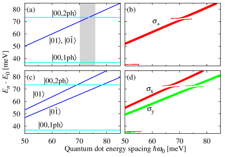
Figure 1: (a,c) Dependence of the unperturbed eigenenergies (without electron-phonon coupling) on characteristic energy of the QD. (b,d) The QD energy spectrum with electron-phonon interaction included. Panels (a) and (b) refer to a cylindrically symmetric dot, while (c) and (d) present the spectra for an elliptical dot. In (b) and (d) the line thickness is proportional to the intraband transition probability $|\mu_{k}|^{2}$, the lines are labeled by the polarization of the exciting light. Only states for which $|\mu_{k}|^{2}>0.1$ are plotted.

We investigate two cases: an isotropic QD and an anisotropic one (Fig. 1). In Figs. 1(a) and 1(c), we have presented states from the $p$ shell without phonons as well as one-phonon and two-phonon states with the electronic part in the ground state ($|00,1\mathrm{ph}\rangle$, $|00,2\mathrm{ph}\rangle$). The energies are shown relative to the system ground state. All the other unperturbed states lie in a higher energy range. In the case of an isotropic dot, in the absence of the electron-phonon coupling, for a certain value of the electron level spacing (shaded area in Fig. 1a), $p$-shell states ($|0\pm 1\rangle$) intersect with the group of two-phonon states with the electron in its ground state ($|00,2\mathrm{ph}\rangle$).

When the electron-phonon coupling is included, this intersection turns into an avoided crossing pattern, as shown for an isotropic dot in Fig. 1(b). Importantly, there are no direct matrix elements coupling those states and the coupling between the $p$-shell zero-phonon states and the two-phonon states is mediated through one-phonon states. Even though this coupling is of the second order the anticrossing is quite strong and its width is 1.75 meV.

If anisotropy is included, the degeneracy of states $|01\rangle$ and $|0\bar{1}\rangle$ is lifted and two lines in the polaron spectrum are observed for different linear polarizations of the incident light. As can be seen on Figs. 1(c) and 1(d), there are two intersections [Fig. 1(c)] resulting in two anticrossings [Fig. 1(d)] which become visible in the absorption spectrum depending on the polarization.

In the low energy range [36 meV, Figs. 1(b), 1(d)] states with small but noticeable transition probability can be observed. Their existence is due to the first order coupling leading to some transfer of the oscillator strength from the $p$-shell states to 1-phonon states $|00,1\mathrm{ph}\rangle$.

The position of the resonance in Figs. 1(b) and 1(d) is shifted with respect to the intersection of decoupled states [Figs. 1(a) and 1(c)]. The center of the resonance for the interacting case is located at a lower QD energy spacing (71 meV) than the intersection point between non-interacting states $|00,2\mathrm{ph}\rangle$ and $|0\pm 1\rangle$ (73.4 meV). Such a behaviour results from the presence of other states directly coupled to zero- and two- phonon lines. The most important states influencing the position of the resonance are 3-phonon states $|00,3\mathrm{ph}\rangle$ which are relatively close to the $|00,2\mathrm{ph}\rangle$ states and effectively reduce their energy.

Since the second-order resonance is relatively strong it should also be visible in the absorption spectra of inhomogeneously broadened ensembles. This is discussed in Sec. IV.2. More insight to the structure of the second-order resonant polarons can be obtained using the effective Hamiltonian approach which is presented in Sec. VI.

IV.2 Polaron resonance in the ensemble absorption

In this section, intraband absorption spectra of an inhomogeneously broadened QD ensemble are calculated. QD sizes in self–assembled QD ensembles are always given by some distribution. We take this inhomogeneity of sizes into account and theoretically investigate the ensemble intraband absorption spectrum in the area of the two phonon resonance.

The QDs are parametrized by their energy spacing $\hbar\omega_{0}^{(i)}$, where $i$ labels dots in the ensemble. The distribution of QD energies is assumed to be described by a Gaussian function

$$f_{\overline{\epsilon},\sigma}(\hbar\omega_{0}^{(i)})=\frac{1}{\sigma\sqrt{2\pi}}e^{-\frac{(\hbar\omega_{0}^{(i)}-\overline{\epsilon})^{2}}{2\sigma^{2}}},$$

where $\overline{\epsilon}=\hbar\overline{\omega_{0}}$ and $\sigma$ are the mean transition energy and its standard deviation, respectively. Those parameters will be chosen in such a way that the second order resonance is located in the high-energy tail of the QD size distribution.

In order to construct high quality absorption spectra, we calculate the polaronic states for up to $N=10^{5}$ QDs with the transition energies $\hbar\omega_{0}^{(i)}$ uniformly distributed over a sufficiently broad range. From these numerical results, the absorption spectrum for the requested polarization is calculated according to

$$I(\hbar\omega)\propto\sum_{i=1}^{N}\sum_{\kappa=1}^{N_{\mathrm{ev}}}\delta(\hbar\omega-\mathcal{E}_{i\kappa})|\mu_{\kappa}|^{2}f_{\overline{\epsilon},\sigma^{2}}(\hbar\omega_{0}^{(i)}),$$

where $\hbar\omega$ is the energy of the absorbed photon, $N$ and $N_{\mathrm{ev}}$ are the number of QDs used in calculations and the number of eigenvalues for $i$–th QD, respectively, ${\mathcal{E}_{i\kappa}}$ stands for $\kappa$–th eigenenergy of $i$–th quantum dot and $|\mu_{\kappa}|^{2}$ is given by Eq. (4).

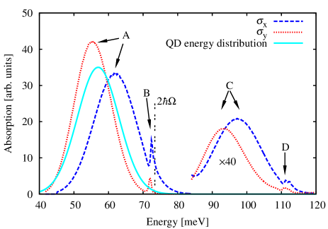
Figure 2: (Color online) Absorption spectra for two different linear polarizations ($\sigma_{X}$, $\sigma_{Y}$) with anisotropy and without non-parabolic corrections. Distribution of characteristic energies $\hbar\omega_{0}^{(i)}$ is also presented. The mean energy and its standard deviation are taken respectively as $\hbar\overline{\omega_{0}}=57~{}\mathrm{meV}$ and $\sigma=6~{}\mathrm{meV}$. Labels denote features discussed in the text. The dotted vertical line marks the 2-LO phonon energy. The right part of the plot is scaled up, as marked.

The absorption spectrum in the case of a polaron in an anisotropic, parabolic confinement potential is presented in Fig. 2. The polaronic feature is clearly manifested for energies close to the energy of two LO phonons (feature B in the plot). Additionally, a phonon replica (C) of the main absorption peak is visible for higher energies, including the resonance feature (D). The latter is slightly broadened and consists of two peaks (D). It is worth mentioning that the main absorption feature (A), the resonant feature (B), as well as the phonon-replica (C) are reproduced correctly in a diagonalization with up to 3-phonon states included. On the other hand, the replica of the resonant feature (D) is modelled correctly only if 4-phonon states are taken into account (see Appendix A). The absorption features for the $\sigma_{X}$ and $\sigma_{Y}$ polarizations are not related by symmetry with respect to the average QD energy ($\overline{\epsilon}$). This effect is due to coupling to a lower lying group of one-phonon states, which moves the relevant eigenvalues to higher energies.

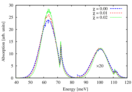
Figure 3: (Color online) Absorption spectra on ensembles of isotropic QDs for different non-parabolic corrections. Standard deviation $\sigma=6~{}\mathrm{meV}$, the mean energy $\hbar\overline{\omega_{0}}=62$, $67.1$ and $72.8~{}\mathrm{meV}$ respectively for ascending values of $\chi$.

The position of the second-order polaronic feature is slightly lower than the energy of two LO phonons $2\hbar\Omega$. This is mostly due to the interaction with a group of 3-phonon states $|00,3\mathrm{ph}\rangle$ which effectively reduces the energy of the 2-phonon line. Also the position of the polaronic feature varies slightly with the average value $\hbar\overline{\omega_{0}}$ of the QD energy distribution. For the average energies higher than the energy of two LO phonons the resonance position may shift towards lower energies. However such a shift is rather small and does not exceed $1~{}\mathrm{meV}$. The position of the second-order resonant feature in the ensemble absorption is thus not fixed and may vary with distribution of QDs in an ensemble.

Although the potential confining electrons in a QD is often considered parabolic, more realistic modelling must take into account its non-parabolicity. For the sake of simplicity, calculations for a non-parabolic confining potential are performed for isotropic QDs, that is, the case where the anisotropic term $H_{\mathrm{a}}$ in Eq. (1) is discarded. In Fig. 3, we present absorption spectra for different strengths of non-parabolicity $\chi$. Distribution of the QD characteristic energies is tuned so that the main absorption peak has the same position. Since in a non-parabolic dot higher levels are closer to the resonant group of states we expected that the resonance may be shifted down by coupling to these states. However, nothing like this is observed: Even for a strong non-parabolicity, only a negligible change in the position of the second-order resonance is observed.

IV.3 Magnetopolaron resonances

In this section, we investigate a single QD in a magnetic field. We consider a magnetopolaron resonance, that is, the case of bringing the state $|01\rangle$ to resonance with 2-phonon states $|00,2\mathrm{ph}\rangle$ using energy level shifts in an external magnetic field. In Figs. 4(a) and 4(c), we present the spectrum of a single isotropic QD without electron-phonon coupling in a perpendicular magnetic field, for two different characteristic energies $\hbar\omega_{0}$. In both Figs. 4(a) and 4(c) there are several intersections. The first one, between the state $|0\bar{1}\rangle$ and a group of 1-phonon states, corresponds to the first order resonance. States intersecting in the upper part of the charts are the purely electronic excited state $|01\rangle$, 2-phonon states with the electronic part in the ground state $|00,2\mathrm{ph}\rangle$, and 1-phonon states with an excited electronic part $|0\bar{1},1\mathrm{ph}\rangle$. Depending on the size of the QD, those intersections may appear at different magnitudes of the magnetic field and in different order.

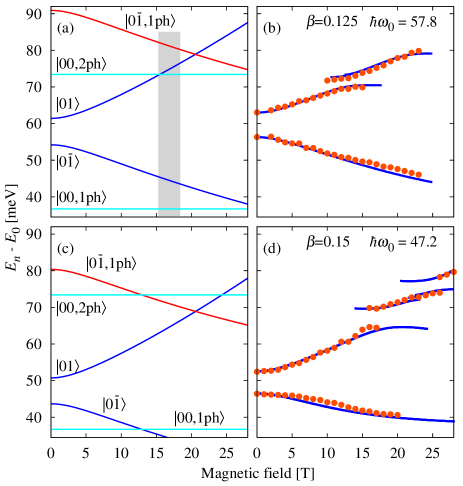
Figure 4: (Color online) (a,c) Dependence of the unperturbed eigenenergies (without electron-phonon coupling) on magnetic field. (b,d) The QD energy spectrum in magnetic field with electron-phonon interaction included. Results obtained with numerical diagonalization of full Hamiltonian (lines) compared with experimental results taken from Refs. hameau99, ; hameau02, (points).

For the present discussion, the intersection between the purely electronic state $|01\rangle$ and a group of 2-phonon states $|00,2\mathrm{ph}\rangle$ is of interest [shaded area in Fig. 4(a)]. In a strong magnetic field, one group of states mediating the interaction ($|0\bar{1},1\mathrm{ph}\rangle$) between 0- and 2-phonon states is much closer to the resonance than at $B=0$. States $|0\bar{1},1\mathrm{ph}\rangle$ are directly coupled to both relevant groups of states. Since the direct interaction is much stronger than indirect one, the resonance between zero-phonon and two-phonon states can be strongly intermixed with 1-phonon states. This is especially the case for QD sizes in between those in Figs. 4(a) and 4(c).

We compare the results of numerical diagonalization with experimental ones hameau99 ; hameau02 obtained for 2 samples differing in QDs sizes. The diagrams presented in Figs. 4(b) and 4(d) consist of several lines that represent transitions to different excited states. The splitting of the $p$-shell states allows one to uniquely determine the anisotropy parameter $\beta$, while the confinement energy $\hbar\omega_{0}$ can be directly read off the spectral position of these $p$-shell states. For low magnetic fields, two lines with an opposite Zeeman shift emerge. At high magnetic fields, the lower lying line strongly interacts with 1-phonon states $|00,1\mathrm{ph}\rangle$, that is, a strong shift towards higher energies is observed. For smaller QDs (and thus higher energy spacing $\hbar\omega_{0}$), for a magnetic field in the range 10-15 T, a clean second-order resonance between $|01\rangle$ and $|00,2\mathrm{ph}\rangle$ states can be observed [Fig. 4(b)]. For a bigger QD [Fig. 4(d)], when the upper line comes close to 1- and 2-phonon states, two resonances appear. One may assume that the first anticrossing in the upper part of this chart is due to the direct interaction between the states $|0\bar{1},1\mathrm{ph}\rangle$ and $|01\rangle$ whereas the second one is a second-order resonance between the states $|00,2\mathrm{ph}\rangle$ and $|01\rangle$. However it must be noted that all these states are relatively close to each other and both, first and second order polarons can be strongly intermixed.

Previous studies hameau99 ; hameau02 ; jacak02a ; jacak03a ; jacak02f suggested that the electron-phonon interaction, measured by the dimensionless Fröhlich constant

$$\alpha_{F}=\frac{e^{2}}{\epsilon_{0}\tilde{\epsilon}}\sqrt{\frac{m^{*}}{2\hbar^{3}\Omega}},$$

needs to be tuned in order to conform with experiment. As a result, the Fröhlich constant, which in principle depends only on material properties, was used as an adjustable parameter. Our present results show that such a treatment is not necessary. As can be seen in Figs. 4(b) and 4(d), both resonance positions and widths are reproduced without the need to enhance the Fröhlich constant after a sufficient number of electron shells and phonon modes has been included in the computational basis. For instance, our numerical solution yields the resonance width of $3.0$ meV in the case shown in Fig. 4(b), which compares quite well with the experimental value of $2.9$ meV. By performing the diagonalization in restricted bases, we have found out that the 3-shell, 3-phonon model is actually minimal in the sense that a further reduction of the basis set leads to incorrect results. In particular, leaving out the $d$-shell states yields a strongly underestimated width of the resonance. On the other hand, not accounting for 3-phonon states moves the resonance to higher magnetic fields and produces nonexistent polaron branches in the resonance area (See Ref. kaczmarkiewicz08, for more details).

$$\begin{array}[]{|c|c|c|}\mathrm{Computational}&\mathrm{Resonance}&\mathrm{Resonance}\\ \mathrm{basis}&\mathrm{width~{}[meV]}&\mathrm{position~{}[T]}\\ \hline\cr\mathrm{Full~{}model}&3.00&13.5\\ \mathrm{3~{}phonons,2~{}shells}&2.10&12.7\\ \mathrm{2~{}phonons,3~{}shells}&2.98&15.2\\ \mathrm{2~{}phonons,2~{}shells}&2.80&14.9\\ \hline\cr\mathrm{Experimental~{}results}&2.9&12-14\\ \end{array}$$

Table 5: Properties of the resonance area for different truncations of the computational basis, compared to experimental results hameau99 .

We have also checked to what extent the numerical results depend on our choice of the $l_{z}/l_{0}$ ratio. For $l_{z}/l_{0}=0.2$, that is, twice larger than used in this paper, only small shift in eigenenergies is observed (approximately $0.1~{}\mathrm{meV}$) and the resonance width decreases to $2.8~{}\mathrm{meV}$, still very close to the experimental result of $2.9~{}\mathrm{meV}$.

V Effective Hamiltonian approach

In the effective Hamiltonian approach, one considers the case of an unperturbed Hamiltonian $H_{0}$ having eigenvalues $E_{i\alpha}$ grouped into well separated manifolds cohen98 . The states can be written in the form $|i\alpha\rangle$, where the Latin indices denote different states within a manifold while Greek indices refer to different manifolds. The corresponding energies of the unperturbed system are $E_{i\alpha}$. Grouping into a manifold means that

$$|E_{i\alpha}-E_{j\alpha}|\ll|E_{i\alpha}-E_{j\beta}|~{}~{}\mathrm{for}~{}\alpha\neq\beta,$$

i.e., energy separation between states from different manifolds, is much larger then energy separations within manifold. Moreover, perturbation-induced coupling between states from different manifolds should be much smaller than the energy separation between these states,

$$|\langle i,\alpha|V|j,\beta\rangle|\ll|E_{i\alpha}-E_{j\beta}|~{}~{}\mathrm{for}~{}\alpha\neq\beta,$$ (5)

where $V$ is the perturbation.

The eigenvalue problem is treated by a quasi-degenerate perturbation theory. The original Hamiltonian $H=H_{0}+V$ is transformed into a new one, $H_{\mathrm{eff}}$, which has no matrix elements between different groups of states (up to the required order of approximation), by means of a unitary transformation $T=e^{iS}$. The matrix elements of the operator $S$ and of $H_{\mathrm{eff}}$ can be found iteratively.

The expression for the second-order effective Hamiltonian has the form cohen98

$$\langle i|H_{\mathrm{eff}}^{\alpha}|j\rangle = E_{i\alpha}\delta_{ij}+\langle i,\alpha|V|j,\alpha\rangle+$$ (6)

$$+\frac{1}{2}\sum_{k,\gamma\neq\alpha}\langle i,\alpha|V|k,\gamma\rangle\langle k,\gamma|V|j,\alpha\rangle$$

$$\times\left[\frac{1}{E_{i\alpha}-E_{k\gamma}}+\frac{1}{E_{j\alpha}-E_{k\gamma}}\right].$$

The first term in Eq. (6) represents the unperturbed energies, the second one accounts for direct couplings within a single manifold, and the last one describes the influence of intermediate states from the different manifolds on the effective Hamiltonian matrix. This last term represents indirect second-order couplings between the states of the manifold of interest which result from the couplings to other manifolds eliminated by the unitary transformation $T$.

The effective Hamiltonian method is a powerful tool for calculations and interpretation of various systems. In the present case of a two-phonon polaron resonance, it is very helpful since in the resonance area a purely electronic state and a group of two-phonon states form a well separated manifold. The method can be used for a description of both magnetopolaron resonances and a size-dependent polaron spectrum, though it is more accurate in the latter case, since the condition for the appropriate relations between energy spacings and coupling strengths [Eq. (5)] is fulfilled in this case with a greater precision.

If one considers the case of the size dependent spectrum (without a magnetic field) the energy difference between states from different manifolds at the point of the resonance is at least $\hbar\Omega=36.7~{}\mathrm{meV}$. On the other hand, if the purely electronic state $|01\rangle$ is brought to resonance with the 2-phonon line $|00,2\mathrm{ph}\rangle$ using a magnetic field, the energy separation is significantly lower. For the cases presented in Figs. 4(a), 4(c), it is approximately 15 and 30% smaller, respectively (assuming that the coupled state $|0\bar{1},1\mathrm{ph}\rangle$ is considered as a member of the manifold). If we take into consideration that the average direct coupling between states from different manifolds is about 3 meV, even 30% reduction in energy separation might impair the applicability condition.

The effective Hamiltonian approach automatically includes the nested coupling polaron structure obreschkow07 , since from the whole spectrum of the states it filters out the ones that are coupled to each other through intermediate states (for a given truncation of the basis).

VI Results: effective Hamiltonian

In the following section, we investigate the second-order resonance using the effective Hamiltonian approach. We consider the case of size dependent spectra as well as a magnetopolaron resonance.

We apply an appropriate treatment to obtain the effective Hamiltonian in both cases, although the latter one might be less applicable in the case of larger QDs (Zeeman tuning brings one-phonon states close to two-phonon line intermixing first and second order resonances and thus breaks the condition for sufficient manifolds separation). Since the energy separation between different states depends on the size of the QD each case should be studied individually.

The effective Hamiltonian approach allows us to gain some information about the second-order polaron structure. Since we choose relevant indirectly coupled states only we can get much insight into the mediated interaction between 0- and 2- phonon states. As the effective Hamiltonian matrix is much smaller than the full Hamiltonian matrix its diagonalization is much faster and interpretation of the spectra is easier. Contributions from different intermediate states can easily be separated and studied. In particular, we investigate the influence of $d$-shell and 3-phonon states on the polaron spectra and on the coupling strengths appearing in the effective Hamiltonian. We show that the quasi-degenerate perturbation theory not only allows one to describe the resonance area in detail, but also explains why both $d$-shell and 3-phonon states have to be used in order to correctly model second-order polarons.

VI.1 Polaron resonance at $B=0$

In this section, we consider the effective Hamiltonian approach to the second-order resonance between states $|01\rangle$ and $|00,2\mathrm{ph}\rangle$ in the absence of a magnetic field. For the sake of simplicity, we assume that the QD is isotropic (it is always possible to introduce anisotropy perturbatively).

Although, for our truncated basis, there are $105$ two-phonon states only $6$ of them couple indirectly (in the second order approximation) to the purely electronic state $|01\rangle$. There is a small number ($12$) of intermediate states which produce nonzero couplings in the effective Hamiltonian. Their contribution is presented (grouped by shell and number of phonons) in Tab. 6. If the numerical values for different shells or different phonon numbers sum up to zero the relevant states are decoupled.

$$\begin{array}[]{|r|ccc|cc|}\hline\cr\vrule\lx@intercol\hfil\mathrm{matrix~{}elements}\hfil\lx@intercol\vrule\lx@intercol&\vrule\lx@intercol\hfil\mathrm{intermediate~{}states}\hfil\lx@intercol\vrule\lx@intercol\\ \cline{2-6}\cr&s&p&d&1\mathrm{ph}&3\mathrm{ph}\\ \hline\cr\langle 01|H_{\mathrm{eff}}|00,A^{2}A^{\bar{1}}\rangle&0&82.8\%&17.2\%&1&0\\ \langle 01|H_{\mathrm{eff}}|00,A^{0}A^{1}\rangle&\lx@intercol\hfil 88.9\%\hfil\lx@intercol&11.1\%&1&0\\ \langle 01|H_{\mathrm{eff}}|00,A^{0}B^{1}\rangle&0&0&100\%&1&0\\ \langle 01|H_{\mathrm{eff}}|00,A^{3}A^{\bar{2}}\rangle&0&0&100\%&1&0\\ \langle 01|H_{\mathrm{eff}}|00,A^{2}B^{\bar{1}}\rangle&0&0&100\%&1&0\\ \langle 01|H_{\mathrm{eff}}|00,B^{0}A^{1}\rangle&50\%&-50\%&0&1&0\\ \langle 00,A^{0}A^{1}|H_{\mathrm{eff}}|00,B^{0}A^{1}\rangle&100\%&0&0&0.5&-0.5\\ \hline\cr\end{array}$$

Table 6: Relative influence of different electronic shells and $n$-phonon states on the effective Hamiltonian couplings in the limit $l_{z}/l_{B}\rightarrow 0$. In the second line, the contributions from the two shells are taken together as they partly cancel each other.

$$\begin{array}[]{|c|r|}\hline\cr H_{\mathrm{eff}}~{}\mathrm{matrix~{}elements}&\lx@intercol\hfil\mathrm{coupling~{}strength}\hfil\lx@intercol\vrule\lx@intercol\\ \hline\cr\langle 01|H_{\mathrm{eff}}|00,A^{2}A^{\bar{1}}\rangle&~{}~{}29\sqrt{3}/(768\sqrt{2\pi})\approx~{}~{}0.0261\\ \langle 01|H_{\mathrm{eff}}|00,A^{0}A^{1}\rangle&~{}~{}13\sqrt{3}/(384\sqrt{2\pi})\approx~{}~{}0.0234\\ \langle 01|H_{\mathrm{eff}}|00,A^{0}B^{1}\rangle&-1/(128\sqrt{\pi})\approx-0.0044\\ \langle 01|H_{\mathrm{eff}}|00,A^{3}A^{\bar{2}}\rangle&-5\sqrt{5}/(256\sqrt{2\pi})\approx-0.0035\\ \langle 01|H_{\mathrm{eff}}|00,A^{2}B^{\bar{1}}\rangle&-1/(256\sqrt{\pi})\approx-0.0022\\ \hline\cr\end{array}$$

Table 7: Indirect coupling strengths in the effective Hamiltonian approach. Coupling strength expressed in units of ${e^{2}}/(2l\varepsilon_{0}\tilde{\varepsilon})=32.7~{}\mathrm{meV}$.

As we can see in Tab. 6, taking the $d$-shell into account not only introduces three additional couplings (rows 3 to 5), but also changes the strength of existing ones (increase of over 17% and 11% in rows 1 and 2, respectively). What is more important, taking $3$-phonon states into account completely decouples the 2-phonon state $|00,B^{0}A^{1}\rangle$ as shown in row 7. Here, $A^{1}$ denotes the phonon mode created by the collective operator $B^{{\dagger}}_{1A}$ [Eq. (3)], etc. Although Tab. 6 is constructed for the limiting case of an infinitely flat QD ($l_{z}\to 0$) and at exact resonance ($\hbar\omega_{0}=2\hbar\Omega$) this decoupling is preserved also for non-flat QDs and is an effect of equal spacing of the electronic eigenenergies in a parabolic confining potential.

The properties of indirect couplings via 1-phonon and 3-phonon states, revealed by the effective Hamiltonian structure, allow one to qualitatively understand why a 3-shell, 3-phonon model is required for correct modelling of the resonant polaron spectrum. Leaving out 3-phonon states leads to a reconstruction of the spectrum (additional lines in the theoretically modelled absorption spectrum are observed, see Fig. 5) since the coupling between states $|00,B^{0}A^{1}\rangle$ and $|00,A^{0}A^{1}\rangle$ in the absence of 3-phonon states is relatively strong. For the case of a flat QD, the coupling strength factor is $0.0288$ which is the strongest coupling comparing to other ones shown in table 7. However, if the 3-phonon states are included this coupling vanishes completely. This shows that a truncation of the computational basis can not only cancel some indirect couplings obreschkow07 but can also lead to the appearance of nonexistent ones. This increases the number of optically active states in the resonance area and affects the spectrum both qualitatively and quantitatively.

Although the cancellation of an indirect interaction between certain 2-phonon states in the presence of 3-phonon states is quite general and similar cancellation of the mediated interaction between other n-phonon states ($n>0$) can be observed it does not necessarily translate to the reduction of the size of the relevant polaronic subspace. In general, such a decoupling is a quantitative effect and may depend not only on the structure of the model, but also on the values of the couplings. For that reason the quasi-degenerate perturbation theory seems to be the right approach, which takes in to account the nested coupling structure obreschkow07 , as well as system dependent quantitative effects.

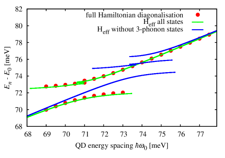
Figure 5: (Color online) Comparison between effective Hamiltonian approach and full Hamiltonian diagonalization. Influence of disregarding 3-phonon states on resonance area also included.

The influence of $d$-shell and 3-phonons states on the diagonal elements of the effective Hamiltonian is found to be less than $0.4\%$ and $2.5\%$ respectively. Coupling with the two-phonon state $|00,A^{2}B^{\bar{1}}\rangle$ is very weak and it is possible to discard it from consideration. Such a reduction of the computational basis does not produce any important effects. The area of the second-order resonant polarons can now be described by a Hamiltonian of dimension 5.

The results obtained with the effective Hamiltonian approach are nearly the same as those obtained with full Hamiltonian diagonalization. The largest shift between eigenenergies found with those two methods in the range of the QD energy spacing presented in Fig. 5 is lower than 0.16 meV.

VI.2 Magnetopolaron resonance

The effective Hamiltonian treatment for a non-zero magnetic field differs slightly from the previous case of zero magnetic field, since the paramagnetic term brings the one-phonon state $|0\bar{1},A^{2}\rangle$ close to the second-order resonance. This additional state couples to the purely electronic state and to certain two-phonon states and, depending on the QD size, can be of major importance. Nevertheless, the resonance area can be precisely described using the quasi-degenerated perturbation theory even in the case of relatively big QDs. When the previously mentioned one-phonon state is too close to the energy of two LO phonons it simply needs to be included as a member of the considered manifold. Since both samples [Figs. 4(b), 4(d)] consist of relatively large QDs this one-phonon state has to be included in the group of relevant states.

$$\begin{array}[]{|c|c|c|}\hline\cr\mathrm{matrix~{}elements}&\lx@intercol\hfil\mathrm{coupling~{}strength}\hfil\lx@intercol\vrule\lx@intercol&d\mathrm{-shell~{}influence}\\ \hline\cr\langle 01|H_{\mathrm{eff}}|00,{A^{2}A^{\bar{1}}}\rangle&~{}~{}1.786&7\%\\ \langle 01|H_{\mathrm{eff}}|00,{A^{0}A^{1}}\rangle&~{}~{}0.627&11\%\\ \langle 01|H_{\mathrm{eff}}|00,{A^{3}A^{\bar{2}}}\rangle&-0.157&100\%\\ \langle 01|H_{\mathrm{eff}}|00,{A^{0}B^{1}}\rangle&-0.143&100\%\\ \langle 01|H_{\mathrm{eff}}|00,{A^{2}B^{\bar{1}}}\rangle&-0.056&100\%\\ \hline\cr\end{array}$$

Table 8: Indirect effective Hamiltonian couplings for case of magnetic field tuning. Values obtained for electron excitation energy $\hbar\omega_{0}=60~{}\mathrm{meV}$ in a magnetic field of $14.1~{}\mathrm{T}$, expressed in meV.

In the construction of the effective Hamiltonian, a set of 6 indirectly coupled states {$|01\rangle$, $|00,A^{0}A^{1}\rangle$, $|00,A^{2}A^{\bar{1}}\rangle$, $|00,A^{3}A^{\bar{2}}\rangle$, $|00,A^{0}B^{1}\rangle$, $|00,A^{2}B^{1}\rangle$} is chosen as a basis (decoupling of certain 2-phonon states, discussed in the previous section, is already taken into account). At this point, we are interested in the strengths of indirect coupling mediated by 1-phonon states, so we temporarily exclude the state $|0\bar{1},A^{2}\rangle$ from the manifold. In this way, the influence of all intermediate 1-phonon states on the second-order resonance can easily be determined. To keep the model reasonably accurate in the absence of this state Tab. 8 is calculated for a QD with a slightly larger characteristic energy $\hbar\omega_{0}$, so that the energy separation between the relevant manifold and the state $|0\bar{1},A^{2}\rangle$ is also larger. Indirect coupling strengths for the resonance condition with the influence of the $d$-shell are presented in Tab. 8. As one can see, in the case of the magnetopolaron spectrum, the presence of the $d$-shell increases the coupling strength significantly (rows 1-2) and couples 3 additional 2-phonon states with the state $|01\rangle$ (rows 3-5). The character of the influence of 3-phonon states is the same as that discussed in the previous subsection.

As we pointed out earlier, in the case of relatively large QDs (when the characteristic energy is lower than 60 meV), additional one-phonon state in the effective Hamiltonian basis needs to be included. If this is done then both methods: diagonalization of the full Hamiltonian and quasi-degenerated perturbation theory approach produce nearly the same results in the resonance area with differences in the obtained eigenenergies and resonance widths smaller than $0.15~{}\mathrm{meV}$ and $0.01~{}\mathrm{meV}$, respectively. Comparison between the results obtained with the effective Hamiltonian approach and the experimental ones are presented in Fig. 6. Good agreement between the theory and experiment can be observed.

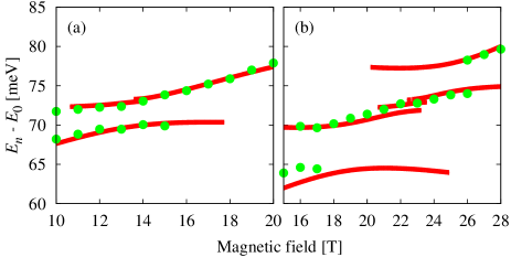
Figure 6: (Color online) Polaron eigenenergies in the resonance area. Dots: experimental results from Refs. hameau99, ; hameau02, , lines: results obtained with the effective Hamiltonian approach. Samples and QD material parameters as in Fig. 4.

VII Conclusions

In this paper, we have theoretically studied the resonant features in the spectrum of an electron confined in a self-assembled QD and interacting with LO phonons. We have focused on the second-order resonance induced by the indirect interaction between the first excited electronic shell ($p$-shell) and the electronic ground state with two LO phonons. We have studied this second order resonant polaron spectrum as a function of the dot size (energy level separation) and external magnetic field. We have also calculated the absorption spectra for an inhomogeneous ensemble of QDs and shown that polaronic feature is clearly manifested in these spectra. Our results, compared to the existing experimental data, show that a properly constructed model is able to quantitatively reproduce the observed polaron resonance without any need for free or adjustable parameters describing the interaction between confined electrons and LO phonons, except for shape and size parameters that can uniquely be extracted from the intraband absorption spectrum.

In order to get more insight into the structure of the polaron spectrum in the resonance area, we have developed an effective Hamiltonian approach based on a quasi-degenerate perturbation theory. We have shown that by tracing the structure of indirect couplings mediated by 1- and 3-phonon states, a very small set of relevant basis states can be identified which span the space of resonant polaron states.

The presented results show that the spectrum of the coupled electron–LO phonon system can be reliably modelled based on the standard theories and computational techniques developed for confined systems. Moreover, they demonstrate that this modeling may be considerably simplified by applying perturbation theory methods, without loosing the accuracy of the results.

Appendix A Influence of 4-phonon states on the ensemble absorption

Since the 4-phonon states do not couple 0- and 2- phonon states, their influence on the 2-phonon feature is negligible. On the other hand, they are important if one considers one-phonon replica of the second-order polarons. We compare here the absorption spectra for two computational bases: one including only states with up to 3 phonons and the other one with additional 4-phonon states (Fig. 7). For the sake of simplicity, results were obtained for the case of an isotropic QD without anharmonicity corrections.

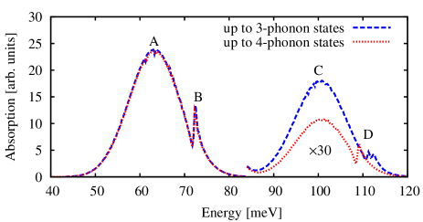
Figure 7: (Color online) Absorption spectra on ensemble of isotropic QDs obtained with and without 4-phonon states. Standard deviation $6~{}\mathrm{meV}$, the mean value $\hbar\overline{\omega_{0}}=62~{}\mathrm{meV}$.

The influence of 4-phonon states on the main absorption peak (A), as well as on 2-phonon resonance (B), is marginal. On the other hand, 4-phonon states are of major importance for one phonon replica features (C,D). Since those features appear as a result of the interaction between 1-phonon and 3-phonon states, 4-phonon states have similar influence on them as 3-phonon states had on the interaction between 0- and 2- phonon states (decoupling of previously strongly coupled states). As a result of introducing additional interacting states, a quantitative change is observed in the intensity of the phonon replica (C) of the main absorption peak. The most important change in the ensemble absorption is related to the phonon replica of the resonant feature (D). If 4-phonon states are omitted this feature is broader and consists of two peaks. On the other hand, if we include 4-phonon states, the replica of the resonant feature consists of one sharp peak, which is shifted towards lower energies. The energy shift is mostly due to presence of directly coupled 4-phonon states with energy $4\hbar\Omega$ which is higher than the energy of the feature D, whereas the change in its shape is related to a reconstruction of the spectrum in the area of the feature D, introduced by those additional states.

References

- (1) U. Bockelmann and G. Bastard, Phys. Rev. B 42, 8947 (1990).
- (2) J. Urayama, T. B. Norris, J. Singh, and P. Bhattacharya, Phys. Rev. Lett. 86, 4930 (2001).
- (3) R. Heitz, H. Born, F. Guffarth, O. Stier, A. Schliwa, A. Hoffmann, and D. Bimberg, Phys. Rev. B 64, 241305(R) (2001).
- (4) S. Hameau, Y. Guldner, O. Verzelen, R. Ferreira, G. Bastard, J. Zeman, A. Lemaître, and J. M. Gerard, Phys. Rev. Lett. 83, 4152 (1999).
- (5) O. Verzelen, R. Ferreira, and G. Bastard, Phys. Rev. Lett. 88, 146803 (2002).
- (6) S. Hameau, J. N. Isaia, Y. Guldner, E. Deleporte, O. Verzelen, R. Ferreira, G. Bastard, J. Zeman, and J. M. Gérard, Phys. Rev. B 65, 085316 (2002).
- (7) O. Verzelen, R. Ferreira, and G. Bastard, Phys. Rev. B 62, R4809 (2000).
- (8) L. Jacak, J. Krasnyj, D. Jacak, and P. Machnikowski, Phys. Rev. B 65, 113305 (2002).
- (9) T. Grange, R. Ferreira, and G. Bastard, Phys. Rev. B 76, 241304(R) (2007).
- (10) R. Heitz, M. Veit, N. N. Ledentsov, A. Hoffmann, D. Bimberg, V. M. Ustinov, P. S. Kop’ev, and Z. I. Alferov, Phys. Rev. B 56, 10435 (1997).
- (11) I. V. Ignatiev, I. E. Kozin, V. G. Davydov, S. V. Nair, J.-S. Lee, H.-W. Ren, S. Sugou, and Y. Masumoto, Phys. Rev. B 63, 075316 (2001).
- (12) E. A. Zibik, L. R. Wilson, R. P. Green, G. Bastard, R. Ferreira, P. J. Phillips, D. A. Carder, J.-P. R. Wells, J. W. Cockburn, M. S. Skolnick, M. J. Steer, and M. Hopkinson, Phys. Rev. B 70, 161305(R) (2004).
- (13) R. Haupt and L. Wendler, Physica B 184, 394 (1993).
- (14) L. Wendler, A. V. Chaplik, R. Haupt, and O. Hipólito, J. Phys.: Condens. Matter 5, 8031 (1993).
- (15) L. Jacak, P. Machnikowski, J. Krasnyj, and P. Zoller, Eur. Phys. J. D 22, 319 (2003).
- (16) D. Obreschkow, F. Michelini, S. Dalessi, E. Kapon, and M.-A. Dupertuis, Phys. Rev. B 76, 035329 (2007).
- (17) T. Stauber, R. Zimmermann, and H. Castella, Phys. Rev. B 62, 7336 (2000).
- (18) L. Jacak, J. Krasnyj, and W. Jacak, Phys. Lett. A 304, 168 (2002).
- (19) L. Jacak, P. Hawrylak, and A. Wójs, Quantum Dots (Springer Verlag, Berlin, 1998).
- (20) L. Jacak, J. Krasnyj, D. Jacak, and P. Machnikowski, Phys. Rev. B 67, 035303 (2003).
- (21) P. Kaczmarkiewicz and P. Machnikowski, Acta Phys. Pol. A 114, 1139 (2008).
- (22) C. Cohen-Tannoudji, J. Dupont-Roc, and G. Grynberg, Atom-Photon Interactions (Wiley-Interscience, New York, 1998).