Perpetuities with thin tails, revisited

Abstract.

We consider the tail behavior of random variables $R$ which are solutions of the distributional equation $R\stackrel{{\scriptstyle d}}{{=}}Q+MR$, where $(Q,M)$ is independent of $R$ and $|M|\leq 1$. Goldie and Grübel showed that the tails of $R$ are no heavier than exponential and that if $Q$ is bounded and $M$ resembles near 1 the uniform distribution, then the tails of $R$ are Poissonian. In this paper we further investigate the connection between the tails of $R$ and the behavior of $M$ near 1. We focus on the special case when $Q$ is constant and $M$ is non–negative.

1. Introduction

In this note we consider a random variable $R$ given by the solution of the stochastic equation

(1.1) $$R\stackrel{{\scriptstyle d}}{{=}}Q+MR,$$

where $(Q,M)$ are independent of $R$ on the right-hand side. Under suitable assumptions on $(Q,M)$ one can think of $R$ as a limit in distribution of the following iterative scheme

(1.2) $$R_{n}=Q_{n}+M_{n}R_{n-1},\quad n\geq 1$$

where $R_{0}$ is arbitrary and $(Q_{n},M_{n})$, $n\geq 1$, are i.i.d. copies of $(Q,M)$, and $(Q_{n},M_{n})$ is independent of $R_{n-1}$. Writing out the above recurrence and renumbering the random variables $(Q_{n},M_{n})$ we see that $R$ may also be defined by

(1.3) $$R\stackrel{{\scriptstyle d}}{{=}}\sum_{j=1}^{\infty}Q_{j}\prod_{k=1}^{j-1}M_{k},$$

provided that the series above converges in distribution. Sufficient conditions for the almost sure convergence are known and have been given by Kesten [13] who also considered a multidimensional case when $M$ is a matrix and $Q$ a vector. For a nice detailed discussion of a one dimensional case we refer to the paper by Vervaat [19]; we only mention briefly here that ${\mathbb{E}}\log^{+}|Q|<\infty$ and ${\mathbb{E}}\log|M|<0$ suffice for the almost sure convergence of the series in (1.3)

In the form (1.3) $R$ has been studied in insurance mathematics under the name perpetuity. Since schemes like (1.2) are ubiquitous in many areas of applied mathematics, the properties of $R$ have attracted a considerable interest. We refer to [5, 6, 7, 8, 13, 16, 19] and references therein for more information and sample of applications. For examples of more recent work on perpetuities and their applications see [1, 2, 11, 14]. A few additional situations in which perpetuities arise will be mentioned below.

The main focus of research is the tail behavior of $R$. Kesten [13] showed that if ${\mathbb{P}}(|M|>1)>0$ then $R$ is always heavy–tailed. More precisely, he showed that if there exists a $\kappa$ such that ${\mathbb{E}}|M|^{\kappa}\log^{+}|M|<\infty$, ${\mathbb{E}}|Q|^{\kappa}<\infty$, and ${\mathbb{E}}|M|^{\kappa}=1$ then for some constant $C$

$${\mathbb{P}}(|R|\geq x)\sim Cx^{-\kappa},\quad\mbox{as}\quad x\to\infty.$$

Here, and throughout the paper the symbol $f(x)\sim g(x)$ means that the ratio goes to 1 as $x\to\infty$. His result was rediscovered, reproved, and extended by several authors (see [7, 9, 10]). In the complementary case, ${\mathbb{P}}(|M|\leq 1)$ the picture is much less clear. The main work we are aware of is that of Goldie and Grübel [8] who showed that in that case, the tails are never heavier than exponential and that if $M$ behaves near 1 as a uniform random variable then the tails have Poissonian decay. In their arguments Goldie and Grübel relied on inductive arguments applied to (1.2).

The main purpose of this note is to use systematically their approach to obtain additional information on the links between the behavior of $M$ near 1 and the tail behavior of $R$. Following Goldie and Grübel (and also customs in large deviation theory) we will be interested in the asymptotics of the logarithm of the tail probability, i.e. $\ln{\mathbb{P}}(|R|\geq x)$ as $x\to\infty.$ Since we are mainly interested in establishing the links between $M$ and $R$, we will often make additional, but common, assumptions when necessary. For example, we generally assume that $Q$ and $M$ are independent or even that $Q\equiv q$ is non–random. The independence assumption is typically needed only for the lower bounds on the log of the tail probability, the upper bounds are usually obtainable without it. Once the independence of $Q$ and $M$ is assumed the restriction that $Q$ is degenerate does not seem to be a major restriction, but makes some of the arguments more transparent. It is rather the assumption that $Q$ is bounded, which seems to play the more important role. Similarly, we will assume that $M$ and $q$ are non–negative. How the non–negative case differs from the general is relatively well understood (see e.g. arguments in [8, Theorem 2.1, Theorem 3.1, Lemma 5.3]) to see how arguments for non–negative case can be extended to more general situations.

We would like to mention an interesting connection of perpetuities with a subclass of infinitely divisible laws, namely, as was shown by Jurek [12] all self–decomposable random variables (we refer to [12] for the definition) can be represented as perpetuities $R$ given by (1.1) with $0\leq M\leq 1$. As a matter of fact, much more is shown in [12], namely, if $R$ is self–decomposable then for every random variable $0\leq M\leq 1$ there exists a random variable $Q$ (typically not bounded) such that (1.1) holds with $(Q,M)$ independent of $R$ on the right–hand side. This curious result seems to be of little help as far as general theory of perpetuities goes. In fact, one can take $M$ to be any constant $M=m\in(0,1)$ and equally well represent a self–decomposable random variable as a series of weighted i.i.d. random variables, with weights forming a geometric progression. Nonetheless, we mention that building on an earlier work of Thorin [18, 17], Bondesson [3] proved a general result which implies, in particular, that all gamma, inverse gamma, Pareto, log–normal, and Weilbull distributions are self–decomposable. Some of these results were obtained earlier by other authors and we refer to Bondesson [3, Section 5] for credits and more examples.

2. General outline

To begin the discussion, assume that $|M|\leq 1$. Trivially, if $|Q|\leq q$ and $|M|$ is concentrated on a proper subinterval $(0,1-\delta)$, $\delta>0$ of $(0,1)$ then the perpetuity $R$ is a random variable whose absolute value is bounded by $q/\delta$ and thus has a trivial tail in the sense that ${\mathbb{P}}(|R|\geq x)=0$ for $x>q/\delta$. On the other hand if $M$ is not bounded away from 1 then we have the following observation due to Goldie and Grübel:

Proposition 1.

For $\delta\in(0,1)$ let $p_{\delta}:={\mathbb{P}}(1-\delta\leq M\leq 1)$. Then for every such $\delta$ and for all $y>0$ we have

(2.1) $${\mathbb{P}}(R\geq\frac{q}{\delta}(1-(1-\delta)^{y}))\geq p_{\delta}^{y}.$$

In particular, if for $c\in(0,1)$ and $x>q$ we set

$$\delta=\frac{cq}{x}\quad\mbox{and}\quad y=\frac{\ln(1-c)}{\ln(1-cq/x)},$$

then we get that

(2.2) $${\mathbb{P}}(R\geq x)\geq\left(p_{\frac{cq}{x}}\right)^{\frac{\ln(1-c)}{\ln(1-cq/x)}}=\exp\left(\frac{\ln(1-c)}{\ln(1-cq/x)}\ln(p_{\frac{cq}{x}})\right).$$

Proof: This was observed by Goldie–Grübel: For a given $\delta>0$ we let

$$\tau=\tau_{\delta}=\inf\{n\geq 1:\ M_{n}<1-\delta\}.$$

Then by non–negativity and (1.3), on $\{\tau\geq n\}$ we have

$$R\geq\sum_{k=1}^{n}q(1-\delta)^{k-1}=\frac{q}{\delta}\left(1-(1-\delta)^{n}\right).$$

Therefore, for all $n\geq 1$,

$${\mathbb{P}}(R\geq\frac{q}{\delta}(1-(1-\delta)^{n}))\geq{\mathbb{P}}(M_{k}\geq 1-\delta,\ 1\leq k<n)=p_{\delta}^{n-1}.$$

Hence,

$${\mathbb{P}}(R\geq\frac{q}{\delta}(1-(1-\delta)^{y}))\geq p_{\delta}^{y},\quad\mbox{for all $y>0$}$$

which proves (2.1); (2.2) follows by a simple calculation. $\Box$

It is clear from the above proposition that if $p_{\delta}$ is strictly positive for every $\delta>0$ then the perpetuity $R$ has non-trivial tails. It is then the behavior of $M$ near 1 that determines the nature of the tails of $R$. It appears that essentials of such a behavior are shared by a class of equivalent distributions in the following sense.

Let $\mu$ and $\nu$ be probability distributions on $[0,1]$. For any $\delta\in(0,1)$ we denote $\mu_{\delta}=\mu((1-\delta,1])$ and $\nu_{\delta}=\nu((1-\delta,1])$ We say that the distributions $\mu$ and $\nu$ are equivalent at 1 if

$$\exists\ \varepsilon>0\quad\mbox{and}\quad 0<d<D<\infty\quad\mbox{such that}$$

(2.3) $$\forall\delta\in(0,\varepsilon]:\quad d\leq\frac{\mu_{\delta}}{\nu_{\delta}}\leq D\;.$$

As we mentioned earlier, our goal here is to shed some additional light on the relationship between the behavior of the distribution of $M$ in the left neighborhood of 1 and the tails of $R$. To accomplish that we will develop in a systematic way the approach of Goldie and Grübel. For the upper bound this approach relies on iteration of (1.2) to get a uniform upper bound on the moment generating function of $R_{n}$ for all $n\geq 1$ and then use exponentiation and Markov inequality to translate this bound into bounds on the tails. We will develop this in the next section, but to give a flavor of this argument we provide the following illustration: Consider (1.1) and assume that $Q$, $M$, and $R$ on the right-hand side of (1.1) are independent (that is of course stronger than the usual assumption that $(Q,M)$ are independent of $R$). Also, assume that $0\leq M\leq 1$ and that $m:={\mathbb{E}}M<1$. To get an upper bound on the moment generating function ${\mathbb{E}}e^{zR}$ of $R$, the principle of what Goldie-Grübel did is the following: for $n\geq 1$ we have

$${\mathbb{E}}e^{zR_{n}}={\mathbb{E}}e^{z(Q_{n}+M_{n}R_{n-1})}={\mathbb{E}}e^{zQ}{\mathbb{E}}e^{zMR_{n-1}}\leq{\mathbb{E}}e^{zQ}\left\{1+m{\mathbb{E}}(e^{zR_{n-1}}-1)\right\},$$

where in the last step we use the fact that for $s>0$

(2.4) $${\mathbb{E}}e^{sM}\leq{\mathbb{E}}e^{s\rm Bin(1,m)}=1+m(e^{s}-1).$$

To set up an induction we seek a function $A(z)$ such that

• $Ee^{zR_{n-1}}\leq A(z)$, and

• ${\mathbb{E}}e^{zQ}\left\{1+m(A(z)-1)\right\}\leq A(z)$.

Solving (ii) gives

$$B(z):=\frac{(1-m){\mathbb{E}}e^{zQ}}{1-m{\mathbb{E}}e^{zQ}}\leq A(z),$$

for $z$ such that $m{\mathbb{E}}e^{zQ}<1$. Now, $B(z)$ is recognized as the moment generating function of $\sum_{k=1}^{N}Q_{k}$ where $N\stackrel{{\scriptstyle d}}{{=}}\rm Geom(1-m)$ and is independent of the sequence $Q_{k}$, $k\geq 1$. So if we start with any $R_{0}$ for which (i) holds with $B(z)$ in place of $A(z)$ then the induction goes through and, under a reasonably weak assumptions on $Q$, we get an exponential upper bound on the tail of $R$. In particular if we take $Q\equiv 1$ and $M\stackrel{{\scriptstyle d}}{{=}}\rm Bin(1,m)$ then $R$ has moment generating function bounded by that of a geometric random variable and hence sub-exponential tails as was already shown by Goldie and Grübel.

We mention briefly that the sums described by $B(z)$ are yet another example of perpetuities. Sums like these are of interest in renewal theory and risk assessment, for example. They have been studied before, for instance in [4, 20], under the name geometric convolutions and geometric random sums, respectively. We refer the interested reader there for more information and further references.

As for the lower bound, the best that is available at this point is argument based on Proposition 1. Interestingly, this proposition provides a surprisingly good lower bound. By this we mean the fact that if the upper bound obtained by the above method is constructed carefully so as to be relatively tight, then one can usually obtain a lower bound of a similar strength from Proposition 1. This will be seen in several situations below. It is thus important to understand how to construct a tight upper bound. Although we do not have a general result to that effect, in the last section we will provide an argument in a particular example that provides a heuristic which should work well in other cases.

The rest of the paper is organized as follows, in the next section we will discuss an upper bound and in particular, we will state an inequality (see (3.6) below) that is crucial for the inductive argument. In subsequent sections we will illustrate this with several examples. Those include beta$(\alpha,\beta)$ densities, and what (for the lack of a better name) we call the generalized beta$(1,\beta)$ densities. The reason for considering beta distributions is that one might reasonably hope that they provide a natural parametrization of a behavior of $M$ near 1, which could be translated to the tail behavior of $R$. This, however, is not the case, since as we will show all beta distributions lead to the same, namely Poissonian, behavior. It turns out that a much more rapid than power–type variability of $M$ at 1 is needed to observe a different tail behavior of $R$. We will then construct densities for which the logarithm of the tail probability will have power behavior $-x^{r}$, for $1<r<\infty$. In the last section we will discuss one more example mainly to illustrate a techinque of constructing $M$ that would give a particular tail behavior of $R$ in other situations.

3. Upper bounds

We begin with the following well–known fact.

Proposition 2.

Suppose that

(3.1) $${\mathbb{E}}e^{zX}\leq\exp(B\Phi(z)),$$

for some function $\Phi:\ [0,\infty)\to[0,\infty)$, $B>0$ and all $z>0$. Then

(3.2) $${\mathbb{P}}(X\geq x)\leq e^{-\Phi^{*}(x)},$$

where $\Phi^{*}=\Phi_{B}^{*}$ is defined by

(3.3) $$\Phi^{*}(x)=\sup\{zx-B\Phi(z):\ z>0\}.$$

Note that if $\Phi$ is an Orlicz function (a convex, continuous, non–decreasing function, such that $\Phi(0)=0$ and $\Phi(t)\to\infty$ as $t\to\infty$) then $\Phi^{*}$ is just a complementary function to $\Phi$.

Proof: This is well–known; by the usual exponentiation and Markov’s inequality we have

$${\mathbb{P}}(X\geq x)={\mathbb{P}}(e^{zX}\geq e^{zx})\leq e^{-zx}{\mathbb{E}}e^{zX}\leq e^{-zx}e^{B\Phi(z)}=e^{-(zx-B\Phi(z))}.$$

Since the right–hand side may be minimized over $z$ we obtain (3.2) as required. $\Box$

One can obtain a bound on the moment generating function of $R$ using the fact that it is a limit in distribution of the iterative procedure (1.2) and verifying (3.1) for every $R_{n}$. In the case $Q_{n}\equiv q$ (1.2) takes the form

(3.4) $$R_{n}\stackrel{{\scriptstyle d}}{{=}}q+M_{n}R_{n-1},$$

where $M_{n}$ is a copy of $M$ independent of $R_{n-1}$. To argue inductively, suppose that for some $B>0$

(3.5) $${\mathbb{E}}e^{zR_{n-1}}\leq\exp(B\Phi(z)),\quad z>0.$$

Then by (3.4) and (3.5) applied conditionally on $M_{n}$ we have

$${\mathbb{E}}e^{zR_{n}}=e^{qz}{\mathbb{E}}e^{zM_{n}R_{n-1}}\leq e^{qz}{\mathbb{E}}e^{B\Phi(zM_{n})}.$$

The inductive step will be complete once we show that

$$e^{qz}{\mathbb{E}}e^{B\Phi(zM)}\leq e^{B\Phi(z)}.$$

In terms of the distribution $\mu$ of $M$, the above inequality reads

(3.6) $$e^{qz}\int_{0}^{1}e^{B\Phi(zt)}\mu(dt)\leq e^{B\Phi(z)}.$$

Once this inequality is established, the induction is complete as one can start with arbitrary random variable $R_{0}$, so in particular we can ensure that (3.5) holds for $R_{0}$. The above inequality is crucial for establishing the upper bound.

We will be interested in the tail bounds for large values of $x$. We assume that $\Phi$ is non-degenerate ($\Phi(t)\neq 0$ for $t\neq 0$) and satisfies $\Phi(t)/t\to\infty$ as $t\to\infty$ (i.e. $\Phi$ is an $N$–function in the language of [15]). Then $\Phi^{*}$ has the same properties and it follows directly from the definition (3.3) that as $x\to\infty$ the supremum in (3.3) is attained at $z\to\infty$. This means that it suffices that (3.1) and thus (3.6) hold only for large values of $z$. Thus, we have the following consequence of the above discussion:

Proposition 3.

Let $R$ be given by (1.1) with $Q\equiv q$. Suppose that there exist $B>0$ and $z_{0}$ such that (3.6) is satisfied for the distribution of $M$ for all $z\geq z_{0}$. Then

(3.7) $$\limsup_{x\to\infty}\frac{\ln{\mathbb{P}}(R\geq x)}{\Phi^{*}_{B}(x)}\leq-1.$$

4. Beta distributions

As earlier we will denote by $\mu$ the distribution of $M$. Goldie–Grübel [8, Theorem 3.1] showed that if $Q$ is bounded and $\mu$ and the uniform distribution on $[0,1]$ are equivalent at 1 in the sense of (2.3) then the resulting perpetuity has Poissonian tails, that is

$$\lim_{x\to\infty}\frac{\ln{\mathbb{P}}(R\geq x)}{x\ln x}=-\frac{1}{q}.$$

Note that uniform and beta $\beta(\alpha,1)$ distributions are equivalent at 1. One might reasonably hope that considering other values of the second parameter of the beta distribution might lead to a different tail behavior of $R$ but this is not the case. As we show below any $M$ whose distribution is equivalent at 1 to a measure with polynomial density at 1 leads to the Poissonian tails of $R$.

Theorem 4.

Let the distribution of $M$ and the $\mbox{beta}({\alpha},\beta)$ distribution be equivalent at 1. Assume that $Q\equiv q>0$. Then

$$\lim_{x\to\infty}\frac{\ln{\mathbb{P}}(R\geq x)}{x\ln x}=-\frac{\beta}{q}.$$

Proof: Note that all beta distributions with the same $\beta$ parameter and different ${\alpha}$ parameters are equivalent in the sense of (2.3). Consequently, we assume for convenience that ${\alpha}=1$ so that we consider the beta distribution with the density

$$f(t)=\beta(1-t)^{\beta-1},\quad 0<t<1\;,$$

which is equivalent to the distribution of $M$ at 1.

We show that regardless of the value of $\beta>0$ the tails of the resulting perpetuities are Poissonian. To get an upper bound we verify that (3.6) holds with $\Phi(z)=e^{bz}$ for a suitable constant $b$ and some $B>0$. Once this is done, it follows from the discussion in the previous section that

$$\ln{\mathbb{P}}(R\geq x)\leq-\frac{x}{b}\ln\left(\frac{x}{Bbe}\right)=-\frac{1}{b}x\left(\ln x-\ln(Bbe)\right).$$

which implies that

(4.1) $$\limsup_{x\to\infty}\frac{\ln{\mathbb{P}}(R\geq x)}{x\ln x}\leq-\frac{1}{b}.$$

Thus we are to show that for sufficiently large $z>0$

(4.2) $$e^{qz}\int_{0}^{1}\exp(Be^{bzt})\mu(dt)\leq\exp(Be^{bz}),$$

for some positive constant $B$ and $b=q/\beta$. To that end take an $\varepsilon$ for which (2.3) holds with $\nu$ being a $\mbox{beta}(1,\beta)$ distribution. Assume a $t_{0}$ is chosen so that $t_{0}>1-\varepsilon$. We split the integral on the left–hand side as

$$e^{qz}\int_{0}^{t_{0}}\exp(Be^{bzt})\mu(dt)+e^{qz}\int_{t_{0}}^{1}\exp(Be^{bzt})\mu(dt).$$

The second term, through (2.3) is bounded by

$$De^{qz}\exp(Be^{bz})\beta\int_{t_{0}}^{1}(1-t)^{\beta-1}dt=De^{qz}\exp(Be^{bz})(1-t_{0})^{\beta}.$$

Pick $t_{0}=t_{0}(z)>1-\varepsilon$ so that

(4.3) $$\rho:=De^{qz}(1-t_{0})^{\beta}<1.$$

In order to establish (4.2) we are to show that

$$e^{qz}\int_{0}^{t_{0}}\exp(Be^{bzt})\mu(dt)\leq(1-\rho)\exp(Be^{bz}).$$

It follows from (4.3) that

$$t_{0}=1-e^{-qz/\beta}(\rho/D)^{1/\beta},$$

and thus for sufficiently large $z$ we have that $t_{0}>1-\varepsilon$. Hence, the left–hand side above, by (2.3) again, is bounded by

$$e^{qz}\exp(Be^{bzt_{0}})\mu(0,t_{0})\leq e^{qz}\exp(Be^{bzt_{0}})\left(1-\frac{d}{D}\rho e^{-qz}\right),$$

and we want this to be less or equal than $(1-\rho)\exp(Be^{bz})$. Divide both sides by $\exp(Be^{qz})$ so that the inequality to be proved reads

$$e^{qz}\exp\left(Be^{bzt_{0}}-Be^{bz}\right)\left(1-\frac{d}{D}\rho e^{-qz}\right)\leq 1-\rho.$$

We drop the factor $1-\frac{d}{D}\rho e^{-qz}$ on the left and look at the exponent. It is

$$qz+Be^{bz(1-e^{-qz/\beta}(\rho/D)^{1/\beta})}-Be^{bz}=qz+Be^{bz}\left(e^{-bze^{-qz/\beta}(\rho/D)^{1/\beta}}-1\right).$$

Set $b:=q/\beta$. Since $\rho/D<1$ we have $bze^{-qz/\beta}(\rho/D)^{1/\beta}=bze^{-bz}(\rho/D)^{1/\beta}<bze^{-bz}\leq e^{-1}<\ln 2$. Since $e^{-u}-1\leq-u/2$ for $0<u<\ln 2$ we see that the expression above is bounded by

$$qz-Bbz\rho^{1/\beta}e^{bz}e^{-bz}/2=qz\left(1-\frac{B\rho^{1/\beta}}{2\beta}\right),$$

and it is clear that

$$e^{qz}\exp\left(Be^{bzt_{0}}-Be^{bz}\right)\leq\exp\left(qz(1-\frac{B\rho^{1/\beta}}{2\beta})\right),$$

can be made arbitrarily small by increasing $B$ if necessary. In particular, we can ensure that it is less than $1-\rho$ for all $z$ not too close to 0. Thus, (4.1) is proved with $b=q/\beta$.

To get the matching lower bound note that using again instead of $M$ the equivalent law ${\rm beta}(1,\beta)$ with the cdf $F(t)=1-(1-t)^{\beta}$ we have

$$\nu_{\delta}=1-F(1-\delta)=\delta^{\beta}.$$

Thus, by (2.3)

$${\mathbb{P}}(R\geq x) \geq \left(d\frac{cq}{x}\right)^{\beta\frac{\ln(1-c)}{\ln(1-cq/x)}}=\exp\left(-\beta\frac{\ln(1-c)}{\ln(1-cq/x)}(\ln x-\ln(dcq))\right)$$

$$= \exp\left(\beta\frac{\ln(1-c)}{cq}(x\ln x)(1+o(1))\right).$$

Hence, by letting $c\to 0_{+}$ we get that

$$\liminf_{x\to\infty}\frac{\ln{\mathbb{P}}(R\geq x)}{x\ln x}\geq-\frac{\beta}{q}.$$

$\Box$

5. Generalized beta$(1,\beta)$ distributions

In this section we consider $M$’s whose distributions are equivalent in the sense (2.3) to distribution function given by

(5.1) $$F(s)=F_{\beta,\eta}(s)=1-e^{-\beta(-\ln(1-s))^{\eta}},\quad 0<s<1,\quad\beta,\eta>0.$$

It is elementary to verify that $F_{\beta,\eta}$ is indeed a distribution function which is strictly increasing on $(0,1)$. Furthermore, $F_{\beta,1}$ is the distribution of a $\mbox{beta}(1,\beta)$ random variable discussed in the previous section. The family $F_{\beta,\eta}$ has the following property

$$F^{-1}_{\beta,\eta}=F_{\beta^{-1/\eta},\eta^{-1}},$$

as can be easily verified by a direct calculation. Pictures of a few such distributions with various parameters are given in Figures 1–2.

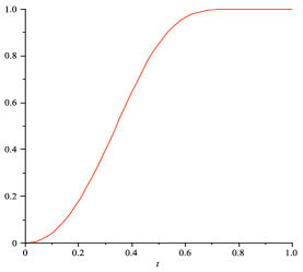
a b

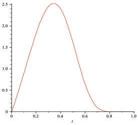
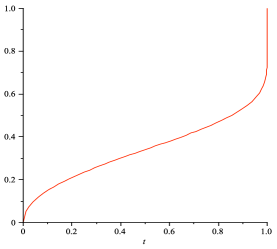
c d

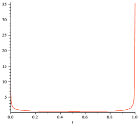
Figure 1. (a) The distribution $F_{4,2}$,  (b) its density,  (c) its inverse $F_{0.5,0.5}$,  and (d) its density.

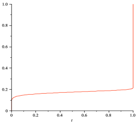
a b

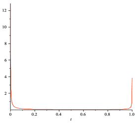
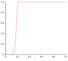
c d

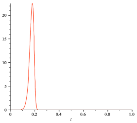
Figure 2. (a) The distribution $F_{0.2,0.1}$,  (b) its density,  (c) its inverse $F_{5^{10},10}$,   and (d) its density.

For $R$ generated with $M$’s with distributions equivalent to the above distribution function the following extension of Theorem 4 holds

Theorem 5.

Let $(R_{n})$ be given by (3.4) where $q>0$ and $M$ has the distribution equivalent to the distribution function (5.1) for some $\beta,\eta>0$. Let $R$ be a limit in distribution of $(R_{n})$. Then

$$\lim_{x\to\infty}\frac{\ln{\mathbb{P}}(R\geq x)}{x(\ln x)^{\eta}}=-\frac{\beta}{q}.$$

Proof: For the upper bound we will show that $R$ satisfies Proposition 3 with $\Phi(z)=\exp(bz^{1/\eta})$ for $b$’s in a certain range. For this $\Phi$ we have

$$\Phi^{*}(x)\geq x\left(\left(\frac{\ln x}{b}\right)^{\eta}-B\right)$$

which can be seen by using $\Phi_{B}^{*}(x)\geq xz_{0}-Be^{bz_{0}^{1/\eta}}$ with $z_{0}=b^{-\eta}(\ln x)^{\eta}$. It follows that

(5.2) $$\limsup_{x\to\infty}\frac{\ln{\mathbb{P}}(R\geq x)}{x(\ln x)^{\eta}}\leq-\frac{1}{b^{\eta}}.$$

To verify (3.6) we will use the same argument as before; with $\Phi(z)=\exp(bz^{1/\eta})$ it becomes

$$e^{qz}\int_{0}^{1}\exp(Be^{b(zt)^{1/\eta}})\mu(dt)\leq\exp(Be^{bz^{1/\eta}}),$$

where $\mu$ is the distribution of the rv $M$ and $b$ and $B$ are positive constants. Splitting the left–hand side, with $t_{0}>1-\varepsilon$ as before we have

$$\beta e^{qz}\int_{0}^{t_{0}}\exp(Be^{b(zt)^{1/\eta}})\mu(dt)+e^{qz}\int_{t_{0}}^{1}\exp(Be^{b(zt)^{1/\eta}})\mu(dt).$$

By (2.3) the second term is bounded by

$$De^{qz}\exp\left(Be^{bz^{1/\eta}}\right)(1-F_{\beta,\eta}(t_{0}))\;.$$

Choose $t_{0}$ so that $\rho:=De^{qz}(1-F(t_{0}))<1$. Then

$$t_{0} = F_{\beta,\eta}^{-1}(1-\rho e^{-qz}/D)$$

$$= F_{\beta^{-1/\eta},\eta^{-1}}(1-\rho e^{-qz}/D)=1-\exp\left(-\beta^{-1/\eta}(-\ln(\rho e^{-qz}/D))^{1/\eta}\right)$$

$$= 1-\exp\left(-\left(\frac{qz}{\beta}\right)^{1/\eta}\left(1-\frac{\ln(\rho/D)}{qz}\right)^{1/\eta}\right),$$

and for $z$ sufficiently large it follows that $t_{0}>1-\varepsilon$. Now we are to prove that

$$e^{qz}\exp\left(Be^{bz^{1/\eta}t_{0}^{1/\eta}}\right)\mu(0,t_{0})\leq(1-\rho)\exp\left(Be^{bz^{1/\eta}}\right)\;.$$

By the first part of (2.3), it is enough to show that

(5.3) $$e^{qz}\exp\left(Be^{bz^{1/\eta}}\left(e^{-bz^{1/\eta}(1-t_{0}^{1/\eta})}-1\right)\right)\left(1-\frac{d\rho}{D}e^{-qz-Be^{bz^{1/\eta}}}\right)\leq 1-\rho.$$

We drop the last factor on the left–hand side as it is less that 1. For $t_{0}$ as above $z^{1/\eta}(1-t_{0}^{1/\eta})$ is close to 0 for $z$ sufficiently large, so that using approximations $e^{-x}-1\sim-x$ and then $1-(1-x)^{\eta}\sim x/\eta$, both valid for $x$ close to 0 we see that the exponent on the left–hand side for $z$ sufficiently large, is

$$qz+Be^{bz^{1/\eta}}\left(e^{-bz^{1/\eta}(1-t_{0}^{1/\eta})}-1\right)\sim qz-Bbz^{1/\eta}e^{bz^{1/\eta}}(1-t_{0}^{1/\eta})$$

$$\quad\sim qz-\frac{Bb}{\eta}z^{1/\eta}\exp\left(z^{1/\eta}\left\{b-\left(\frac{q}{\beta}\right)^{1/\eta}\left(1-\frac{\ln\rho/D}{qz}\right)^{1/\eta}\right\}\right)$$

$$\quad\sim qz-\frac{Bb}{\eta}z^{1/\eta}\exp\left(z^{1/\eta}\left\{b-(q/\beta)^{1/\eta}\right\}\right).$$

For $b>(q/\beta)^{1/\eta}$ the second term grows faster than linearly in $z$, so that as long as $z$ is not too close to 0 it can be made arbitrarily larger than $qz$. Thus, (5.3) follows. Furthermore, letting $b\to(q/\beta)^{1/\eta}_{+}$ in (5.2) we obtain that

(5.4) $$\limsup_{x\to\infty}\frac{\ln{\mathbb{P}}(R\geq x)}{x(\ln x)^{\eta}}\leq-\frac{\beta}{q}.$$

To get a lower bound note that, using instead of the distribution of $M$ the equivalent cdf $F_{\beta,\eta}$, on noting that

$$1-F_{\beta,\eta}(1-cq/x)=\exp\left(-\beta\left(-\ln(cq/x)\right)^{\eta}\right)=\exp\left(-\beta(\ln x-\ln(cq))^{\eta}\right)$$

we get for large $x$

$${\mathbb{P}}(R\geq x) \geq \left(d(1-F_{\beta,\eta}(1-cq/x))\right)^{\frac{\ln(1-c)}{\ln(1-cq/x)}}$$

$$= \exp\left(-\frac{\ln(1-c)}{\ln(1-cq/x)}\beta[(\ln x-\ln(cq))^{\eta}+\ln(d)]\right)$$

$$= \exp\left(\frac{\beta\ln(1-c)}{cq}x(\ln x)^{\eta}(1-o(1))\right).$$

Upon letting $c\to 0_{+}$ it implies that

$$\liminf_{x\to\infty}\frac{\ln{\mathbb{P}}(R\geq x)}{x(\ln x)^{\eta}}\geq-\frac{\beta}{q}\;.$$

Combining this with (5.4) completes the proof. $\Box$

6. Weilbull–like tails

In this section we explicitly construct $M$’s that will lead to a rather different tail behavior of $R$ than discussed in the previous sections. As we will see a much more rapid variability of $M$ near 1 is needed to obtain a lighter tail behavior of $R$. More specifically, we prove the following theorem.

Theorem 6.

Let $1<r<\infty$. Let the distribution of $M$ be (2.3) equivalent to the distribution $\nu$ with the density

(6.1) $$f_{\nu}(t)\ \propto\ t^{1/(r-1)}e^{-\frac{1}{(1-t^{r/(r-1)})^{r-1}}}I_{(0,1)}(t).$$

Then for the perpetuity $R$ given by (1.3) with $Q\equiv q$ there are constants $c_{1},c_{2}$ such that

$$-\infty<c_{1}\leq\liminf_{x\to\infty}\frac{\ln{\mathbb{P}}(R\geq x)}{(x/q)^{r}}\leq\limsup_{x\to\infty}\frac{\ln{\mathbb{P}}(R\geq x)}{(x/q)^{r}}\leq c_{2}<0.$$

Proof: For $1<r<\infty$ let $r^{*}$ be given by

$$\frac{1}{r}+\frac{1}{r^{*}}=1.$$

The role of $r$ and $r^{*}$ are symmetric and for notational convenience we will prove the above inequalities for $r^{*}=r/(r-1)$ rather than $r$. That is to say, we will show that if $M$ is equivalent to a random variable whose density is proportional to

(6.2) $$t^{1/(r^{*}-1)}e^{-\frac{1}{(1-t^{r^{*}/(r^{*}-1)})^{r^{*}-1}}}I_{(0,1)}(t)=t^{r-1}e^{-\frac{1}{(1-t^{r})^{1/(r-1)}}}I_{(0,1)}(t),$$

then the resulting perpetuity $R$ satisfies

$$-\infty<c_{1}\leq\liminf_{x\to\infty}\frac{\ln{\mathbb{P}}(R\geq x)}{(x/q)^{r^{*}}}\leq\limsup_{x\to\infty}\frac{\ln{\mathbb{P}}(R\geq x)}{(x/q)^{r^{*}}}\leq c_{2}<0,$$

for some constants $c_{1},c_{2}$.

Suppose we prove that for $M$ the condition (3.5) holds for all $n\geq 1$ with $\Phi(z)=z^{r}$ and some $B>0$. Then by elementary calculation $\Phi^{*}(x)=\frac{x^{r^{*}}}{r^{*}(Br)^{1/(r-1)}}$, so that,

(6.3) $${\mathbb{P}}(R\geq x)\leq\exp\left(-\frac{x^{r^{*}}}{r^{*}(Br)^{1/(r-1)}}\right),$$

and this would give the claimed behavior of the logarithm of the tail probability of $R$.

To establish (3.5) via inductive argument, we need to verify that (3.6) holds in the present situation, that is, we want to show that for $z$ sufficiently large

$$e^{qz}\int_{0}^{1}\>e^{B(zt)^{r}}\>\mu(dt)\leq e^{Bz^{r}}\;.$$

Take $\varepsilon>0$ given by (2.3) where $\nu$ has density of the form (6.2) and consider $\delta\in(0,\varepsilon)$. Then the left hand side of the above inequality is less than

$$e^{qz}e^{Bz^{r}(1-\delta)^{r}}+e^{qz}\int_{1-\delta}^{1}\>e^{B(zt)^{r}}\>\mu(dt)\leq e^{qz}e^{Bz^{r}(1-\delta)^{r}}+De^{qz}\int_{1-\delta}^{1}\>e^{B(zt)^{r}}\>\nu(dt)\;.$$

Consequently, we have to show that

(6.4) $$e^{qz-Bz^{r}(1-(1-\delta)^{r})}+De^{qz-Bz^{r}}\int_{1-\delta}^{1}\>e^{B(zt)^{r}}\>f_{\nu}(t)dt\leq 1\;.$$

Note that because $r>1$ and $0<\delta<1$, the first term can be made arbitrarily small for $z\geq z_{0}$ sufficiently large. We thus concentrate on the second term. The following argument will not only complete justification of (6.4) but will also indicate how one would be led to a reasonable choice of $f_{\nu}$ if it were unknown. We would want to construct a density $f_{\nu}$ on $(0,1)$ for which (6.4) holds. To this end suppose for now that the density $f_{\nu}$ were of the form

$$f_{\nu}(t)=rt^{r-1}g(t^{r}).$$

Upon changing variables to $s=t^{r}$ the second term in (6.4) becomes

$$De^{qz-Bz^{r}}\int_{(1-\delta)^{r}}^{1}e^{Bz^{r}s}g(s)ds=De^{qz}\int_{(1-\delta)^{r}}^{1}e^{-Bz^{r}(1-s)}g(s)ds.$$

Setting $w=1-s$ gives

(6.5) $$De^{qz}\int_{0}^{1-(1-\delta)^{r}}e^{-Bz^{r}w}g(1-w)dw.$$

We now let

$$g(1-w):=Ke^{-1/w^{\gamma}},$$

where ${\gamma}$ is to be chosen momentarily and $K=K({\gamma})$ is set so that

$$K^{-1}=\int_{0}^{1}e^{-1/w^{\gamma}}dw.$$

Then (6.5) becomes

(6.6) $$KDe^{qz}\int_{0}^{1-(1-\delta)^{r}}e^{-Bz^{r}w}e^{-1/w^{\gamma}}dw.$$

The integrand is

$$\exp\left(-(Bz^{r}w+\frac{1}{w^{\gamma}})\right).$$

Since the function

$$w\to Bz^{r}w+\frac{1}{w^{\gamma}},$$

has a minimum at $({\gamma}/(Bz^{r}))^{1/({\gamma}+1)}$ whose value is

$$(Bz^{r})^{\frac{{\gamma}}{{\gamma}+1}}({\gamma}^{\frac{1}{{\gamma}+1}}+{\gamma}^{-\frac{{\gamma}}{{\gamma}+1}})=B^{\frac{{\gamma}}{{\gamma}+1}}z^{r\frac{{\gamma}}{{\gamma}+1}}\frac{{\gamma}+1}{{\gamma}^{{\gamma}/({\gamma}+1)}},$$

the quantity (6.6) is no more than

$$KD\exp\left(zq-z^{r\frac{{\gamma}}{{\gamma}+1}}B^{\frac{{\gamma}}{{\gamma}+1}}\frac{{\gamma}+1}{{\gamma}^{{\gamma}/({\gamma}+1)}}\right),$$

which upon setting

$$r\frac{{\gamma}}{{\gamma}+1}=1\quad\mbox{i.e.}\quad{\gamma}=\frac{1}{r-1},$$

becomes

$$KD\exp\left\{z\left(q-B^{1/r}\frac{r}{(r-1)^{(r-1)/r}}\right)\right\}.$$

It is now clear that if

(6.7) $$B=A^{r}\left(\frac{q}{r}\right)^{r}(r-1)^{r-1},$$

where $A>1$ might depend on $r$, then $q-B^{1/r}r/(r-1)^{\frac{r-1}{r}}=q(1-A)<0$. Therefore, for $z\geq z_{0}$ we obtain further

$$KD\exp\left\{z\left(q-B^{1/r}\frac{r}{(r-1)^{(r-1)/r}}\right)\right\}\leq KDe^{-z_{0}q(A-1)}.$$

Thus we conclude that for $z\geq z_{0}$ the left–hand side of (6.4) is bounded by

$$e^{-z_{0}(B(1-(1-\delta)^{r})z_{0}^{r-1}-q)}+KDe^{-z_{0}q(A-1)}.$$

Since the value of this expression can be made smaller than 1 by choosing $z_{0}$ sufficiently large, (6.4) follows.

Reversing the steps, we obtain the expression for the density given in (6.2) with the normalizing constant $K_{r}$ given by

$$K_{r}^{-1}=\frac{1}{r}\int_{0}^{1}\exp\left(-\frac{1}{v^{1/(r-1)}}\right)dv.$$

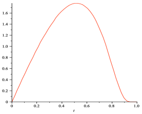
a b

Figure 3. The density (6.2) for (a) $r=2$   and (b) $r=3$.

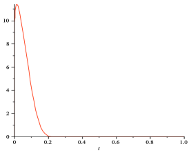
a b

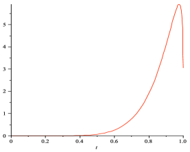
Figure 4. The density (6.2) for (a) $r=1.1$   and (b) $r=8$.

Finally, putting the value of $B$ given in (6.7) into (6.3) we obtain

$${\mathbb{P}}(R\geq x)\leq\exp\left(-\left(\frac{x}{q}\right)^{r^{*}}\frac{1}{A^{r/(r-1)}}\right),$$

which implies that

$$\limsup_{x\to\infty}\frac{\ln{\mathbb{P}}(R\geq x)}{(x/q)^{r^{*}}}\leq-A^{-r/(r-1)}.$$

To get a lower bound for ${\mathbb{P}}(R\geq x)$ we choose $\delta\in(0,\varepsilon)$ as in (2.3). Then, upon passing to the equivalent measure with density proportional to (6.2) we have

$$p_{\delta}\geq dK_{r}\int_{1-\delta}^{1}t^{r-1}\exp\left(-\frac{1}{(1-t^{r})^{1/(r-1)}}\right)dt.$$

Changing variables to $v=(1-t^{r})^{-1/(r-1)}$ yields

$$p_{\delta}\geq K\int_{(1-(1-\delta)^{r})^{-1/(r-1)}}^{\infty}\frac{e^{-v}}{v^{r}}dv,$$

for some constant $K$ whose value is irrelevant. Since for large $v_{0}$, $\int_{v_{0}}^{\infty}\frac{e^{-v}}{v^{r}}dv$ is comparable to $e^{-v_{0}}/v_{0}^{r}$ we get, up to an unimportant constant

$$(1-(1-\delta)^{r})^{r/(r-1)}\exp\left(-\frac{1}{(1-(1-\delta)^{r})^{1/(r-1)}}\right)$$

as the lower bound for $p_{\delta}$. Hence, up to unimportant additive terms

$$\ln p_{\delta}\geq\frac{r}{r-1}\ln\left(1-(1-\delta)^{r}\right)-\frac{1}{(1-(1-\delta)^{r})^{1/(r-1)}}\sim-\frac{1}{(1-(1-\delta)^{r})^{1/(r-1)}},$$

as the second term above is of dominant order for $\delta\to 0$. For small $\delta$ we have

$$1-\left(1-\delta\right)^{r}=1-\exp\left(r\ln(1-\delta)\right)\sim-r\ln(1-\delta),$$

so that upon replacing $\delta$ by $cq/x$ we get that, asymptotically

$$\ln p_{cq/x}\geq-\frac{1}{(-r\ln(1-cq/x))^{1/(r-1)}}\sim-\left(\frac{x}{cqr}\right)^{\frac{1}{r-1}}.$$

Combining this with (2.2) we get that, asymptotically,

$$\ln{\mathbb{P}}(R\geq x) \geq \frac{\ln(1-c)}{\ln(1-cq/x)}\left(-\left(\frac{x}{cqr}\right)^{1/(r-1)}\right)\sim\frac{x\ln(1-c)}{cq}\left(\frac{x}{cqr}\right)^{1/(r-1)}\$$

$$= \left(\frac{x}{q}\right)^{r^{*}}\cdot\frac{\ln(1-c)}{(cr^{1/r})^{r^{*}}}.$$

It follows that

$$\liminf_{x\to\infty}\frac{\ln{\mathbb{P}}(R\geq x)}{(x/q)^{r^{*}}}\geq\frac{C}{r^{1/(r-1)}},\quad\mbox{where}\quad C=\frac{\ln(1-c)}{c^{r^{*}}}<0.$$

$\Box$
Remarks:

(i) The maximal value of $C/r^{1/(r-1)}$ is obtained by setting $c=c_{0}$ where $c_{0}$ is the unique solution of the equation

$$\frac{1}{1-c}+r^{*}\cdot\frac{\ln(1-c)}{c}=0.$$

The uniqueness of the solution is elementary as the function

$$h(c):=\frac{\ln(1-c)}{c^{r^{*}}}$$

approaches $-\infty$ as $c\to 0_{+}$ or $c\to 1_{-}$ and

$$h^{\prime}(c)=-c^{-r^{*}}\left(\frac{1}{1-c}+r^{*}\cdot\frac{\ln(1-c)}{c}\right).$$

The expression in the parentheses, upon letting $y=1/(1-c)$, $y>1$, becomes

$$y-r^{*}\cdot\frac{\ln y}{(y-1)/y}=y\left(1-r^{*}\cdot\frac{\ln y}{y-1}\right).$$

Since $\frac{\ln y}{y-1}$ is decreasing for $y>1$, approaches $1$ as $y\to 1_{+}$ and $0$ as $y\to\infty$ we see that $h^{\prime}(c)$ has exactly one sign change (from positive to negative) on $(0,1)$ and that this change occurs at $c_{0}$ such that

$$\frac{1}{1-c_{0}}+r^{*}\cdot\frac{\ln(1-c_{0})}{c_{0}}=0.$$

While the above equation does not have in general the closed form solution for $c_{0}$ as a function of $r$ (or $r^{*}$), the asymptotic behavior of the constant $C/r^{1/(r-1)}$ as $r$ goes to 0 or $\infty$ can be traced down. Since

$$r^{*}=-\frac{c_{0}}{(1-c_{0})\ln(1-c_{0})},$$

as $r\to\infty$ (and thus $r^{*}\to 1_{+}$) we must have $c_{0}\to 0_{+}$ at the rate $1-c_{0}\sim 1/r^{*}$. But then $c_{0}\sim 1-1/r^{*}=1/r$ and thus

$$\frac{\ln(1-c_{0})}{r^{1/(r-1)}c_{0}^{r^{*}}}\sim\frac{\ln(1-1/r)}{r^{1/(r-1)}(1/r)^{r/(r-1)}}=r\ln(1-1/r)\to-1,\quad\mbox{as\quad$r\to\infty$}.$$

Similarly, if $r\to 1_{+}$ then $c_{0}\to 1_{-}$ in such a way that $1-c_{0}\sim 1/(r^{*}\ln r^{*})$. Then

$$\frac{\ln(1-c_{0})}{r^{1/(r-1)}c_{0}^{r^{*}}}\sim\frac{-\ln(r^{*}\ln r^{*})}{r^{1/(r-1)}(1-1/(r^{*}\ln r^{*}))^{r^{*}}}\sim\frac{-\ln(r^{*}\ln r^{*})}{e}$$

since, as $r\to 1_{+}$

$$r^{1/(r-1)}=\left(1+\frac{1}{1/(r-1)}\right)^{1/(r-1)}\to e,\quad\mbox{and}\quad\left(1-\frac{1}{r^{*}\ln r^{*}}\right)^{r^{*}}\to 1.$$

(ii) It might appear from the argument that the form of density (6.1) was just guessed. While it is true that originally this was the case, there is a heuristic argument which would suggest the same choice. We will explain this heuristics in the next section on a different example, but we would like to mention that following it in the present situation would essentially lead to density given by (6.1).

7. Further example

In this section we present one more example of perpetuity that will have extremely thin tails. Specifically, we will show

Proposition 7.

There exist densities $f_{M}$ for which the perpetuity defined by (3.4) satisfies:

(7.1) $$\forall\ B>q\quad\limsup_{x\to\infty}\frac{\ln{\mathbb{P}}(R\geq x)}{B\exp(x/B)}\leq-\frac{1}{e},$$

and

(7.2) $$\forall\ B<q\quad\liminf_{x\to\infty}\frac{\ln{\mathbb{P}}(R\geq x)}{B\exp(x/B)}\geq\frac{\ln(1-B/q)}{B}.$$

Proof: We consider the case $\Phi(z)=z\ln z$ and we will show that Proposition 3 holds for all $B>q$. It will then follow that for all such $B$

(7.3) $${\mathbb{P}}(R\geq x)\leq\exp(-B\exp(\frac{x}{B}-1)),$$

which will imply (7.1). We will then construct a density of $M$ which, on one hand will guarantee (7.3) and, on the other hand, ensure that $p_{\delta}$ is sufficiently large so that the argument based on Proposition 1 will give (7.2).

To carry out the details of that plan we are to construct a density $f_{M}$ for which

$$e^{qz}\int_{0}^{1}e^{Bzt\ln(zt)}f_{M}(t)dt\leq e^{Bz\ln z}.$$

This is equivalent to

$$e^{qz}\int_{0}^{1}e^{-B(1-t)z\ln z}t^{Btz}f_{M}(t)dt\leq 1,$$

and it is enough to construct an $f_{M}$ for which

$$e^{qz}\int_{0}^{1}e^{-B(1-t)z\ln z}f_{M}(t)dt=e^{qz}\int_{0}^{1}e^{-Btz\ln z}f_{M}(1-t)dt\leq 1.$$

We now set $f_{M}(1-t)=K\exp(-h(t)),$ where $h$ is a non–negative function and $K^{-1}=\int_{0}^{1}\exp(-h(t))dt$. The inequality to be established becomes

(7.4) $$e^{qz}\int_{0}^{1}e^{-Btz\ln z-h(t)}dt\leq\int_{0}^{1}e^{-h(t)}dt.$$

One is guided to a reasonable choice of $h$ by the following heuristics. Suppose $h$ is differentiable and chosen so that

(7.5) $$Btz\ln z+h(t)$$

is minimized at its critical point $t=t_{z}\in(0,1)$ which thus satisfies

(7.6) $$Bz\ln z+h^{\prime}(t_{z})=0.$$

Then the left–hand side of (7.4) is no more than

$$\exp\left(qz-Bt_{z}z\ln z-h(t_{z})\right)\leq\exp\left(z(q-Bt_{z}\ln z)\right).$$

Since we must be able to make it arbitrarily negative (by increasing $B$ if necessary) we should require that $t_{z}\ln z$ is about a constant, say $t_{z}=1/\ln z$ for $z>e$. Substituting this into (7.6) yields

$$h^{\prime}\left(1/\ln z\right)=-z\ln z,\quad\mbox{or\quad with $s=1/\ln z$,}\quad h^{\prime}(s)=-\frac{e^{1/s}}{s}.$$

Thus we may take

$$h(t)=\int_{t}^{1}\frac{e^{1/s}}{s}ds,$$

and we obtain

$$f_{M}(t)=K\exp\left(-\int_{1-t}^{1}\frac{e^{1/s}}{s}ds\right),\quad 0<t<1,\quad\mbox{where}\quad K^{-1}=\int_{0}^{1}e^{-h(u)}du.$$

(Note that $t_{z}$ is indeed the local minimum of (7.5).) A graph of the density $f_{M}$ is given in Figure 5.

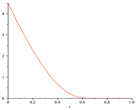
a b

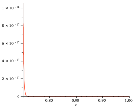
Figure 5. (a) The density $f_{M}$  and (b) its detail closer to 1.

For the lower bound, as

$$p_{\delta}=K\int_{1-\delta}^{1}e^{-h(1-t)}dt=K\int^{\delta}_{0}e^{-h(t)}dt,$$

we obtain

$$\ln{\mathbb{P}}(R\geq x) = \frac{\ln(1-c)}{\ln(1-cq/x)}\ln\left(K\int_{0}^{cq/x}e^{-h(t)}dt\right)$$

$$\sim -\frac{\ln(1-c)}{cq}x\ln\left(\int_{0}^{cq/x}e^{-h(t)}dt\right).$$

We need the following lemma which we justify below.

Lemma 8.

(7.7) $$\frac{y\ln\left(\int_{0}^{1/y}e^{-h(t)}dt\right)}{e^{y}}\to-1,\quad\mbox{as}\quad y\to\infty.$$

Using this lemma with $y=x/(cq)$ and $c=B/q$ we get, asymptotically,

$$\frac{\ln{\mathbb{P}}(R\geq x)}{e^{x/B}}\geq-\frac{\ln(1-B/q)}{Be^{x/B}}x\ln\left(\int_{0}^{B/x}e^{-h(t)}dt\right)\sim\ln(1-B/q),$$

which implies (7.2). $\Box$

Proof of Lemma 8: We re-write the left–hand side of (7.7) as

$$\frac{\ln\left(\int_{0}^{1/y}e^{-h(t)}dt\right)}{e^{y}/y},$$

and apply l’Hospital rule. The first differentiation gives

$$\frac{(-1/y^{2})e^{-h(1/y)}}{\left(\int_{0}^{1/y}e^{-h(t)}dt\right)\left(-e^{y}/y^{2}+e^{y}/y\right)}=\frac{e^{-h(1/y)}e^{-y}/(1-y)}{\int_{0}^{1/y}e^{-h(t)}dt}.$$

Differentiating again we get

$$\frac{(1/y^{2})h^{\prime}(1/y)e^{-h(1/y)}e^{-y}/(1-y)+e^{-h(1/y)}\frac{d}{dy}\left(e^{-y}/(1-y)\right)}{(-1/y^{2})e^{-h(1/y)}}$$

$$\quad=-h^{\prime}\left(\frac{1}{y}\right)\frac{e^{-y}}{1-y}-y^{2}\frac{d}{dy}\left(\frac{e^{-y}}{1-y}\right).$$

Since $h^{\prime}(s)=-e^{1/s}/s$ the first term goes to $-1$ as $y\to\infty$ while the second is $o(1)$. $\Box$

References

[1]
G. Alsmeyer, A. Iksanov, and U. Rösler.
On distributional properties of perpetuities.
J. Theoret. Probab., 20:666–682, 2009.
[2]
M. Białkowski and J. Wesołowski.
Asymptotic behavior of some random splitting schemes.
Probab. Math. Statist., 22:181–191, 2002.
[3]
L. Bondesson.
A general result on infinite divisibility.
Ann. Probab., 7(6):965–979, 1979.
[4]
M. Brown.
Error bounds for exponential approximations of geometric
convolutions.
Ann. Probab., 18(3):1388–1402, 1990.
[5]
J.-F. Chamayou and G. Letac.
Explicit stationary distributions for compositions of random
functions and products of random matrices.
J. Theoret. Probab., 4:3–36, 1991.
[6]
P. Embrechts and C. M. Goldie.
Perpetuities and random equations.
In Asymptotic statistics (Prague, 1993), Contrib. Statist.,
pages 75–86. Physica, Heidelberg, 1994.
[7]
C. M. Goldie.
Implicit renewal theory and tails of solutions of random equations.
Ann. Appl. Probab., 1(1):126–166, 1991.
[8]
C. M. Goldie and R. Grübel.