Vortex pairing in two-dimensional Bose gases

Abstract

Recent experiments on ultracold Bose gases in two dimensions have provided evidence for the existence of the Berezinskii-Kosterlitz-Thouless (BKT) phase via analysis of the interference between two independent systems. In this work we study the two-dimensional quantum degenerate Bose gas at finite temperature using the projected Gross-Pitaevskii equation classical field method. While this describes the highly occupied modes of the gas below a momentum cutoff, we have developed a method to incorporate the higher momentum states in our model. We concentrate on finite-sized homogeneous systems in order to simplify the analysis of the vortex pairing. We determine the dependence of the condensate fraction on temperature and compare this to the calculated superfluid fraction. By measuring the first order correlation function we determine the boundary of the Bose-Einstein condensate and BKT phases, and find it is consistent with the superfluid fraction decreasing to zero. We reveal the characteristic unbinding of vortex pairs above the BKT transition via a coarse-graining procedure. Finally, we model the procedure used in experiments to infer system correlations [Hadzibabic et al., Nature 441, 1118 (2006)], and quantify its level of agreement with directly calculated in situ correlation functions.

I Introduction

At low temperatures a three-dimensional (3D) Bose gas can undergo a phase transition to a Bose-Einstein condensate. In contrast, thermal fluctuations prevent a two-dimensional (2D) Bose gas from making a phase transition to an ordered state, in accordance with the Mermin-Wagner-Hohenberg theorem Mermin and Wagner (1966); Hohenberg (1967). However, the 2D Bose gas supports topological defects in the form of vortices, and in the presence of interactions can instead undergo a Berezinskii-Kosterlitz-Thouless (BKT) Berezinskii (1971); Kosterlitz and Thouless (1973); Posazhennikova (2006) transition to a quasi-coherent superfluid state. The BKT transition was first observed in liquid helium thin films Bishop and Reppy (1978), however, more recently, evidence for this transition has been found in dilute Bose gases Stock et al. (2005); Hadzibabic et al. (2006); Krüger et al. (2007); Schweikhard et al. (2007); Cladé et al. (2009) (also see Görlitz et al. (2001); Smith et al. (2005)).

Ultracold gases have proven to be beautiful systems for making direct comparisons between experiment and ab initio theory. Experiments in the 2D regime present a new challenge for theory as strong fluctuations invalidate mean-field theories (e.g. see Prokof’ev et al. (2001); Prokof’ev and Svistunov (2002); Posazhennikova (2006); Bisset and Blakie (2009); Mathey and Polkovnikov (2009); Sato et al. (2009); Gies and Hutchinson (2004); Schumayer and Hutchinson (2007)), and only recently have quantum Monte Carlo Holzmann and Krauth (2008); Holzmann et al. (2009) and classical field (c-field) Simula and Blakie (2006); Simula et al. (2008); Bisset et al. (2009) methods been developed that are directly applicable to the experimental regime.

In this paper we study a uniform Bose gas of finite spatial extent and parameters corresponding to current experiments. To analyze this system we use the projected Gross-Pitaevskii equation (PGPE), a c-field technique suited to studying finite temperature Bose fields with many highly occupied modes. We develop a technique for extracting the superfluid density based on linear response properties, and use this to understand the relationship between superfluidity and condensation in the finite system.

With this formalism we then examine two important applications: First, we provide a quantitative validation of the interference technique used in the ENS experiment to determine the nature of two-point correlation in the system. To do this we simulate the interference pattern generated by allowing two independent 2D systems to expand and interfere. Then applying the experimental fitting procedure to analyze the interference pattern we can extract the inferred two point correlations, which we can then compare against the in situ correlations that we calculate directly. Second, we examine the correlations between vortices and antivortices in the system to directly quantify the emergence of vortex-antivortex pairing in the low temperature phase. A similar study was made by Giorgetti et al. using a semiclassical field technique Giorgetti et al. (2007). We find results for vortex number and vortex pair distributions consistent with their results, and we show how a coarse graining procedure can be used to reveal the unpaired vortices in the system.

We now briefly outline the structure of this paper: In Sec. II we review the 2D Bose gas and relevant BKT physics. In Sec. III we outline the c-field technique and how it is specialized to describing a uniform, but finite, 2D Bose gas. In Sec. IV we present our main results, before concluding.

II Formalism

Here we consider a dilute 2D Bose gas described by the Hamiltonian

$$\hat{H}=\int d^{2}\mathbf{x}\,\hat{\psi}^{\dagger}\left\{-\frac{\hbar^{2}\nabla^{2}_{\mathbf{x}}}{2m}\right\}\hat{\psi}+\frac{\hbar^{2}g}{2m}\int d^{2}\mathbf{x}\,\hat{\psi}^{\dagger}\hat{\psi}^{\dagger}\hat{\psi}\hat{\psi},$$ (1)

where $m$ is the atomic mass, $\mathbf{x}=(x,y)$, and $\hat{\psi}=\hat{\psi}(\mathbf{x})$ is the bosonic field operator.

We take the two-dimensional geometry to be realized by tight confinement in the $z$ direction that restricts atomic occupation to the lowest $z$ mode. The dimensionless 2D coupling constant is

$${g}=\frac{\sqrt{8\pi}a}{a_{z}},$$ (2)

with $a_{z}$ the spatial extent of the $z$ mode and $a$ the s-wave scattering length. We will assume that $a_{z}\gg a$ so that the scattering is approximately three-dimensional Petrov et al. (2000), a condition well-satisfied in the ENS and NIST experiments Stock et al. (2005); Hadzibabic et al. (2006); Krüger et al. (2007); Cladé et al. (2009). For reference, the ENS experiment reported in Hadzibabic et al. (2006) had ${g}\approx 0.15$, whereas in the NIST experiments ${g}\approx 0.02$ Cladé et al. (2009).

In contrast to experiments we focus here on the uniform case; no trapping potential in the $xy$ plane is considered. We perform finite sized calculations corresponding to a square system of size $L$ with periodic boundary conditions. Working in the finite size regime simplifies the simulations and is more representative of current experiments. We note that the thermodynamic limit corresponds to taking $L\to\infty$ while keeping the density, $n=\langle\hat{\psi}^{\dagger}\hat{\psi}\rangle$, constant.

II.1 Review of BKT physics

The BKT superfluid phase has several distinctive characteristics, which we briefly review.

II.1.1 First order correlations

Below the BKT transition the first-order correlations decay according to an inverse power law:

$$g^{(1)}(\mathbf{x},\mathbf{x}^{\prime})\propto\lVert\mathbf{x}-\mathbf{x}^{\prime}\rVert^{-\alpha}.$$ (3)

Systems displaying such algebraic decay are said to exhibit quasi-long-range order Chaikin and Lubensky (1995). This is in contrast to both the high temperature (disordered phase) in which the correlations decay exponentially, and long-range ordered case of the 3D Bose gas in which $g^{(1)}\to\rm{const.}$ for $\lVert\mathbf{x}-\mathbf{x}^{\prime}\rVert\to\infty$.

II.1.2 Superfluid density

Nelson and Kosterlitz Nelson and Kosterlitz (1977) found that the exponent of the algebraic decay is related to the ratio of the superfluid density and temperature. To within logarithmic corrections

$$\alpha(T)=\frac{1}{\lambda^{2}\rho_{s}(T)},$$ (4)

where $\rho_{s}$ is the superfluid density and $\lambda=h/\sqrt{2\pi mk_{B}T}$ is the thermal de Broglie wavelength. Furthermore, Nelson and Kosterlitz showed that this ratio converges to a universal constant as the transition temperature, $T_{\text{KT}}$, is approached from below: $\lim_{T\to T_{\text{KT}}^{-}}\alpha(T)=1/4$ (i.e., $\rho_{s}\lambda^{2}=4$). Thus, the superfluid fraction undergoes a universal jump from $\rho_{s}(T_{\text{KT}}^{+})=0$ to $\rho_{s}(T_{\text{KT}}^{-})=4/\lambda^{2}$ as the temperature decreases through $T_{\text{KT}}$.

II.1.3 Vortex binding transition

Another important indicator of the BKT transition is the behavior of topological excitations, which are quantized vortices and antivortices in the case of a Bose gas. A single vortex has energy which scales with the logarithm of the system size. At low temperatures this means that the free energy for a single vortex is infinite (in the thermodynamic limit), and vortices cannot exist in isolation. As originally argued in Kosterlitz and Thouless (1973), the entropic contribution to the free energy also scales logarithmically with the system size, and will dominate the free energy at high temperatures allowing unbound vortices to proliferate. This argument provides a simple estimate for the BKT transition temperature.

Although unbound vortices are thermodynamically unfavored at $T<T_{\text{KT}}$, bound pairs of counter-rotating vortices may exist since the total energy of such a pair is finite . This leads to a distinctive qualitative characterization of the BKT transition: as the temperature increases through $T_{\text{KT}}$ pairs of vortices unbind.

II.1.4 Location of the BKT transition in the dilute Bose gas

While the relation $\rho_{s}(T_{\text{KT}}^{-})=4/\lambda^{2}$ between the superfluid density and temperature at the transition is universal, the total density, $n$, at the transition is not. General arguments Popov (1983); Kagan et al. (1987); Fisher and Hohenberg (1988) suggest that the transition point for the dilute uniform 2D Bose gas is given by

$$(n\lambda^{2})_{\text{KT}}=\ln\left(\frac{\xi}{{g}}\right),$$ (5)

where $\xi$ is a constant. Prokofév, Ruebenacker and Svistunov Prokof’ev et al. (2001); Prokof’ev and Svistunov (2002) studied the homogeneous Bose gas using Monte Carlo simulations of an equivalent classical $\phi^{4}$ model on a lattice. Using an extrapolation to the infinite-sized system, they computed a value for the dimensionless constant, $\xi=380\pm 3$. By inverting Eq. (5), we obtain the BKT critical temperature for the infinite system

$$T_{\text{KT}}^{\infty}=\frac{2\pi\hbar^{2}n}{mk_{B}\ln\left(\xi\hbar^{2}/m{g}\right)}.$$ (6)

We use the superscript $\infty$ to indicate that this result holds in the thermodynamic limit.

III Method

III.1 c-field and incoherent regions

We briefly outline the PGPE formalism, which is developed in detail in Ref. Blakie et al. (2008). The Bose field operator is split into two parts according to

$$\hat{\psi}(\mathbf{x})=\psi_{\text{\bf{C}}}(\mathbf{x})+\hat{\psi}_{\text{\bf{I}}}(\mathbf{x}),$$ (7)

where $\psi_{\text{\bf{C}}}$ is the coherent region c-field  and $\hat{\psi}_{\text{\bf{I}}}$ is the incoherent field operator (see Blakie et al. (2008)). These fields are defined as the low and high energy projections of the full quantum field operator, separated by the cutoff wave vector $K$. In our theory this cutoff is implemented in terms of the plane wave eigenstates $\{\varphi_{\mathbf{n}}(\mathbf{x})\}$ of the time-independent single particle Hamiltonian, that is,

$$\varphi_{\mathbf{n}}(\mathbf{x}) =\frac{1}{{L}}e^{-i\mathbf{k}_{\mathbf{n}}\cdot\mathbf{x}},$$ (8)

$$\mathbf{k}_{\mathbf{n}} =\frac{\pi}{L}\mathbf{n},$$ (9)

with $\mathbf{n}=(n_{x},n_{y})\in\mathbb{Z}^{2}$. The fields are thus defined by

$$\psi_{\text{\bf{C}}}(\mathbf{x}) \equiv\sum_{\mathbf{n}\in\text{\bf{C}}}c_{\mathbf{n}}\varphi_{\mathbf{n}}(\mathbf{x}),$$ (10)

$$\hat{\psi}_{\text{\bf{I}}}(\mathbf{x}) \equiv\sum_{\mathbf{n}\in\text{\bf{I}}}\hat{a}_{\mathbf{n}}\varphi_{\mathbf{n}}(\mathbf{x}),$$ (11)

where the $\hat{a}_{\mathbf{n}}$ are Bose annihilation operators, the $c_{\mathbf{n}}$ are complex amplitudes, and the sets of quantum numbers defining the regions are

C $$=\{\mathbf{n}:\lVert\mathbf{k}_{\mathbf{n}}\rVert\leq K\},$$ (12)

I $$=\{\mathbf{n}:\lVert\mathbf{k}_{\mathbf{n}}\rVert>K\}.$$ (13)

III.1.1 Choice of C region

In general, the applicability of the PGPE approach to describing the finite temperature gas relies on an appropriate choice for $K$, so that the modes at the cutoff have an average occupation of order unity. In this work we choose an average of five or more atoms per mode using a procedure discussed in appendix A. This choice means that all the modes in C are appreciably occupied, justifying the classical field replacement $\hat{a}_{\mathbf{n}}\to c_{\mathbf{n}}$. In contrast the I region contains many sparsely occupied modes that are particle-like and would be poorly described using a classical field approximation. Because our 2D system is critical over a wide temperature range, additional care is needed in choosing C. Typically strong fluctuations occur in the infrared modes up to the energy scale $\hbar^{2}gn/m$. Above this energy scale the modes are well described by mean-field theory (e.g. see the discussion in Kashurnikov et al. (2001); Prokof’ev et al. (2001)). For the results we present here, we have

$$\frac{\hbar^{2}K^{2}}{2m}\gtrsim\frac{\hbar^{2}g}{m}n$$ (14)

for simulations around the transition region and at high temperature. At temperatures well below $T_{\text{KT}}$, the requirement of large modal occupation near the cutoff competes with this condition and we favor the former at the expense of violating Eq. (14).

III.1.2 PGPE treatment of C region

The equation of motion for $\psi_{\text{\bf{C}}}$ is the PGPE

$$i\hbar\frac{\partial\psi_{\text{\bf{C}}}}{\partial t}=-\frac{\hbar^{2}\nabla^{2}_{\mathbf{x}}}{2m}\psi_{\text{\bf{C}}}+\frac{\hbar^{2}g}{m}\mathcal{P}_{\text{\bf{C}}}\left\{\lvert\psi_{\text{\bf{C}}}\rvert^{2}\psi_{\text{\bf{C}}}\right\},$$ (15)

where the projection operator

$$\mathcal{P}_{\text{\bf{C}}}\{F(\mathbf{x})\}\equiv\sum_{\mathbf{n}\in\text{\bf{C}}}\varphi_{\mathbf{n}}(\mathbf{x})\int d^{2}\mathbf{x}^{\prime}\,\varphi_{\mathbf{n}}^{*}(\mathbf{x}^{\prime})F(\mathbf{x}^{\prime}),\\$$ (16)

formalizes our basis set restriction of $\psi_{\text{\bf{C}}}$ to the C region. The main approximation used to arrive at the PGPE is to neglect dynamical couplings to the incoherent region Davis et al. (2001a).

We assume that Eq. (15) is ergodic Davis et al. (2001b), so that the microstates {$\psi_{\text{\bf{C}}}$} generated through time evolution form an unbiased sample of the equilibrium microstates. Time averaging can then be used to obtain macroscopic equilibrium properties. We generate the time evolution by solving the PGPE with three adjustable parameters: (i) the cutoff wave vector, $K$, that defines the division between C and I, and hence the number of modes in the C region; (ii) the number of C region atoms, $N_{\text{\bf{C}}}$; (iii) the total energy of the C region, $E_{\text{\bf{C}}}$. The last two quantities, defined as

$$E_{\text{\bf{C}}} =\int d^{2}\mathbf{x}\,\psi_{\text{\bf{C}}}^{*}\left(-\frac{\hbar^{2}\nabla^{2}_{\mathbf{x}}}{2m}+\frac{\hbar^{2}g}{2m}\lvert\psi_{\text{\bf{C}}}\rvert^{2}\right)\psi_{\text{\bf{C}}},$$ (17)

$$N_{\text{\bf{C}}} =\int d^{2}\mathbf{x}\,\lvert\psi_{\text{\bf{C}}}(\mathbf{x})\rvert^{2},$$ (18)

are important because they represent constants of motion of the PGPE (15), and thus control the thermodynamic equilibrium state of the system.

III.1.3 Obtaining equilibrium properties for the C region

To characterize the equilibrium state in the C region it is necessary to determine the average density, temperature and chemical potential, which in turn allow us to characterize the I region (see Sec. III.2). These and other C region quantities can be computed by time-averaging, e.g, the average C region density is given by

$$n_{\text{\bf{C}}}(\mathbf{x})\approx\frac{1}{M_{s}}\sum_{j=1}^{M_{s}}\left\lvert\psi_{\text{\bf{C}}}(\mathbf{x},t_{j})\right\rvert^{2},$$ (19)

where $\{t_{j}\}$ is a set of $M_{s}$ times (after the system has been allowed to relax to equilibrium) at which the field is sampled. We typically use 2000 samples from our simulation to perform such averages over a time of $\sim 16$ s. Another quantity of interest here is the first order correlation function, which we calculate directly via the expression

$$G^{(1)}_{\text{\bf{C}}}(\mathbf{x},\mathbf{x}^{\prime})\approx\frac{1}{M_{s}}\sum_{j=1}^{M_{s}}\psi_{\text{\bf{C}}}^{*}(\mathbf{x},t_{j})\psi_{\text{\bf{C}}}(\mathbf{x}^{\prime},t_{j}).$$ (20)

Derivatives of entropy, such as the temperature ($T$) and chemical potential ($\mu_{\text{\bf{C}}}$) can be calculated by time averaging appropriate quantities constructed from the Hamiltonian (17) using the Rugh approach Rugh (1997). The detailed implementation of the Rugh formalism for the PGPE is rather technical and we refer the reader to Refs. Davis and Morgan (2003); Davis and Blakie (2005) for additional details of this procedure.

A major extension to the formalism of the PGPE made in this work is the development of a method for extracting the superfluid fraction, $\rho_{s}$, from these calculations. For this we use linear response theory to relate the superfluid fraction to the long wavelength limit of the second order momentum density correlations. An extensive discussion of this approach, and the numerical methods used to implement it, are presented in appendix D.

III.2 Mean-field treatment of I region

Occupation of the I region modes, $N_{\text{\bf{I}}}$, accounts for about 25% of the total number of atoms at temperatures near the phase transition. We assume a time independent state for the I region atoms defined by a Wigner function Naraschewski and Glauber (1999), allowing us to calculate quantities of interest by integrating over the above-cutoff momenta, $k>K$ Bezett et al. (2008); Davis and Blakie (2006).

Our assumed Wigner function corresponds to the self-consistent Hartree-Fock theory as applied in Davis and Blakie (2006). In two dimensions this is

$$W_{\text{\bf{I}}}(\mathbf{k},\mathbf{x})=\frac{1}{(2\pi)^{2}}\frac{1}{e^{(E_{\text{HF}}(\mathbf{k})-\mu)/k_{B}T}-1},$$ (21)

where

$$E_{\text{HF}}(\mathbf{k})=\frac{\hbar^{2}\mathbf{k}^{2}}{2m}+\frac{2\hbar^{2}g}{m}(n_{\text{\bf{C}}}+n_{\text{\bf{I}}}),$$ (22)

is the Hartree-Fock energy, $n_{\text{\bf{I}}}$ is the I region density, and $\mu=\mu_{\text{\bf{C}}}+2\hbar^{2}gn_{\text{\bf{I}}}/m$ is the chemical potential (shifted by the mean-field interaction with the I region atoms). Note that the average densities are constant in the uniform system, so $W_{\text{\bf{I}}}(\mathbf{k},\mathbf{x})$ has no explicit $\mathbf{x}$ dependence, however, we include this variable for generality when defining the associated correlation function.

The I region density appearing in Eq. (22) is given by

$$n_{\text{\bf{I}}}=\int_{\lVert\mathbf{k}\rVert\geq K}d^{2}\mathbf{k}\,W_{\text{\bf{I}}}(\mathbf{k},\mathbf{x}),$$ (23)

with corresponding atom number $N_{\text{\bf{I}}}=n_{\text{\bf{I}}}L^{2}$; total number is simply

$$N=N_{\text{\bf{C}}}+N_{\text{\bf{I}}}.$$ (24)

An analytic expression for $n_{\text{\bf{I}}}$ and simplified procedure for numerically calculating the first order correlation function of the I region atoms, $G^{(1)}_{\text{\bf{I}}}$, can be obtained by taking integrals over the phase space. These results are discussed in appendix B.

III.3 Equilibrium configurations with fixed $T$ and $N$

Generating equilibrium classical fields with given values of $E_{\text{\bf{C}}}$ and $N_{\text{\bf{C}}}$ is straightforward since the PGPE simulates a microcanonical system (see appendix A.3). However, we wish to simulate systems with a given temperature and total number. As described in the preceding two sections these can only be determined after a simulation has been performed. In appendix A we outline a procedure for estimating values of $E_{\text{\bf{C}}}$ and $N_{\text{\bf{C}}}$ for desired values of $N$ and $T$ based on a root finding scheme using a Hartree-Fock-Bogoliubov analysis for the initial guess.

IV Results

We choose simulation parameters in analogy with the Paris experiment of Hadzibabic et al. Hadzibabic et al. (2006). This experiment used an elongated atomic cloud of approximately $10^{5}$ ⁸⁷Rb atoms, with a spatial extent (Thomas-Fermi lengths) of 120 $\mu$m and 10 $\mu$m along the two loosely trapped $x$ and $y$ directions. The tight confinement in the $z$ direction was provided by an optical lattice.

Although our simulation is for a uniform system, we have chosen similar parameters where possible. Our primary simulations are for a system in a square box with $L=100$ $\mu$m, with $4{\times}10^{5}$ ⁸⁷Rb atoms. We also present results for systems with $L=50$ $\mu$m and $L=200$ $\mu$m at the same density in order to better understand finite-size effects. All simulations are for the case of $g=0.15$ corresponding to the experimental parameters reported in Hadzibabic et al. (2006).

The cutoff wave vector $K$ varied with temperature to ensure appropriate occupation of the highest modes (see Sec. III.1.1). For the 100 $\mu$m system, the number of C region modes ranged between 559 at low temperatures to 11338 at the highest temperature studied.

IV.1 Simulation of expanded interference patterns between two systems

In order to make a direct comparison with the experimental results of Hadzibabic et al. (2006), we have generated synthetic interference patterns and implemented the experimental analysis technique. Our simulated imaging geometry is identical to that found in Hadzibabic et al. (2006), with expansion occurring in the $z$-direction. The interference pattern is formed in the $x$-$z$ plane via integration of the density along the $y$-direction (“absorption imaging”).

Our algorithm for obtaining the interference pattern due to our classical field is very similar to that presented in Hadzibabic et al. (2004). Our above cutoff thermal cloud is taken into account separately. We consider a pair of fields $\psi_{\text{\bf{C}}}^{(1)}(x,y),\psi_{\text{\bf{C}}}^{(2)}(x,y)$ from different times during the simulation, chosen such that the fields can be considered independent. The 3D wavefunction corresponding to each field is reconstructed by assuming a harmonic oscillator ground state in the tight-trapping direction. These two reconstructed fields are spatially separated by $\Delta=3$ $\mu$m, corresponding to the period of the optical lattice in Hadzibabic et al. (2004).

Given this initial state, we neglect atomic interactions and only account for expansion in the tightly-trapped direction. This yields a simple analytical result for the full classical field $\psi_{\text{\bf{C}}}(x,y,z,\tau)$ at later times. The contribution of the above-cutoff atoms is included by an incoherent addition of intensities. The result is integrated along the $y$-direction to simulate the effect of absorption imaging with a laser beam, that is,

$$n_{\rm{im}}(x,z) =\int_{0}^{L^{\prime}}dy\,\Big{[}\big{\lvert}\psi_{\text{\bf{C}}}^{(T)}(x,y,z,\tau)\big{\rvert}^{2}+n_{\text{\bf{I}}}(x,y,z,\tau)\Big{]},$$ (25)

$$\psi_{\text{\bf{C}}}^{(T)} =\psi_{\text{\bf{C}}}^{(1)}(x,y,z,\tau)+\psi_{\text{\bf{C}}}^{(2)}(x\!-\!\Delta,y,z,\tau).$$ (26)

Rather than integrate the full field along the $y$-direction, we use only a slice of length $L^{\prime}=10$ $\mu$m in keeping with the experimental geometry of Ref. Hadzibabic et al. (2006).

The interference patterns, $n_{\rm{im}}(x,z)$, generated this way contained fine spatial detail not seen in the experimental images. To make a more useful comparison to experiment it is necessary to account for the finite optical imaging resolution by applying a Gaussian convolution in the $x$-$z$ plane with standard deviation 3 $\mu$m. Had .

In accordance with the Paris experiment, we use a 22 ms expansion time to generate interference patterns for quantitative analysis (see Sec. IV.3.2). To obtain characteristic interference images for display in Hadzibabic et al. (2006), the experiments used a shorter 11 ms expansion Had . We exhibit examples of interference patterns at various temperatures in Fig. 1, for this shorter expansion time. These images show a striking resemblance to the results presented in Ref. Hadzibabic et al. (2006).

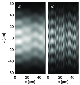
Figure 1: Synthetic interference patterns generated from the 50 $\mu$m grid by simulation of the experimental procedure of Ref. Hadzibabic et al. (2006). (a) At low temperatures, $T\approx 0.5T_{\text{KT}}$, the interference fringes are straight. (b) Just below the transition temperature, $T\approx 0.95T_{\text{KT}}$, the fringes become wavy due to decreased spatial phase coherence. Phase dislocations become common at temperatures above the transition, (c) $T\approx 1.05T_{\text{KT}}$, and (d) $T\approx 1.1T_{\text{KT}}$. These “zipper patterns” indicate the presence of free vortices. (e) When simulation of the finite imaging resolution is disabled, the zipper patterns from the field in sub figure (d) are no longer clearly visible; the high-frequency details obscure the phase information without providing obvious additional information about the existence of vortex pairs.

IV.2 Condensate and superfluid fractions

For a 2D Bose gas in a box we expect a nonzero condensate fraction due to the finite spacing of low-energy modes. A central question is whether we can observe a distinction between the crossover due to Bose condensation and that due to BKT physics. To address this question we have computed both the condensate and superfluid fractions from our dynamical simulations.

The condensate fraction in a homogeneous system is easily identified as the average fractional occupation of the lowest momentum mode. This is directly available from our simulations as a time average of the $\mathbf{k}=\mathbf{0}$ mode of the classical field,

$$f_{c}=\left\langle c_{\mathbf{0}}^{*}c_{\mathbf{0}}^{\vphantom{*}}\right\rangle/N.$$ (27)

Extracting the superfluid fraction from dynamical classical field simulations provides a more difficult challenge. For this we use linear response theory to relate the superfluid fraction to the long wavelength limit of the second order momentum density correlations. Details concerning the technique are given in appendix D.

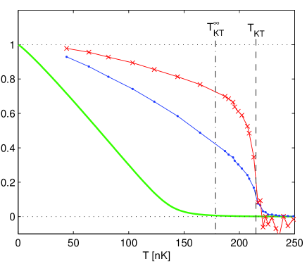
Figure 2: (color online). Condensate fraction (solid dots) and superfluid fraction (crosses) as functions of temperature for the 100 $\mu$m² grid. The transition temperature in the thermodynamic limit, $T_{\text{KT}}^{\infty}$ Prokof’ev et al. (2001), is shown as a vertical dot-dashed line. The vertical dashed line shows our estimate for the transition temperature in the finite system. The thick solid line is the condensate fraction for an ideal Bose gas in the grand canonical ensemble with the same number of atoms and periodic spatial domain. The superfluid fraction becomes negative in places because the extrapolation of the momentum correlations to $\mathbf{k}=0$ is sensitive to statistical noise at high temperature (see appendix D.2 for details).

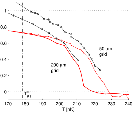
Figure 3: (color online). Detail of the superfluid fraction near the transition temperature. Solid dots represent the calculation based on momentum correlations as described in appendix D. Results for the largest and smallest grids are shown (left and right, respectively). The data for the 100 $\mu$m grid is omitted for clarity, but lies between the curves shown as expected. Open circles represent the calculation of the superfluid fraction from the associated fitted values for the decay coefficient $\alpha$, via Eq. (4). The open circles terminate where the power law fitting procedure fails.

Figure 2 compares the results for the superfluid and condensate fractions computed on the 100 $\mu$m grid. These results are qualitatively similar to the results for the larger and smaller grids. In particular, we note that there is no apparent separation between temperatures at which the superfluid and condensate fractions fall to zero. Also shown in Fig. 2 is the condensate fraction for the ideal Bose gas confined to an identical finite-size box in the grand canonical ensemble. The large shift between ideal and computed transition temperatures indicates the effect of interactions in the 2D system. Because the average system density is uniform, this large shift is to due to critical fluctuations (also see Kashurnikov et al. (2001)).

In our calculations we identify the transition temperature, $T_{\text{KT}}$, as where the superfluid fraction falls off most rapidly (i.e., the location of steepest slope on the $\rho_{s}$ versus $T$ graph; see Fig. 2). As the system size increases, this transition temperature moves toward the value for an infinite-sized system, $T_{\text{KT}}^{\infty}$ Prokof’ev et al. (2001). This effect is illustrated by the behavior of the superfluid fraction in Fig. 3.

IV.3 First order correlations — algebraic decay

Algebraic decay of the first order correlations, as described by Eq. (3), is a characteristic feature of the BKT phase. Above the BKT transition, the first order correlations should revert to the exponential decay expected in a disordered phase.

The normalized first order correlation function, $g^{(1)}$ is defined by

$$g^{(1)}(\mathbf{x},\mathbf{x}^{\prime})=\frac{G^{(1)}(\mathbf{x},\mathbf{x}^{\prime})}{\sqrt{n(\mathbf{x})n(\mathbf{x}^{\prime})}},$$ (28)

where $G^{(1)}(\mathbf{x},\mathbf{x}^{\prime})=\big{\langle}\hat{\psi}^{\dagger}(\mathbf{x})\hat{\psi}(\mathbf{x^{\prime}})\big{\rangle}$ is the unnormalized first order correlation function Naraschewski and Glauber (1999).

IV.3.1 Direct calculation of $g^{(1)}$

In the PGPE formalism the C and I contributions to the correlation function are additive Bezett et al. (2008), that is,

$$G^{(1)}(\mathbf{x},\mathbf{x}^{\prime})=G^{(1)}_{\text{\bf{C}}}(\mathbf{x},\mathbf{x}^{\prime})+G^{(1)}_{\text{\bf{I}}}(\mathbf{x},\mathbf{x}^{\prime}),$$ (29)

where $G^{(1)}_{\text{\bf{C}}}$ and $G^{(1)}_{\text{\bf{I}}}$ are defined in Eqs. (20) and (49), respectively. It is interesting to note that $G^{(1)}_{\text{\bf{C}}}$ and $G^{(1)}_{\text{\bf{I}}}$ individually display an oscillatory decay behavior — originating from the cutoff — an effect which correctly cancels when the two are added together.

Having calculated $g^{(1)}$, we obtain the coefficient $\alpha$ by fitting the algebraic decay law, Eq. (3), using nonlinear least squares; sample fits are shown in Fig. 4. The fit is conducted over the region between 10 and 40 de Broglie wavelengths. The short length scale cutoff is to avoid the contribution of the non-universal normal atoms, for which the thermal de Broglie wavelength sets the appropriate decay length. The long distance cutoff is chosen to be small compared to the length scale $L$, to avoid the effect of periodic boundary conditions on the long range correlations.

The quality of the fitting procedure, and the breakdown of expression (3) at the BKT transition can be observed by adding an additional degree of freedom to the fitting function. In particular, at each temperature we fit the quadratic $\ln(g^{(1)})=A-\tilde{\alpha}\ln(x)+\delta\ln^{2}(x)$ and extract the parameter $\delta$ ($\tilde{\alpha}\approx\alpha$ is discarded). The abrupt failure of the fits can be observed in the inset of Fig. 5 as a sudden increase in the value of $\lvert\delta(T)\rvert$ — an effect which is in excellent agreement with the value of $T_{\text{KT}}$ as estimated from the superfluid fraction.

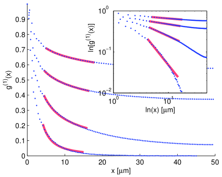
Figure 4: (color online). Sample fits to the algebraic decay of $g^{(1)}$ at various temperatures, ranging from below to above the transition. High temperatures correspond to curves at the bottom of the figure which have rapid falloff of $g^{(1)}$ with distance. Fits are shown on a log-log scale in the inset to emphasize the failure of a power law in describing the behavior of $g^{(1)}$ at high temperature.

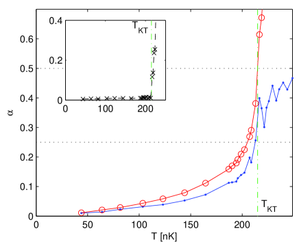
Figure 5: (color online). Comparison of two methods for determining the algebraic decay coefficient $\alpha(T)$ for the first order correlation function $g^{(1)}(\mathbf{x},\mathbf{x}^{\prime})$. The line with circle markers represents direct fits to $g^{(1)}$. These fits fail at the transition temperature as shown by the sharply diverging value of $\lvert\delta(T)\rvert$ in the inset. The filled points represent the values $\alpha^{\prime}(T)$ obtained from a simulation of the experimental analysis procedure of Hadzibabic et al. (2006), described in Sec. IV.3.2. Horizontal dotted lines at 0.25 and 0.5 correspond to the expected values of $\alpha^{\prime}$ just below and above the transition, respectively Hadzibabic et al. (2006). The vertical line is the BKT transition temperature, as estimated from the superfluid fraction calculated in Sec. IV.2.

IV.3.2 Calculation of $g^{(1)}$ via interference patterns

So far a direct probe of the in situ spatial correlations has not been possible, although important progress has been made by the NIST group Cladé et al. (2009). In the experiments of Hadzibabic et al. Hadzibabic et al. (2006) a scheme proposed by Polkovnikov et al. Polkovnikov et al. (2006) was used to infer these correlations from the “waviness” of interference patterns produced by pair of quasi-2D systems (see Sec. IV.1). In this section we simulate the experimental data analysis method, and compare inferred predictions for the correlation function against those we can directly calculate. This allows us to characterize the errors associated with this technique arising from finite size effects and finite expansion time.

To make this analysis we follow the procedure outlined in Hadzibabic et al. (2006). We fit our numerically generated interference patterns (see Sec. IV.1) to the function

$$F(x,z)=G(z)\left[1+c(x)\cos\left(\frac{2\pi z}{D}+\theta(x)\right)\right],$$ (30)

where $G(z)$ is a Gaussian envelope in the $z$-direction, $c(x)$ is the interference fringe contrast, $D$ is the fringe spacing and $\theta(x)$ is the phase of the interference pattern in the $z$-direction.

Defining the function

$$C(L_{x})=\frac{1}{L_{x}}\int_{-L_{x}/2}^{L_{x}/2}c(x)e^{i\theta(x)}dx,$$ (31)

the nature of spatial correlations is then revealed by the manner in which $\big{\langle}\lvert C(L_{x})\rvert^{2}\big{\rangle}$ decays with $L_{x}$. In particular, we identify the parameter $\alpha^{\prime}$, defined by $\big{\langle}\lvert C(L_{x})\rvert^{2}\big{\rangle}\propto L_{x}^{-2\alpha^{\prime}}$ Polkovnikov et al. (2006). For an infinite 2D system in the superfluid regime ($T<T_{\text{KT}}^{\infty}$) $\alpha^{\prime}=\alpha$ (i.e. $\alpha^{\prime}$ corresponds to the algebraic decay of correlations). For $T>T_{\text{KT}}^{\infty}$, where correlations decay exponentially, $\alpha^{\prime}$ is equal to $0.5$.

Fitting $\big{\langle}\lvert C(L_{x})\rvert^{2}\big{\rangle}$ to the algebraic decay law $AL_{x}^{\;-2\alpha^{\prime}}$ we can determine $\alpha^{\prime}$. A comparison between $\alpha^{\prime}$ inferred from the interference pattern and $\alpha$ obtained directly from $g^{(1)}$ is shown in Fig. 5. Both methods give broadly consistent predictions for $\alpha$ when $T<T_{\text{KT}}$, however our results show that there is a clear quantitative difference between the two schemes, and that $\alpha^{\prime}$ underestimates the coefficient of algebraic decay in the system (i.e. using $\alpha^{\prime}$ in Eq. (4) would overestimate the superfluid density). Near and above transition temperature, where the fits to $g^{(1)}$ fail, we observe that $\alpha^{\prime}$ converges toward $0.5$. The agreement between $\alpha$ and $\alpha^{\prime}$ in the low temperature region improves as the size of the grid is increased.

IV.4 Vortices and pairing

The simplest description of the BKT transition is that it occurs as a result of vortex pair unbinding: At $T<T_{\text{KT}}$ vortices only exist in pairs of opposite circulation, which unbind at the transition point to produce free vortices that destroy the superfluidity of the system. However, to date there are no direct experimental observations of this scenario, and theoretical studies of 2D Bose gases have been limited to qualitative inspection of the vortex distributions. In the c-field approach vortices and their dynamics are clearly revealed, unlike other ensemble-based simulation techniques where the vortices are obscured by averaging. This gives us a unique opportunity to investigate the role of vortices and pairing in a dilute Bose gas.

We detect vortices in the c-field microstates by analyzing the phase profile of the instantaneous field (see appendix C). An example of a phase profile of a field for $T<T_{\text{KT}}$ is shown in Fig. 6(a). The vortex locations reveal a pairing character, that is, the close proximity of pairs of positive (clockwise) and negative (counterclockwise) vortices relative to the average vortex separation. An important qualitative feature of our observed vortex distributions is that at high temperatures, pairing does not disappear from the system entirely. Indeed, most vortices at high temperature could be considered paired or grouped in some manner, as shown in Fig. 6(b). Perhaps this is not surprising, since positive and negative vortices have a logarithmic attraction, and we observe them to create and annihilate readily in the c-field dynamics. However, this does indicate that the use of pairing to locate the transition may be ambiguous, and we examine this aspect further below.

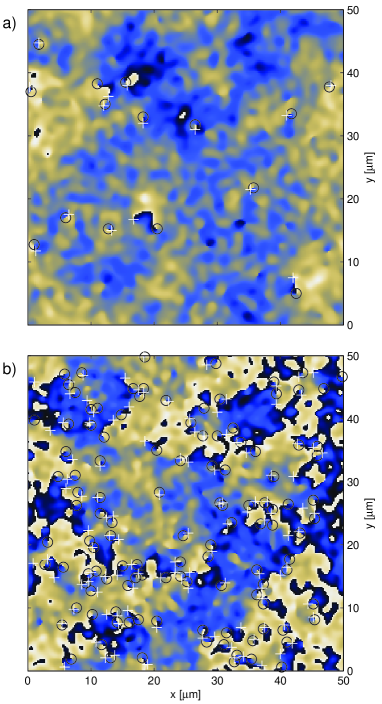
Figure 6: (color online). Phase profile of a c-field with vortices indicated. Vortices with clockwise (white $+$) and anticlockwise (black $\circ$) circulation. The phase of the classical field is indicated by shading the background between dark blue (phase 0) and light yellow (phase $2\pi$). (a) Distinctive pairing below the transition at $T=207\text{nK}\approx 0.93T_{\text{KT}}$ (b) A “vortex plasma” above the transition at $T=238\text{nK}\approx 1.07T_{\text{KT}}$.

It is also of interest to measure the number of vortices, $N_{v}$, present in the system as a function of temperature (see Fig. 7). At the lowest temperatures the system is in an ordered state, and the energetic cost of having a vortex is prohibitive. As the temperature increases there is a rapid growth of vortex population leading up to the transition point followed by linear growth above $T_{\text{KT}}$.

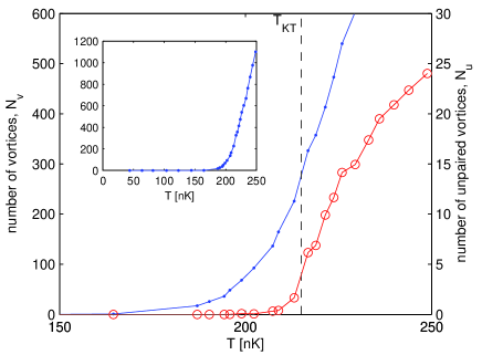
Figure 7: Total number of vortices (dots) and number of unpaired vortices (circles) as a function of temperature near the transition. While $N_{v}$ at the transition temperature is already very high, $N_{u}$ becomes nonzero only close to the transition, providing clear evidence of vortex unbinding at work. The inset shows the variation in the total number over the full temperature range of the simulations. Above the transition temperature the growth in the number of vortices becomes linear with temperature.

IV.4.1 Radial vortex density

The most obvious way to characterize vortex pairing is by defining a pair distribution function for vortices of opposite sign. Adopting the notation of Giorgetti et al. (2007), this is

$$G_{v,\pm}^{(2)}(\mathbf{r})=\left\langle\rho_{v,+}(\mathbf{0})\rho_{v,-}(\mathbf{r})\right\rangle,$$ (32)

where $\rho_{v,+}$ is the vortex density function which consists of a sum of delta-spikes,

$$\rho_{v,+}(\mathbf{r})=\sum_{i=1}^{N_{v,+}}\delta(\mathbf{r}-\mathbf{r}^{+}_{i})$$

for positive vortices at positions $\left\{\mathbf{r}^{+}_{i}\right\}$. We use the analogous definition for $\rho_{v,-}$. The associated dimensionless two-vortex correlation function is

$$g_{v,\pm}^{(2)}(\mathbf{r})=\frac{G_{v,\pm}^{(2)}(\mathbf{r})}{\langle\rho_{v,+}(\mathbf{0})\rangle\langle\rho_{v,-}(\mathbf{r})\rangle}.$$ (33)

The angular average of $g_{v,\pm}^{(2)}$ can be calculated directly from the detected vortex positions using a binning procedure on the pairwise distances $\lVert\mathbf{r}^{+}_{i}-\mathbf{r}^{-}_{j}\rVert$, and is shown in Fig. 8.

These results quantify the effect discussed earlier: Positive and negative vortices show a pairing correlation which does not disappear above $T_{\text{KT}}$. The characteristic size of this correlation, given by twice the width of the peak feature in Fig. 8, is $l_{\rm{cor}}\sim 3\mu$m (taking full width half maximum).

The shape of our pairing peak is qualitatively similar to that described in Giorgetti et al. (2007). However, in contrast to their results the width does not appear to change appreciably with temperature. Additional simulations show that increasing the interaction strength causes the peak to become squarer and wider. It is clear that while the pair size and strength revealed in $g_{v,\pm}^{(2)}({r})$ does not change appreciably as the transition is crossed, the amount of pairing relative to the background uncorrelated vortices changes considerably. This background of uncorrelated vortices is given by the horizontal plateau $g_{v,\pm}^{(2)}({r})\to 1$ at large $r$ as shown in the inset.

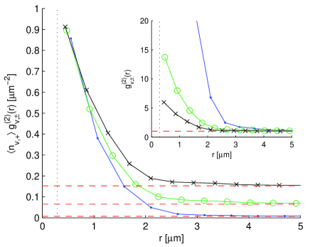
Figure 8: (color online). Angular average of the two-vortex pair distribution functions for vortices of opposite sign. Three temperatures centered about the transition are shown: dot markers $T=194$nK $\approx 0.9T_{\text{KT}}$, $f_{c}=0.34$; circle markers $T=217$nK $\approx 1.01T_{\text{KT}}$, $f_{c}=0.076$; cross markers $T=236$nK $\approx 1.1T_{\text{KT}}$, $f_{c}=0.006$. The vertical dotted line shows the value of the healing length at $T=0$. The main plot shows $g_{v,\pm}^{(2)}$ normalized by the positive vortex density; comparable magnitudes for the peaks near $r=0$ show that vortex pairing remains important over the range of temperatures studied, not only below the transition. The inset shows $g_{v,\pm}^{(2)}$ in the natural dimensionless units for which $g_{v,\pm}^{(2)}({r})\to 1$ as $r\to\infty$.

IV.4.2 Revealing unpaired vortices with coarse-graining

The function $G_{v,\pm}^{(2)}(r)$ clearly indicates the existence of vortex pairing in the system. However, it does not provide a convenient way to locate the transition temperature, since a large amount of pairing exists both below and above the transition: The expected number of neighbors for any given vortex — roughly, the area of the pairing peak of $\langle n_{v,+}\rangle G_{v,\pm}^{(2)}(r)$ shown in Fig. 8 — does not change dramatically across the transition. $\langle n_{v,+}\rangle=\langle n_{v}\rangle/2$ is the expected density of positive vortices.

We desire a quantitative observation of vortex unbinding at the transition and have therefore investigated several measures of vortex pairing . However, measures based directly on the full set of vortex positions seem to suffer from the proliferation of vortices at high temperature — an effect which tends to wash out clear signs of vortex unbinding. With this in mind, we have developed a procedure for measuring the number of unpaired vortices in our simulations, starting from the classical field rather than the full set of vortex positions.

The basis of our approach for detecting unpairing is to coarse-grain the classical field by convolution with a Gaussian filter of spatial width (standard deviation) $\sigma_{f}$. This removes all vortex pairs on length scales smaller than than $\sigma_{f}$. Figure 9 shows the count of remaining vortices as a function of filter width, along with some examples of coarse-grained fields. For $\sigma_{f}\gtrsim l_{\rm{cor}}$, the number of remaining vortices levels off and only decreases slowly with increasing $\sigma_{f}$. Ultimately the number of remaining vortices goes to zero as $\sigma_{f}\to L$.

Setting the filter width to be larger than the characteristic pairing distance, $l_{\rm{cor}}$, yields a coarse-grained field from which the pairs have been removed, but unpaired vortices remain. In our simulations we have $l_{\rm{cor}}\approx 3$ $\mu$m; we take the vortices which remain after coarse-graining with a Gaussian of standard deviation $\sigma_{f}=5$ $\mu$m to give an estimate of the number of unpaired vortices, $N_{u}$. Figure 7 shows that $N_{u}$ becomes nonzero only near the transition, in contrast to $N_{v}$ which is nonzero well below $T_{\text{KT}}$. The sharp increase in $N_{u}$ at $T_{\text{KT}}$ is a quantitative demonstration of vortex unbinding at work.

Figure 9: (color online). The coarse-graining procedure: number of vortices as a function of filter width for a temperature near the transition. The smooth curve is an average over many realizations of the field, whereas the stepped curve shows typical behavior of the number for a single field. Insets show the coarse-grained fields for various filter widths; the transformation removes vortex-antivortex pairs which are separated by approximately less than the standard deviation of the filter. In this example $N_{u}=4$ unpaired vortices remain at $\sigma_{f}=5$ $\mu$m.

In the experiment of Ref. Hadzibabic et al. (2006), the fraction of interference patterns with dislocations (e.g., see Figs. 1(c) and (d)) was measured. While isolated vortices are clearly identified by interference pattern dislocations, a lack of spatial resolution in experiments means that this type of detection method obscures the observation of tightly bound vortex pairs. The experimental resolution of 3 $\mu$m is broadly consistent with the scale of the coarse-graining filter (i.e., $\sigma_{f}=5$ $\mu$m). With this in mind, we introduce the quantity $p_{u}(T)$, defined as the probability of observing an unpaired vortex in a $50\times 50$ $\mu$m control volume at a given temperature . For the 50 $\mu$m grid we have simply $p_{u}(T)=\Pr(N_{u}\geq 1)$.

Computing $p_{u}(T)$ from our simulations yields the results shown in Fig. 10. Our results show a dramatic jump in $p_{u}$ at a temperature that is consistent with the transition temperature $T_{\text{KT}}$ determined from the superfluid fraction calculation presented in Sec. IV.2.

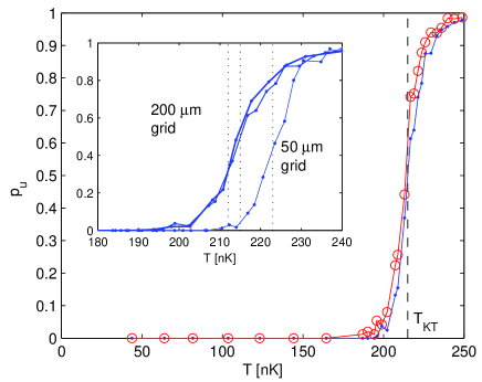
Figure 10: (color online). Comparison of vortex unpairing measures. The dots are our pairing measure based on coarse-graining the field. Circles represent the pairing as determined by the number of dislocations in the simulated interference patterns. This was the same method used in the experimental analysis of Hadzibabic et al. (2006) and coincides remarkably well with our coarse-graining based measure. Both curves are consistent with the vertical line showing the transition temperature $T_{\text{KT}}$ as determined from the superfluid fraction calculation in Sec. IV.2. The inset shows the calculated coarse-grained pairing measure for all three grid sizes, along with vertical lines showing the estimates for $T_{\text{KT}}$ derived from the superfluid fraction calculations.

From the definition, we expect that $p_{u}$ should be close to the experimentally measured frequency of dislocations. To demonstrate this relationship, we have simulated interference patterns (as described in Sec. IV.1) and detected dislocations using the experimental procedure of Ref. Hadzibabic et al. (2006): A phase gradient $d\theta/dx$ was considered to mark a dislocation whenever $\left\lvert d\theta/dx\right\rvert>\pi/4$ rad$/\mu$m. From this we can compute the probability of detecting at least one dislocation as a function of temperature. As shown in Fig. 10, the results of this procedure compare very favorably with our measure of pairing based on $p_{u}$. We note that inhomogeneous effects in experiments probably broaden the jump in $p_{u}$ appreciably compared to our homogeneous results.

V Conclusion

In this paper we have used c-field simulations of a finite-sized homogeneous system in order to investigate the physics of the 2D Bose gas in a regime corresponding to current experiments. We have directly computed the condensate and superfluid fractions as a function of temperature, and made comparisons to the superfluid fraction inferred by the first order correlation function, and using the interference scheme used in experiments. Our results for these quantities provide a quantitative test of the interference scheme for a finite system.

A beautiful possibility is the direct experimental observation of vortex-antivortex pairs, their distribution in the system, and hence a quantitative measurement of their unbinding at the BKT transition. We have calculated the vortex correlation function across the transition and provided a coarse-graining scheme for distinguishing unpaired vortices. These results suggest that the dislocations observed in experiments, due to limited optical resolution, provide an accurate measure of the unpaired vortex population and accordingly are a strong indicator of the BKT transition.

We briefly discuss the effect that harmonic confinement (present in experiments) would have on our predictions. The spatial inhomogeneity will cause the superfluid transition to be gradual, occurring first at the trap center where the density is highest, in contrast to our results where the transition occurs in the bulk. So far the superfluid fraction for the trapped system has been determined by using the universality result for the critical density in the homogeneous gas Prokof’ev and Svistunov (2002) in combination with the local density approximation Holzmann and Krauth (2008); Bisset et al. (2009). It would be interesting to be able to compute the superfluid fraction independently as we have done here; however it is not clear how to do so.

Bisset et al. Bisset et al. (2009) used an extension of the c-field method for the trapped 2D gas to examine $g^{(1)}$ and found similar results for the onset of algebraic decay of correlations at the transition. Their analysis was restricted to the small region near the trap center where the density is approximately constant; we expect the results of our vortex correlation function and the coarse-graining scheme should similarly be applicable to the trapped system in the central region. Except in very weak traps, the size of this region is relatively small and will likely prove challenging to measure experimentally.

Our results for the homogeneous gas emphasize the clarity with which ab initio theoretical methods can calculate quantities directly observable in experiments, such as interference patterns. This should allow direct comparisons with experiments, providing stringent tests of many-body theory.

Appendix A Simulation using the PGPE

Here we outline our procedure for determining the properties of the C region and the steps used to create initial states for the PGPE solver. The C region itself is characterized by the cutoff momentum $K$, while the initial states are characterized by the energy $E_{\text{\bf{C}}}$ and number $N_{\text{\bf{C}}}$. We want to obtain values of these three properties which are consistent with a specified temperature $T$ and total number of atoms $N$.

A.1 Hartree-Fock-Bogoliubov analysis

To generate an initial estimate of the C region parameters we solve the self-consistent Hartree-Fock-Bogoliubov (HFB) equations in the so-called Popov approximation Griffin (1996) to find an approximate thermal state for the system at a temperature $T$. The resulting state is a Bose Einstein distribution of quasiparticles interacting only via the mean-field, expressed in terms of the quasiparticle amplitudes $u_{\mathbf{k}}$ and $v_{\mathbf{k}}$.

Occupations for the C region field may be computed directly from the quasiparticle occupations via

$$n_{\mathbf{k}}=\left(u_{\mathbf{k}}^{2}+v_{\mathbf{k}}^{2}\right)N_{B}(E_{\mathbf{k}})+v_{\mathbf{k}}^{2},$$ (34)

where $N_{B}$ is the Bose Einstein distribution and $E_{\mathbf{k}}$ is the quasiparticle energy which is obtained by solving the Bogoliubov-de Gennes equations self consistently  Griffin (1996). This allows us to compute the cutoff as the maximum value of $\lVert\mathbf{k}\rVert$ consistent with sufficient modal occupation:

$$K=\max\{\lVert\mathbf{k}\rVert\colon n_{\mathbf{k}}\geq n_{\text{cut}}\}.$$ (35)

We choose $n_{\text{cut}}=5$ for the sufficient occupation condition on the C region modes.

The number of atoms below the cutoff may be computed directly from the sum of the condensate number $N_{0}$ and the number of C region excited state atoms, $N_{1\text{\bf{C}}}$:

$$N_{\text{\bf{C}}}=N_{0}+N_{1\text{\bf{C}}},\quad\text{where}\quad N_{1\text{\bf{C}}}=\sum_{\mathbf{k}\in\text{\bf{C}}\backslash\{\mathbf{0}\}}n_{\mathbf{k}}.$$ (36)

For the total energy below the cutoff, we use the expression

$$E_{\text{\bf{C}}}=\frac{\hbar^{2}}{mL^{2}}\left(\frac{gN_{0}^{2}}{2}+\lambda N_{1\text{\bf{C}}}-gN_{1\text{\bf{C}}}^{2}\right)\\ +\sum_{\mathbf{k}\in\text{\bf{C}}\backslash\{\mathbf{0}\}}E_{\mathbf{k}}\left[N_{B}(E_{\mathbf{k}})-v_{\mathbf{k}}^{2}\right]$$ (37)

where $\lambda=g(N_{0}+2N_{1\text{\bf{C}}})$. Rearranging, this is

$$E_{\text{\bf{C}}}=\frac{\hbar^{2}g}{2mL^{2}}\left(N_{\text{\bf{C}}}^{2}+N_{1\text{\bf{C}}}^{2}\right)+\sum_{\mathbf{k}\in\text{\bf{C}}\backslash\{\mathbf{0}\}}E_{\mathbf{k}}\left[N_{B}(E_{\mathbf{k}})-v_{\mathbf{k}}^{2}\right].$$ (38)

The expression (38) differs from Eq. (22) of Griffin (1996) as we have retained the zeroth order (constant) terms that are required to match the energy scale of the HFB analysis to the zero point of energy in the classical field simulations.

A.2 Initial conditions for fixed total number

A simple comparison between simulations at varying temperatures can only be carried out if the total number of atoms is fixed. This presents a problem in our simulations: although the number of atoms and energy of the C region can be directly specified (see Sec. A.3), we may only determine the total number after performing a simulation. This is because the number of atoms in the I region depends on the temperature and chemical potential which are calculated by ergodic averaging of the C region simulations.

Formally, this may be stated as a root-finding problem: solve

$$N(N_{\text{\bf{C}}},E_{\text{\bf{C}}})=N_{\text{tot}}$$ (39)

with initial guess provided by the solution to the HFB analysis in Sec. A.1. Although both $N_{\text{\bf{C}}}$ and $E_{\text{\bf{C}}}$ affect the total number $N$, we choose to fix $N_{\text{\bf{C}}}$ to the initial guess and to vary $E_{\text{\bf{C}}}$ until the desired total number is found.

We note that evaluating the function $N(N_{\text{\bf{C}}},E_{\text{\bf{C}}})$ is very computationally expensive and difficult to fully automate since it involves a simulation and several steps of analysis. For this reason we use a nonstandard root finding procedure: For the first iteration we simulate three energies about the initial guess $E_{\text{\bf{C}}}$ such that the results crudely span $N_{\text{tot}}$; these three simulations can be performed in parallel which significantly reduces the time to a solution. A second guess was obtained by quadratic fitting of $E_{\text{\bf{C}}}$ as a function of $N$ which gives $N$ accurate to within about 5% of $N_{\text{tot}}$. An addition iteration using the same interpolation method takes $N$ to within 0.3%, which we consider sufficient.

We note that changing $E_{\text{\bf{C}}}$ during the root finding procedure means we have no direct control over the final temperature of each specific simulation. In our case this is not a problem because we only require a range of temperatures spanning the transition. In principle one could solve for a given temperature by allowing $N_{\text{\bf{C}}}$ to vary in addition to $E_{\text{\bf{C}}}$.

A.3 Initial conditions for given $E_{\text{\bf{C}}}$ and $N_{\text{\bf{C}}}$

We compute initial conditions for the C region field in a similar way to Davis et al. (2002). Using the representation for the C region given by Eq. (10), the task is to choose appropriate values for the $\{c_{\mathbf{n}}\}$. As a first approximation, choose the smallest value for a momentum cutoff $K^{\prime}$ such that the field with coefficients

$$c_{\mathbf{n}}=\begin{cases}Ae^{i\theta_{\mathbf{n}}}\qquad&\text{for }0<\lVert\mathbf{k}\rVert\leq K^{\prime},\\ 0\qquad&\text{for }\lvert\mathbf{k}\rvert>K^{\prime},\end{cases}$$ (40)

has energy greater than $E_{\text{\bf{C}}}$. Here $A$ is chosen so that the field has normalization corresponding to $N_{\text{\bf{C}}}$ atoms, and $\theta_{\mathbf{n}}$ is a randomly chosen phase which is fixed for each mode at the start of the procedure. The random phases allow us to generate many unique random initial states at the same energy.

By definition, the field defined by (40) has energy slightly above the desired energy. This problem is solved by mixing it with the lowest energy state:

$$c_{\mathbf{n}}=\begin{cases}A^{\prime}e^{i\theta_{\mathbf{0}}}\qquad&\text{for }\mathbf{n}=\mathbf{0},\\ 0\qquad&\text{elsewhere},\end{cases}$$ (41)

using a root finding procedure to converge on the desired energy $E_{\text{\bf{C}}}$. The scheme generates random realizations of a non-equilibrium field with given $E_{\text{\bf{C}}}$ and $N_{\text{\bf{C}}}$ which are then simulated to equilibrium before using ergodic averaging for computing statistics.

Appendix B I region integrals

Our assumed self-consistent Wigner function (Sec. III.2) for the I region atoms takes a particularly simple form in the homogeneous case:

$$W(\mathbf{k},\mathbf{x})=\frac{1}{(2\pi)^{2}}\frac{1}{e^{(\hbar^{2}\mathbf{k}^{2}/2m+2\hbar^{2}gn_{\text{\bf{C}}}/m-\mu_{\text{\bf{C}}})/k_{B}T}-1}.$$ (42)

The above-cutoff density may then be found by direct integration:

$$n_{\text{\bf{I}}}(\mathbf{x}) =\int_{\lVert\mathbf{k}\rVert\geq K}d^{2}\mathbf{k}\;W_{\text{\bf{I}}}(\mathbf{k},\mathbf{x}),$$ (43)

$$=-\frac{1}{\lambda^{2}}\ln\left[1-e^{-(\hbar^{2}K^{2}/2m+2\hbar^{2}gn_{\text{\bf{C}}}/m-\mu_{\text{\bf{C}}})/k_{B}T}\right],$$ (44)

with $\lambda$ the thermal de Broglie wavelength.

In a similar way, the assumed Wigner function allows any desired physical quantity to be estimated via a suitable integral. A particular quantity of interest in the current work is the first order correlation function, which can be obtained from the Wigner function as Naraschewski and Glauber (1999)

$$G^{(1)}_{\text{\bf{I}}}(\mathbf{x},\mathbf{x}^{\prime})=\int_{\lVert\mathbf{k}\rVert\geq K}d^{2}\mathbf{k}\;e^{-i\mathbf{k}\cdot(\mathbf{x}-\mathbf{x}^{\prime})}\;W_{\text{\bf{I}}}\big{(}\mathbf{k},\tfrac{\mathbf{x}+\mathbf{x}^{\prime}}{2}\big{)}.$$ (45)

This integral is of the general form

$$I_{1}(\mathbf{r}):=\int_{\lVert\mathbf{k}\rVert>K}d^{2}\mathbf{k}\;\frac{e^{-i\mathbf{k}\cdot\mathbf{r}}}{e^{A\mathbf{k}^{2}+B}-1},$$ (46)

for constants $A$ and $B$. Noting that $I_{1}$ depends only on the length, $r$ of $\lVert\mathbf{r}\rVert$, and transforming $k$ to polar coordinates $(\kappa,\theta)$, we have

$$I_{1}(\mathbf{r}) =\int_{K}^{\infty}d\kappa\frac{\kappa}{e^{A\kappa^{2}+B}-1}\int_{0}^{2\pi}d\theta\;e^{-ir\kappa\cos\theta},$$ (47)

$$=\int_{K}^{\infty}d\kappa\frac{\kappa}{e^{A\kappa^{2}+B}-1}\,2\left[\Gamma(\tfrac{1}{2})\right]^{2}J_{0}(r\kappa),$$ (48)

(see (Gradshteyn and Ryzhik, 2000, p902) for the Bessel function identity).

Thus we obtain $G_{\text{\bf{I}}}^{(1)}(\mathbf{x},\mathbf{x}^{\prime})$ in terms of a one dimensional integral which may be performed numerically:

$$G_{\text{\bf{I}}}^{(1)}(\mathbf{x},\mathbf{x}^{\prime})=\frac{1}{2\pi}\int_{K}^{\infty}d\kappa\;\frac{\kappa J_{0}(\kappa\lVert\mathbf{x}-\mathbf{x}^{\prime}\rVert)}{e^{(\hbar^{2}\kappa^{2}/2m+2\hbar^{2}gn_{\text{\bf{C}}}/m-\mu_{\text{\bf{C}}})/k_{B}T}-1}.$$ (49)

Appendix C Vortex detection

The defining feature of a “charge-$m$” vortex is that the phase $\theta$ of the complex field $\psi(\mathbf{x})=\lvert\psi{(\mathbf{x})}\rvert e^{i\theta(\mathbf{x})}$ changes continuously from $0$ to $2m\pi$ around any closed curve which circles the vortex core. We express our field $\psi$ on a discrete grid in position space; the aim of vortex detection is then to determine which grid plaquettes (that is, sets of four adjacent grid points) contain vortex cores.

To obtain the phase winding about a plaquette, first consider the phase at two neighboring grid points A and B. We are interested in the unwrapped phase difference $\Delta\theta_{\text{AB}}$ between the grid points; unwrapping ensures that the phase is continuous between A and B. (In the discrete setting such continuity is poorly defined; the best we can do is to correct for the possibility of $2\pi$ phase jumps by adding or subtracting factors of $2\pi$ so that $\left\lvert\Delta\theta_{\text{AB}}\right\rvert<\pi$.) The unwrapped phase differences around a grid plaquette tell us a total phase change $\theta_{\text{wrap}}=\sum_{i}\Delta\theta_{i,i+1}=2m\pi$ where $m\in\mathbb{Z}$ is the winding number or “topological charge”.

Due to the necessity of unwrapping the phase, a four-point grid plaquette cannot unambiguously support vortices with charge larger than one. Luckily, such vortices are energetically unfavorable in 2D Bose gases (Pitaevskii and Stringari, 2003, p.83) so we need only concern ourselves with detecting vortices with winding number $\pm 1$ in this work. The positions obtained from a given run of our vortex detection algorithm are the labeled $\{\mathbf{r}^{+}_{i}\}$ and $\{\mathbf{r}^{-}_{i}\}$ for winding numbers $+1$ and $-1$, respectively.

Appendix D Superfluid fraction

One of the important characteristics of the BKT transition is the presence of superfluidity, even in the absence of conventional long range order. In the following we describe a method to calculate the superfluid fraction from our classical field description. The method is attractive because it makes use of momentum correlations which may be extracted directly from our equilibrium simulations without any need to introduce additional boundary conditions or moving defects.

D.1 Superfluid fraction via momentum density correlations

Our derivation is based on the procedure presented in (Forster, 1975, p.214), (see also Baym (1969) and (Pitaevskii and Stringari, 2003, p.96)). The central idea is to establish a relationship between i) the autocorrelations of the momentum density in the simulated ensemble and ii) the linear response of the fluid to slowly moving boundaries; (i) is a quantity we can calculate, while (ii) is related to the basic properties of a superfluid via a simple thought experiment.

To connect the macroscopic, phenomenological description of superfluidity with our microscopic theory, we make use of the thought experiment shown schematically in Fig. 11(b): Consider an infinitely long box, $B$ containing superfluid, and accelerate the box along its long axis until it reaches a small velocity $\mathbf{u}$. Due to viscous interactions with the walls, such a box filled with a normal fluid should have a momentum density at equilibrium of $\langle\hat{\mathbf{p}}\rangle_{\mathbf{u}}=n\mathbf{u}$. The notation $\langle\cdot\rangle_{\mathbf{u}}$ denotes an expectation value in the ensemble with walls moving with velocity $\mathbf{u}$.

Because superfluids are nonviscous, the observed value for the momentum density in a superfluid is less than the value $n\mathbf{u}$ expected for a classical fluid. In Landau’s two-fluid model we attribute the observed momentum density, $\rho_{n}\mathbf{u}$, to the “normal fraction” where $\rho_{n}$ is the normal fluid density. The superfluid fraction remains stationary in the lab frame, even at equilibrium and makes up the remaining mass with density $\rho_{s}=n-\rho_{n}$.

In order to apply the usual procedures of statistical mechanics to the thought experiment, we consider two frames: the “lab frame” in which the walls move with velocity $\mathbf{u}$ in the $x$-direction and the “wall frame” in which the walls are at rest.

\psfrag{velu}{$\mathbf{u}$}\psfrag{limy}{$\displaystyle\lim_{L_{y}\to\infty}$}\psfrag{limx}{$\displaystyle\lim_{L_{x}\to\infty}$}\psfrag{superflui}{Superfluid}\psfrag{Ly}{$L_{y}$}\psfrag{Lx}{$L_{x}$}\psfrag{aa}{a)}\psfrag{bb}{b)}\psfrag{cc}{c)}\psfrag{dd}{d)}\includegraphics[width=227.62204pt]{fig11.eps}

Figure 11: Thought experiment used in deriving the superfluid density. The walls move with velocity $\mathbf{u}$ in the $x$ direction. To begin with, we imagine that the superfluid sits in a box of dimensions $L_{x}\times L_{y}$ as shown in a). We later take the limit as the box walls recede to infinity to get the thermodynamic limit d). The order of the limits is critically important: the path b) leads to superflow while the path c) results in the entire fluid moving along with the walls.

Assuming that the fluid is in thermal equilibrium with the walls, the density matrix in the grand canonical ensemble is given by the usual expression $\hat{\rho}=e^{-\beta(H_{\mathbf{u}}-\mu N)}/\operatorname{Tr}\left(e^{-\beta(H_{\mathbf{u}}-\mu N)}\right)$ where $H_{\mathbf{u}}$ is the Hamiltonian of the system in the wall frame and $\beta=1/k_{B}T$. A Galilean transformation relates $H_{\mathbf{u}}$ to the Hamiltonian in the lab frame, $H_{\mathbf{u}}=H-\mathbf{u}\cdot\hat{\mathbf{P}}+\frac{1}{2}Mu^{2}$, where $\hat{\mathbf{P}}=\int_{B}\hat{\mathbf{p}}(\mathbf{x})d^{2}r$ is the total momentum, $M=mN$ is the total mass and $\hat{\mathbf{p}}(\mathbf{x})$ is the momentum density operator at point $\mathbf{x}$. The expectation value for the momentum density in the presence of moving walls is then given by the expression

$$\left\langle\hat{\mathbf{p}}(\mathbf{x})\right\rangle_{\mathbf{u}} =\operatorname{Tr}[\hat{\rho}\,\hat{\mathbf{p}}(\mathbf{x})],$$ (50)

$$=\frac{\operatorname{Tr}\big{(}e^{-\beta(H-\hat{\mathbf{P}}\cdot\mathbf{u}+(mu^{2}/2-\mu)N)}\hat{\mathbf{p}}(\mathbf{x})\big{)}}{\operatorname{Tr}\big{(}e^{-\beta(H-\hat{\mathbf{P}}\cdot\mathbf{u}+(mu^{2}/2-\mu)N}\big{)}}.$$ (51)

Expanding this expression to first order in $\mathbf{u}$ yields

$$\left\langle\hat{\mathbf{p}}(\mathbf{x})\right\rangle_{\mathbf{u}}=\left\langle\hat{\mathbf{p}}(\mathbf{x})\right\rangle+\beta\big{(}\langle\hat{\mathbf{p}}(\mathbf{x})\hat{\mathbf{P}}\cdot\mathbf{u}\rangle-\left\langle\hat{\mathbf{p}}(\mathbf{x})\right\rangle\langle\hat{\mathbf{P}}\cdot\mathbf{u}\rangle\big{)},$$ (52)

where all the expectation values on the right hand side are now taken in the equilibrium ensemble with the walls at rest. Since $\langle\hat{\mathbf{p}}(\mathbf{x})\rangle=0$ in our equilibrium ensemble, this simplifies to

$$\left\langle\hat{\mathbf{p}}(\mathbf{x})\right\rangle_{\mathbf{u}} =\beta\big{\langle}\hat{\mathbf{p}}(\mathbf{x})\hat{\mathbf{P}}\big{\rangle}\cdot\mathbf{u},$$ (53)

$$=\beta\int_{B}d^{2}\mathbf{x}^{\prime}\,\left\langle\hat{\mathbf{p}}(\mathbf{x})\hat{\mathbf{p}}(\mathbf{x}^{\prime})\right\rangle\cdot\mathbf{u},$$ (54)

where $\hat{\mathbf{p}}(\mathbf{x})\hat{\mathbf{p}}(\mathbf{x}^{\prime})$ is a dyad [i.e., a rank-two tensor; the outer product of $\hat{\mathbf{p}}(\mathbf{x})$ and $\hat{\mathbf{p}}(\mathbf{x}^{\prime})$].

To make further progress, we wish to take the limit as the system gets very large (write “$B\to\infty$”). To this end, we first consider some properties of the correlation functions in the infinite system. The infinite system is homogeneous, which implies that $\left\langle\hat{\mathbf{p}}(\mathbf{x})\hat{\mathbf{p}}(\mathbf{x}^{\prime})\right\rangle_{\infty}=\left\langle\hat{\mathbf{p}}(\mathbf{x}+\mathbf{r})\hat{\mathbf{p}}(\mathbf{x}^{\prime}+\mathbf{r})\right\rangle_{\infty}$ for any $\mathbf{r}$, where $\left\langle\cdot\right\rangle_{\infty}$ indicates an average in the infinite system. As a consequence, we may express the correlations — in the infinite system — in terms of the Fourier transform in the relative coordinate $\mathbf{x}^{\prime}-\mathbf{x}$:

$$\left\langle\hat{\mathbf{p}}(\mathbf{x})\hat{\mathbf{p}}(\mathbf{x}^{\prime})\right\rangle_{\infty} =\left\langle\hat{\mathbf{p}}(\mathbf{0})\hat{\mathbf{p}}(\mathbf{x}^{\prime}-\mathbf{x})\right\rangle_{\infty},$$ (55)

$$=\frac{1}{(2\pi)^{2}}\int d^{2}\mathbf{k}\,e^{i\mathbf{k}\cdot(\mathbf{x}^{\prime}-\mathbf{x})}\chi(\mathbf{k}),$$ (56)

where all the important features of the correlations are now captured by the tensor

$$\chi(\mathbf{k})=\int d^{2}\mathbf{r}\,e^{-i\mathbf{k}\cdot\mathbf{r}}\left\langle\hat{\mathbf{p}}(\mathbf{0})\hat{\mathbf{p}}(\mathbf{r})\right\rangle_{\infty}.$$ (57)

Because of the isotropy of the fluid in the infinite system, $\chi(\mathbf{k})$ obeys the transformation law $\chi(O\mathbf{k})=O^{-1}\chi(\mathbf{k})O$ for any $2\times 2$ orthogonal matrix $O$. This implies that $\chi$ may be decomposed into the sum of longitudinal and transverse parts:

$$\chi(\mathbf{k})=\tilde{\mathbf{k}}\tilde{\mathbf{k}}\chi_{l}(k)+\big{(}I-\tilde{\mathbf{k}}\tilde{\mathbf{k}}\big{)}\chi_{t}(k)$$ (58)

where $\tilde{\mathbf{k}}=\mathbf{k}/k$, $k=\lVert\mathbf{k}\rVert$ and $I$ is the identity. The transverse and longitudinal functions $\chi_{t}$ and $\chi_{l}$ are scalars which depend only on the length $k$.

We now return our attention to the finite system. If the finite box $B$ is large then the momentum correlations in the bulk will be very similar to the values for the infinite system. Therefore, when $\mathbf{x}$ and $\mathbf{x}^{\prime}$ are far from the boundaries, we may approximate

$$\left\langle\hat{\mathbf{p}}(\mathbf{x})\hat{\mathbf{p}}(\mathbf{x}^{\prime})\right\rangle \approx\left\langle\hat{\mathbf{p}}(\mathbf{x})\hat{\mathbf{p}}(\mathbf{x}^{\prime})\right\rangle_{\infty}$$ (59)

$$=\frac{1}{(2\pi)^{2}}\int d^{2}\mathbf{k}\,e^{i\mathbf{k}\cdot(\mathbf{x}^{\prime}-\mathbf{x})}\chi(\mathbf{k})$$ (60)

which in combination with Eq. (54) yields

$$\left\langle\hat{\mathbf{p}}(\mathbf{x})\right\rangle_{\mathbf{u}} \approx\beta\int_{B}d^{2}\mathbf{x}^{\prime}\frac{1}{(2\pi)^{2}}\int d^{2}\mathbf{k}\,e^{i\mathbf{k}\cdot(\mathbf{x}^{\prime}-\mathbf{x})}\chi(\mathbf{k})\cdot\mathbf{u}$$ (61)

$$=\beta\int d^{2}\mathbf{k}\,\Delta_{B}(\mathbf{k})e^{i\mathbf{k}\cdot\mathbf{x}}\chi(\mathbf{k})\cdot\mathbf{u}.$$ (62)

Here we have defined the nascent delta function $\Delta_{B}(\mathbf{k}):=\frac{1}{(2\pi)^{2}}\int_{B}d^{2}\mathbf{x}^{\prime}\,e^{i\mathbf{k}\cdot\mathbf{x}^{\prime}}$ which has the property $\Delta_{B}(\mathbf{k})\to\delta(\mathbf{k})$ as $B\to\infty$.

We are now in a position to carry out the limiting procedure to increase the box size to infinity. However, care must be taken because the simple expression $\lim_{B\to\infty}\left\langle\hat{\mathbf{p}}(\mathbf{x})\right\rangle_{\mathbf{u}}$ is not well defined without further qualification of the limiting process $B\to\infty$.

To resolve this subtlety we must insert a final vital piece of physical reasoning. Let us assume for simplicity that $\mathbf{u}$ is directed along the $x$-direction, and the box $B$ is aligned with the $x$ and $y$ axes with dimensions $L_{x}{\times}L_{y}$. As shown in Fig. 11, there are two possibilities for taking the limits, representing different physical situations.

On the one hand [Fig. 11(b)], we may take the limit $L_{x}\to\infty$ first, which gives us an infinitely long channel in which superfluid can remain stationary while only the normal fraction moves with the walls in the $x$-direction. We have

$$\rho_{n}\mathbf{u} =\lim_{L_{y}\to\infty}\lim_{L_{x}\to\infty}\left\langle\hat{\mathbf{p}}(\mathbf{x})\right\rangle_{\mathbf{u}}$$ (63)

$$=\lim_{L_{y}\to\infty}\lim_{L_{x}\to\infty}\beta\int d^{2}\mathbf{k}\,\Delta_{B}(\mathbf{k})e^{i\mathbf{k}\cdot\mathbf{x}}\chi(\mathbf{k})\cdot\mathbf{u}$$ (64)

$$=\beta\lim_{k_{y}\to 0}\lim_{k_{x}\to 0}\chi(\mathbf{k})\cdot\mathbf{u}$$ (65)

where we use the fact that $\Delta_{B}(\mathbf{k})$ can be decomposed into the product $\Delta_{L_{x}}(k_{x})\Delta_{L_{y}}(k_{y})$ with $\Delta_{L}(k)\to\delta(k)$ as $L\to\infty$. Employing the decomposition of $\chi$ given in Eq. (58) allows the density of the normal fraction to be related to the transverse component of $\chi$ evaluated at zero:

$$\rho_{n}=\beta\lim_{k\to 0}\chi_{t}(k)=\beta\chi_{t}(0).$$ (66)

On the other hand [Fig. 11(c)] we may take the limit $L_{y}\to\infty$ first, resulting in an infinitely long channel — with velocity perpendicular to the walls — in which the entire body of the fluid must move regardless of the superfluidity. In a similar way to the previous paragraph, $n\mathbf{u}=\beta\lim_{k_{x}\to\mathbf{0}}\lim_{k_{y}\to\mathbf{0}}\chi(\mathbf{k})\cdot\mathbf{u}$, and making use of the decomposition in Eq. (58), the total density is related to the longitudinal component of the correlations:

$$n=\beta\lim_{k\to 0}\chi_{l}(k)=\beta\chi_{l}(0).$$ (67)

With these expressions, the normal fraction $f_{n}$ may finally be expressed directly as

$$f_{n}=\rho_{n}/n=\lim_{k\to 0}\chi_{t}(k)/\lim_{k\to 0}\chi_{l}(k)$$ (68)

while the superfluid fraction is $f_{s}=1-f_{n}$. Thus, we have expressed the superfluid and normal fractions in terms of a correlation function which can be directly computed from our simulation results.

D.2 Numerical procedure

To determine the superfluid fraction for our system, we need to estimate the tensor of momentum density correlations $\chi$ from the simulation results. For our finite system constrained to a periodic simulation box, we may compute the momentum correlations only at discrete grid points. The discrete analogue of Eq. (57) leads to the expression

$$\chi(\mathbf{k})\propto\left\langle\mathbf{p}_{\mathbf{k}}\mathbf{p}_{-\mathbf{k}}\right\rangle$$ (69)

where the constant of proportionality is not important to the final result, and $\mathbf{p}_{\mathbf{k}}$ are the discrete Fourier coefficients of $\mathbf{p}(\mathbf{x})$ over our simulation box.

The momentum density operator is given by

$$\hat{\mathbf{p}}(\mathbf{x})=\frac{i\hbar}{2}\left[(\nabla\hat{\psi}^{\dagger}(\mathbf{x}))\hat{\psi}(\mathbf{x})-\hat{\psi}^{\dagger}(\mathbf{x})\nabla\hat{\psi}(\mathbf{x})\right]$$ (70)

which may be derived by considering the continuity equation for the number density, $\big{\langle}\hat{\psi}^{\dagger}(\mathbf{x})\hat{\psi}(\mathbf{x})\big{\rangle}$. For a given classical field Eq. (10), the Fourier coefficients of $\mathbf{p}$ may be written as

$$\mathbf{p}_{\mathbf{k}}=\frac{\hbar}{2\sqrt{A_{B}}}\sum_{\mathbf{k}^{\prime}}(2\mathbf{k}^{\prime}+\mathbf{k})c^{*}_{\mathbf{k}^{\prime}}c_{\mathbf{k}+\mathbf{k}^{\prime}},$$ (71)

where $A_{B}$ is the area of the system. Computing a value for all $\mathbf{p}_{\mathbf{k}}$ at each time step, we then evaluate $\chi(\mathbf{k})$ via the usual ergodic averaging procedure using Eq. (69).

Having evaluated $\chi(\mathbf{k})$, we are left with performing the decomposition into longitudinal and transverse parts. For this, simply note that Eq. (58) implies $\chi_{l}(k)=\tilde{\mathbf{k}}\cdot\chi(\mathbf{k})\cdot\tilde{\mathbf{k}}$, and $\chi_{t}(k)=\tilde{\mathbf{w}}\cdot\chi(\mathbf{k})\cdot\tilde{\mathbf{w}}$, where $\tilde{\mathbf{w}}$ is a unit vector perpendicular to $\tilde{\mathbf{k}}$.

Values for $\chi_{t}$ and $\chi_{l}$ may be collected for all angles as a function of $k$, and a fitting procedure used to perform the extrapolation $k\to 0$; this procedure is illustrated in Fig. 12. At low temperatures, the extrapolation is quite reliable, but becomes more difficult near the transition where sampling noise increases and $\chi_{t}(k)$ changes rapidly near $k=0$. Without a known functional form, we settled for a quadratic weighted least squares fit of $\ln(\chi_{t})$ and $\ln(\chi_{l})$ versus $k$. A weighting of $1/k$ was used to counteract the fact that the density of samples of $\chi$ vs $k$ scales proportionally with $k$ due to the square grid on which $\chi(\mathbf{k})$ is evaluated. The logarithm was used to improve the fits of $\chi_{t}$ very near the transition where it varies non-quadratically near $k=0$. The fitting procedure and extrapolation to $k=0$ generally produces reasonable results, but is somewhat sensitive to numerical noise. For this reason, the computed superfluid fraction at high temperatures is not exactly zero (see Fig. 2).

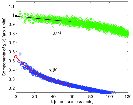
Figure 12: (color online). Example fitting and extrapolation to $k=0$ for the transverse and longitudinal components of the momentum density autocorrelation tensor, $\chi$. The apparent functional form for $\chi_{t}$ and $\chi_{l}$ changes with temperature — particularly near the transition — which along with the sampling noise makes them difficult to fit reliably. The data shown corresponds to a temperature slightly below the transition.

References

- Mermin and Wagner (1966) N. D. Mermin and H. Wagner, Phys. Rev. Lett. 17, 1133 (1966).
- Hohenberg (1967) P. C. Hohenberg, Physical Review 158, 383 (1967).
- Berezinskii (1971) V. L. Berezinskii, Sov. Phys. JETP 32, 493 (1971).
- Kosterlitz and Thouless (1973) J. M. Kosterlitz and D. J. Thouless, J. Phys. C 6, 1181 (1973).
- Posazhennikova (2006) A. Posazhennikova, Rev. Mod. Phys. 78, 1111 (2006).
- Bishop and Reppy (1978) D. J. Bishop and J. D. Reppy, Phys. Rev. Lett. 40, 1727 (1978).
- Stock et al. (2005) S. Stock, Z. Hadzibabic, B. Battelier, M. Cheneau, and J. Dalibard, Phys. Rev. Lett. 95, 190403 (2005).
- Hadzibabic et al. (2006) Z. Hadzibabic, P. Kruger, M. Cheneau, B. Battelier, and J. Dalibard, Nature 441, 1118 (2006).
- Krüger et al. (2007) P. Krüger, Z. Hadzibabic, and J. Dalibard, Phys. Rev. Lett. 99, 040402 (2007).
- Schweikhard et al. (2007) V. Schweikhard, S. Tung, and E. A. Cornell, Phys. Rev. Lett. 99, 030401 (2007).
- Cladé et al. (2009) P. Cladé, C. Ryu, A. Ramanathan, K. Helmerson, and W. D. Phillips, Phys. Rev. Lett. 102, 170401 (2009).
- Görlitz et al. (2001) A. Görlitz, J. M. Vogels, A. E. Leanhardt, C. Raman, T. L. Gustavson, J. R. Abo-Shaeer, A. P. Chikkatur, S. Gupta, S. Inouye, T. Rosenband, et al., Phys. Rev. Lett. 87, 130402 (2001).
- Smith et al. (2005) N. L. Smith, W. H. Heathcote, G. Hechenblaikner, E. Nugent, and C. J. Foot, J. Phys. B 35, 223 (2005).
- Prokof’ev et al. (2001) N. Prokof’ev, O. Ruebenacker, and B. Svistunov, Phys. Rev. Lett. 87, 270402 (2001).
- Prokof’ev and Svistunov (2002) N. Prokof’ev and B. Svistunov, Phys. Rev. A 66, 043608 (2002).
- Bisset and Blakie (2009) R. N. Bisset and P. B. Blakie, Phys. Rev. A 80, 045603 (2009).
- Mathey and Polkovnikov (2009) L. Mathey and A. Polkovnikov, Phys. Rev. A 80, 041601 (2009).
- Sato et al. (2009) T. Sato, T. Suzuki, and N. Kawashima, J. Phys. Conf. Ser. 150, 032094 (2009).
- Gies and Hutchinson (2004) C. Gies and D. A. W. Hutchinson, Phys. Rev. A 70, 043606 (2004).
- Schumayer and Hutchinson (2007) D. Schumayer and D. A. W. Hutchinson, Phys. Rev. A 75, 015601 (2007).
- Holzmann and Krauth (2008) M. Holzmann and W. Krauth, Phys. Rev. Lett. 100, 190402 (2008).
- Holzmann et al. (2009) M. Holzmann, M. Chevallier, and W. Krauth, arxiv preprint arXiv:0911.1704 (2009).
- Simula and Blakie (2006) T. P. Simula and P. B. Blakie, Phys. Rev. Lett. 96, 020404 (2006).
- Simula et al. (2008) T. P. Simula, M. J. Davis, and P. B. Blakie, Phys. Rev. A 77, 023618 (2008).
- Bisset et al. (2009) R. N. Bisset, M. J. Davis, T. P. Simula, and P. B. Blakie, Phys. Rev. A 79, 033626 (2009).
- Giorgetti et al. (2007) L. Giorgetti, I. Carusotto, and Y. Castin, Phys. Rev. A 76, 013613 (2007).
- Petrov et al. (2000) D. S. Petrov, M. Holzmann, and G. V. Shlyapnikov, Phys. Rev. Lett. 84, 2551 (2000).
- Chaikin and Lubensky (1995) P. M. Chaikin and T. C. Lubensky, Principles of Condensed Matter Physics (Cambridge University press, Cambridge, 1995).
- Nelson and Kosterlitz (1977) D. R. Nelson and J. M. Kosterlitz, Phys. Rev. Lett. 39, 1201 (1977).
- Popov (1983) V. Popov, Functional Integrals in Quantum Field Theory and Statistical Physics (Reidel, Dordrecht, 1983).
- Kagan et al. (1987) Y. Kagan, B. V. Svistunov, and G. V. Shlyapnikov, Sov. Phys. JETP 66, 314 (1987).
- Fisher and Hohenberg (1988) D. S. Fisher and P. C. Hohenberg, Phys. Rev. B 37, 4936 (1988).
- Blakie et al. (2008) P. B. Blakie, A. S. Bradley, M. J. Davis, R. J. Ballagh, and C. W. Gardiner, Adv. Phys. 57, 363 (2008).
- Kashurnikov et al. (2001) V. A. Kashurnikov, N. V. Prokof’ev, and B. V. Svistunov, Phys. Rev. Lett. 87, 120402 (2001).
- Davis et al. (2001a) M. J. Davis, R. J. Ballagh, and K. Burnett, J. Phys. B 34, 4487 (2001a).
- Davis et al. (2001b) M. J. Davis, S. A. Morgan, and K. Burnett, Phys. Rev. Lett. 87, 160402 (2001b).
- Rugh (1997) H. H. Rugh, Phys. Rev. Lett. 78, 772 (1997).
- Davis and Morgan (2003) M. J. Davis and S. A. Morgan, Phys. Rev. A 68, 053615 (2003).
- Davis and Blakie (2005) M. J. Davis and P. B. Blakie, J. Phys. A 38, 10259 (2005).
- Naraschewski and Glauber (1999) M. Naraschewski and R. J. Glauber, Phys. Rev. A 59, 4595 (1999).
- Bezett et al. (2008) A. Bezett, E. Toth, and P. B. Blakie, Phys. Rev. A 77, 023602 (2008).
- Davis and Blakie (2006) M. J. Davis and P. B. Blakie, Phys. Rev. Lett. 96, 060404 (2006).
- Hadzibabic et al. (2004) Z. Hadzibabic, S. Stock, B. Battelier, V. Bretin, and J. Dalibard, Phys. Rev. Lett. 93, 180403 (2004).
- (44) Private communication Z. Hadzibabic.
- Polkovnikov et al. (2006) A. Polkovnikov, E. Altman, and E. Demler, Proc. Natl. Acad. Sci. U.S.A. 103, 6125 (2006).
- Papadopoulos (2005) A. Papadopoulos, Metric Spaces, Convexity and Nonpositive Curvature, IRMA lectures in mathematics and theoretical physics; 6 (European Mathematical Society, Zurich, 2005), includes a section on the Hausdorff distance, starting on page 105.
- Griffin (1996) A. Griffin, Phys. Rev. B 53, 9341 (1996).
- Davis et al. (2002) M. J. Davis, S. A. Morgan, and K. Burnett, Phys. Rev. A 66, 053618 (2002).
- Gradshteyn and Ryzhik (2000) I. Gradshteyn and I. Ryzhik, Table of Integrals, Series, and Products (San Diego, Academic Press, San Diego, 2000), 6th ed.
- Pitaevskii and Stringari (2003) L. Pitaevskii and S. Stringari, Bose-Einstein Condensation (Oxford University Press, Oxford, 2003).
- Forster (1975) D. Forster, Hydrodynamic Fluctuations, Broken Symmetry, and Correlation Functions (Benjamin, Reading, Massachusetts, 1975).
- Baym (1969) G. Baym, in Mathematical Methods in Solid State and Superfluid Theory, edited by R. C. Clark and G. H. Derrik (Oliver & Boyd, Edinburgh, 1969).