An ellipsoidal branch and bound algorithm for global optimization

Abstract

A branch and bound algorithm is developed for global optimization. Branching in the algorithm is accomplished by subdividing the feasible set using ellipses. Lower bounds are obtained by replacing the concave part of the objective function by an affine underestimate. A ball approximation algorithm, obtained by generalizing of a scheme of Lin and Han, is used to solve the convex relaxation of the original problem. The ball approximation algorithm is compared to SEDUMI as well as to gradient projection algorithms using randomly generated test problems with a quadratic objective and ellipsoidal constraints.

1 Introduction

In this paper we develop a branch and bound algorithm for the global optimization of the problem

$$\min\;\;f({\bf{x}})\quad\mbox{subject to }{\bf{x}}\in\Omega,$$ (P)

where $\Omega\subset\mathbb{R}^{n}$ is a compact set and $f:\mathbb{R}^{n}\rightarrow\mathbb{R}$ is a weakly convex function [25]; that is, $f({\bf{x}})+\sigma\|{\bf{x}}\|^{2}$ is convex for some $\sigma\geq 0$. The algorithm starts with a known ellipsoid ${\cal{E}}$ containing $\Omega$. The branching process in the branch and bound algorithm is based on successive ellipsoidal bisections of the original ${\cal{E}}$. A lower bound for the objective function value over an ellipse is obtained by writing $f$ as the sum of a convex and a concave function and replacing the concave part by an affine underestimate. See [8, 13] for discussions concerning global optimization applications.

As a specific application of our global optimization algorithm, we consider problems with a quadratic objective function and with quadratic, ellipsoidal constraints. Global optimization algorithms for problems with quadratic objective function and quadratic constraints include those in [1, 18, 22]. In [22] Raber considers problems with nonconvex, quadratic constraints and with an $n$-simplex enclosing the feasible region. He develops a branch and bound algorithm based on a simplicial-subdivision of the feasible set and a linear programming relaxation over a simplex to estimate lower bounds. In a similar setting with box constraints, Linderoth [18] develops a branch and bound algorithm in which the the feasible region is subdivided using the Cartesian product of two-dimensional triangles and rectangles. Explicit formulae for the convex and concave envelops of bilinear functions over triangles and rectangles were derived. The algorithm of Le [1] focuses on problem with convex quadratic constraints; Lagrange duality is used to obtain lower bounds for the objective function, while ellipsoidal bisection is used to subdivide the feasible region.

The paper is organized as follows. In Section 2 we review the ellipsoidal bisection scheme of [1] which is used to subdivide the feasible region. Section 3 develops the convex underestimator used to obtain a lower bound for the objective function. Since $f$ is weakly convex, we can write it as the sum of a convex and concave functions:

$$f({\bf{x}})=\left(f({\bf{x}})+\sigma\|{\bf{x}}\|^{2}\right)+\left(-\sigma\|{\bf{x}}\|^{2}\right),$$ (1)

where $\sigma\geq 0$. A decomposition of this form is often called a DC (difference convex) decomposition (see [13]). For example, if $f$ is a quadratic, then we could take

$$\sigma=-\min\{0,\lambda_{1}\},$$

where $\lambda_{1}$ is the smallest eigenvalue of the Hessian $\nabla^{2}f$. The concave term $-\sigma\|{\bf{x}}\|^{2}$ in (1) is underestimated by an affine function $\ell$ which leads to a convex underestimate $f_{L}$ of $f$ given by

$$f_{L}({\bf{x}})=\left(f({\bf{x}})+\sigma\|{\bf{x}}\|^{2}\right)+\ell({\bf{x}}).$$ (2)

We minimize $f_{L}$ over the set ${\cal{E}}\cap\Omega$ to obtain a lower bound for the objective function on a subset of the feasible set. An upper bound for the optimal objective function value is obtained from the best feasible point produced when computing the lower bound, or from any local algorithm applied to this best feasible point. Note that weak convexity for a real-valued function is the analogue of hypomonotonicity for the derivative operator [7, 14, 21].

In Section 4 we discuss the phase one problem of finding a point in $\Omega$ which also lies in the ellipsoid ${\cal{E}}$. Section 5 gives the branch and bound algorithm and proves its convergence. Section 6 focuses on the special case where $f$ and $\Omega$ are convex. The ball approximation algorithm of Lin and Han [16, 17] for projecting a point onto a convex set is generalized to replace the norm objective function by an arbitrary convex function. Numerical experiments, reported in Section 7, compare the ball approximation algorithm to SEDUMI 1.1 as well as to gradient projection algorithms. We also compare the branch and bound algorithm to a scheme of An [1] in which the lower bound is obtained by Lagrange duality.

Notation. Throughout the paper, $\|\cdot\|$ denotes the Euclidian norm. Given ${\bf{x}},{\bf{y}}\in\mathbb{R}^{n}$, $[{\bf{x}},{\bf{y}}]$ is the line segment connecting ${\bf{x}}$ and ${\bf{y}}$:

$$[{\bf{x}},{\bf{y}}]=\{(1-t){\bf{x}}+t{\bf{y}}:0\leq t\leq 1\}.$$

The open line segment, which excludes the ends ${\bf{x}}$ and ${\bf{y}}$, is denoted $({\bf{x}},{\bf{y}})$. The interior of a set ${\cal{S}}$ is denoted $\mbox{int }{\cal{S}}$, while $\mbox{ri }{\cal{S}}$ is the relative interior. The gradient $\nabla f({\bf{x}})$ is a row vector with

$$(\nabla f({\bf{x}}))_{i}=\frac{\partial f({\bf{x}})}{\partial x_{i}}.$$

The diameter of a set ${\cal{S}}$ is denoted $\delta({\cal{S}})$:

$$\delta({\cal{S}})=\sup\;\;\{\|{\bf{x}}-{\bf{y}}\|:{\bf{x}},\;\;{\bf{y}}\in{\cal{S}}\}.$$

2 Ellipsoidal bisection

In this section, we give a brief overview of the ellipsoidal bisection scheme introduced by An [1]. This idea originates from the ellipsoid method for solving convex optimization problems by Shor, Nemirovski and Yudin [23, 27]. Consider an ellipsoid ${\cal{E}}$ with center ${\bf{c}}$ in the form

$${\cal{E}}=\{{\bf{x}}\in\mathbb{R}^{n}:({\bf{x}}-{\bf{c}})^{\sf T}{\bf{B}}^{-1}({\bf{x}}-{\bf{c}})\leq 1\},$$ (3)

where ${\bf{B}}$ is a symmetric, positive definite matrix. Given a nonzero vector ${\bf{v}}\in\mathbb{R}^{n}$, the sets

$$H_{-}=\{{\bf{x}}\in{\cal{E}}:{\bf{v}}^{\sf T}{\bf{x}}\leq{\bf{v}}^{\sf T}{\bf{c}}\}\quad\mbox{and}\quad H_{+}=\{{\bf{x}}\in{\cal{E}}:{\bf{v}}^{\sf T}{\bf{x}}\geq{\bf{v}}^{\sf T}{\bf{c}}\}$$

partition ${\cal{E}}$ into two sets of equal volume. The centers ${\bf{c}}_{+}$ and ${\bf{c}}_{-}$ and the matrix ${\bf{B}}_{\pm}$ of the ellipsoids ${\cal{E}}_{\pm}$ of minimum volume containing $H_{\pm}$ are given as follows:

$${\bf{c}}_{\pm}={\bf{c}}\pm\frac{{\bf{d}}}{n+1},\quad{\bf{B}}_{\pm}=\frac{n^{2}}{n^{2}-1}\left({\bf{B}}-\frac{2{\bf{dd}}^{\sf T}}{n+1}\right),\quad{\bf{d}}=\frac{{\bf{Bv}}}{\sqrt{{\bf{v}}^{\sf T}{\bf{Bv}}}}.$$

As mentioned in [1], if the normal ${\bf{v}}$ always points along the major axis of ${\cal{E}}$, then a nested sequence of bisections shrinks to a point.

3 Bounding procedure

In this section, we obtain an affine underestimate $\ell$ for the concave function $-\|{\bf{x}}\|^{2}$ on the ellipsoid

$${\cal{E}}=\{{\bf{x}}\in\mathbb{R}^{n}:{\bf{x}}^{\sf T}{\bf{Ax}}-2{\bf{b}}^{\sf T}{\bf{x}}\leq\rho\},$$ (4)

where ${\bf{A}}$ is a symmetric, positive definite matrix, ${\bf{b}}\in\mathbb{R}^{n}$, and $\rho\in\mathbb{R}$. The set of affine underestimates for $-\|{\bf{x}}\|^{2}$ is given by

$${\cal{U}}=\{\ell:\mathbb{R}^{n}\rightarrow\mathbb{R},\;\;\ell\mbox{ is affine,}\;\;-\|{\bf{x}}\|^{2}\geq\ell({\bf{x}})\mbox{ for all }{\bf{x}}\in{\cal{E}}\}.$$ (5)

The best underestimate is a solution of the problem

$$\min_{\ell\in{\cal{U}}}\;\;\max_{{\bf{x}}\in{\cal{E}}}\;\;-\left(\|{\bf{x}}\|^{2}+\ell({\bf{x}})\right).$$ (6)

Theorem 1.

A solution of $(\ref{linear})$ is $\ell^{*}({\bf{x}})=-2{\bf{c}}^{\sf T}{\bf{x}}+\gamma$, where ${\bf{c}}={\bf{A}}^{-1}{\bf{b}}$ is the center of the ellipsoid, $\gamma=2{\bf{c}}^{\sf T}\bm{\mu}-\|\bm{\mu}\|^{2}$, and

$$\bm{\mu}=\mbox{\rm arg }\max_{{\bf{x}}\in{\cal{E}}}\|{\bf{x}}-{\bf{c}}\|^{2}.$$ (7)

If $\delta({\cal{E}})$ is the diameter of ${\cal{E}}$, then

$$\min_{\ell\in{\cal{U}}}\;\;\max_{{\bf{x}}\in{\cal{E}}}\;\;-\left(\|{\bf{x}}\|^{2}+\ell({\bf{x}})\right)=\frac{\delta({\cal{E}})^{2}}{4}.$$

Proof.

To begin, we will show that the minimization in (6) can be restricted to a compact set. Clearly, when carrying out the minimization in (6), we should restrict our attention to those $\ell$ which touch the function $h({\bf{x}})=-\|{\bf{x}}\|^{2}$ at some point in ${\cal{E}}$. Let ${\bf{y}}\in{\cal{E}}$ denote the point of contact. Since $h({\bf{x}})\geq\ell({\bf{x}})$ and $h({\bf{y}})=\ell({\bf{y}})$, a lower bound for the error $h({\bf{x}})-\ell({\bf{x}})$ over ${\bf{x}}\in{\cal{E}}$ is

$$h({\bf{x}})-\ell({\bf{x}})\geq|\ell({\bf{x}})-\ell({\bf{y}})|-|h({\bf{x}})-h({\bf{y}})|.$$

If $M$ is the difference between the maximum and minimum value of $h$ over ${\cal{E}}$, then we have

$$h({\bf{x}})-\ell({\bf{x}})\geq|\ell({\bf{x}})-\ell({\bf{y}})|-M.$$ (8)

An upper bound for the minimum in (6) is obtained by the function $\ell_{0}$ which is constant on ${\cal{E}}$, with value equal to the minimum of $h({\bf{x}})$ over ${\bf{x}}\in{\cal{E}}$. If ${\bf{w}}$ is a point where $h$ attains its minimum over ${\cal{E}}$, then we have

$$\max_{{\bf{x}}\in{\cal{E}}}h({\bf{x}})-\ell_{0}({\bf{x}})=\max_{{\bf{x}}\in{\cal{E}}}h({\bf{x}})-h({\bf{w}})=M.$$

For ${\bf{x}}\in{\cal{E}}$, we have

$$h({\bf{x}})-\ell({\bf{x}})\leq\max_{{\bf{x}}\in{\cal{E}}}h({\bf{x}})-\ell({\bf{x}})\leq\max_{{\bf{x}}\in{\cal{E}}}h({\bf{x}})-\ell_{0}({\bf{x}})=M$$ (9)

when we restrict our attention to affine functions $\ell$ which achieve an objective function value in (6) which are at least as good as $\ell_{0}$. Combining (8) and (9) gives

$$|\ell({\bf{x}})-\ell({\bf{y}})|\leq 2M$$ (10)

when $\ell$ achieves an objective function value in (6) which is at least as good as $\ell_{0}$. Thus, when we carry out the minimization in (6), we should restrict to affine functions which touch $h$ at some point ${\bf{y}}\in{\cal{E}}$ and with the change in $\ell$ across ${\cal{E}}$ satisfying the bound (10) for all ${\bf{x}}\in{\cal{E}}$. This tells us that the minimization in (6) can be restricted to a compact set, and that a minimizer must exist.

Suppose that $\ell$ attains the minimum in (6). Let ${\bf{z}}$ be a point in ${\cal{E}}$ where $h({\bf{x}})-\ell({\bf{x}})$ achieves its maximum. A Taylor expansion around ${\bf{x}}={\bf{z}}$ gives

$$h({\bf{x}})-\ell({\bf{x}})=h({\bf{z}})-\ell({\bf{z}})+(\nabla h({\bf{z}})-\nabla\ell)({\bf{x}}-{\bf{z}})-\|{\bf{x}}-{\bf{z}}\|^{2}$$ (11)

since $h({\bf{x}})=-\|{\bf{x}}\|^{2}$. Since $\ell\in{\cal{U}}$, the set given in (5), we have $h({\bf{x}})-\ell({\bf{x}})\geq 0$ for all ${\bf{x}}\in{\cal{E}}$, so (11) yields

$$0\leq h({\bf{z}})-\ell({\bf{z}})+(\nabla h({\bf{z}})-\nabla\ell)({\bf{x}}-{\bf{z}})-\|{\bf{x}}-{\bf{z}}\|^{2}$$ (12)

for all ${\bf{x}}\in{\cal{E}}$. By the first-order optimality conditions for ${\bf{z}}$, we have

$$(\nabla h({\bf{z}})-\nabla\ell)({\bf{x}}-{\bf{z}})\leq 0$$

for all ${\bf{x}}\in{\cal{E}}$. It follows from (12) that

$$0\leq h({\bf{z}})-\ell({\bf{z}})-\|{\bf{x}}-{\bf{z}}\|^{2},$$

or

$$h({\bf{z}})-\ell({\bf{z}})\geq\|{\bf{x}}-{\bf{z}}\|^{2}$$

for all ${\bf{x}}\in{\cal{E}}$. Since there exists ${\bf{x}}\in{\cal{E}}$ such that $\|{\bf{x}}-{\bf{z}}\|\geq\delta({\cal{E}})/2$, we have

$$\max_{{\bf{x}}\in{\cal{E}}}h({\bf{x}})-\ell({\bf{x}})=h({\bf{z}})-\ell({\bf{z}})\geq\delta({\cal{E}})^{2}/4.$$ (13)

We now observe that for the specific affine function $\ell^{*}$ given in the statement of the theorem, (13) becomes an equality, which implies the optimality of $\ell^{*}$ in (6). Expand in a Taylor series around ${\bf{x}}={\bf{c}}$, where ${\bf{c}}={\bf{A}}^{-1}{\bf{b}}$ is the center of the ellipsoid ${\cal{E}}$, to obtain

$$h({\bf{x}})=-\|{\bf{c}}\|^{2}-2{\bf{c}}^{\sf T}({\bf{x}}-{\bf{c}})-\|{\bf{x}}-{\bf{c}}\|^{2}=-2{\bf{c}}^{\sf T}{\bf{x}}+\|{\bf{c}}\|^{2}-\|{\bf{x}}-{\bf{c}}\|^{2}.$$

Hence, for $\ell^{*}$, we have

$$h({\bf{x}})-\ell^{*}({\bf{x}}) = \|{\bf{c}}\|^{2}-\gamma-\|{\bf{x}}-{\bf{c}}\|^{2}=\|\bm{\mu}-{\bf{c}}\|^{2}-\|{\bf{x}}-{\bf{c}}\|^{2}$$

$$= \max_{{\bf{y}}\in{\cal{E}}}\|{\bf{y}}-{\bf{c}}\|^{2}-\|{\bf{x}}-{\bf{c}}\|^{2}.$$

Clearly, $h({\bf{x}})-\ell^{*}({\bf{x}})\geq 0$ for all ${\bf{x}}\in{\cal{E}}$, and the maximum over ${\bf{x}}\in{\cal{E}}$ is attained at ${\bf{x}}={\bf{c}}$. Moreover,

$$h({\bf{c}})-\ell^{*}({\bf{c}})=\max_{{\bf{y}}\in{\cal{E}}}\|{\bf{y}}-{\bf{c}}\|^{2}=\delta({\cal{E}})^{2}/4.$$

Consequently, (13) becomes an equality for $\ell=\ell^{*}$, which implies the optimality of $\ell^{*}$ in (6). ∎

To evaluate the best affine underestimate given by Theorem 1, we need to solve the optimization problem (7). This amounts to finding the major axis of the ellipsoid. The solution is

$$\bm{\mu}={\bf{c}}+s{\bf{y}},$$

where ${\bf{y}}$ is a unit eigenvector of ${\bf{A}}$ associated with the smallest eigenvalue $\epsilon$, and $s$ is chosen so that $\bm{\mu}$ lies on the boundary of the ${\cal{E}}$. From the definition of ${\cal{E}}$, we obtain

$$s=\sqrt{({\bf{c}}^{\sf T}{\bf{Ac}}+\rho)/\epsilon}.$$

We minimize the function $f_{L}$ in (2) over ${\cal{E}}\cap\Omega$, with $\ell$ the best affine underestimate of $-\|{\bf{x}}\|^{2}$, to obtain a lower bound for the objective function over ${\cal{E}}\cap\Omega$. An upper bound for the optimal objective function value is obtained by starting any local optimization algorithm from the best iterate generated during the computation of the lower bound. For the numerical experiments reported later, the gradient projection algorithm [11] is the local optimization algorithm. Of course, by using a faster local algorithm, the overall speed of the global optimization algorithm will increase.

4 Phase one

In each step of the branch and bound algorithm for (P), we need to solve a problem of the form

$$\min\;\;f({\bf{x}})\quad\mbox{subject to }{\bf{x}}\in{\cal{E}}\cap\Omega,$$ (14)

in the special case where $f$ is convex (the function $f_{L}$ in (2)) and ${\cal{E}}$ is an ellipsoid. In order to solve this problem, we often need to find a feasible point. One approach for finding a feasible point is to consider the minimization problem

$$\min\;\;{\bf{x}}^{\sf T}{\bf{A}}{\bf{x}}-2{\bf{b}}^{\sf T}{\bf{x}}\quad\mbox{subject to }{\bf{x}}\in\Omega,$$ (15)

where ${\bf{A}}$ and ${\bf{b}}$ are associated with the ellipsoid ${\cal{E}}$ in (4). Assuming we know a feasible point ${\bf{x}}_{0}\in\Omega$, we could apply an optimization algorithm to (15). If the objective function value can be reduced below $\rho$, then we obtain a point in ${\cal{E}}$. If the optimal objective function value is strictly larger than $\rho$, then the problem (14) is infeasible.

If the set $\Omega$ is itself the intersection of ellipsoids, then the procedure we have just described could be used in a recursive fashion to determine a feasible point for either $\Omega$ or ${\cal{E}}\cap\Omega$, if it exists. In particular, suppose $\Omega=\cap_{j=1}^{m}{\cal{E}}_{j}$ is the intersection of $m$ ellipsoids, where

$${\cal{E}}_{j}=\{{\bf{x}}\in\mathbb{R}^{n}:{\bf{x}}^{\sf T}{\bf{A}}_{j}{\bf{x}}-2{\bf{b}}_{j}^{\sf T}{\bf{x}}\leq\rho_{j}\}.$$

A point ${\bf{x}}_{1}\in{\cal{E}}_{1}$ is readily determined. Proceeding by induction, suppose that we have a point ${\bf{x}}_{k-1}\in\cap_{j=1}^{k-1}{\cal{E}}_{j}$. Any globally convergent iterative method is applied to the convex optimization problem

$$\min\;\;{\bf{x}}^{\sf T}{\bf{A}}_{k}{\bf{x}}-2{\bf{b}}_{k}^{\sf T}{\bf{x}}\quad\mbox{subject to }{\bf{x}}\in\cap_{j=1}^{k-1}{\cal{E}}_{j}.$$

If the objective function value is reduced below $\rho_{k}$, then a feasible point in $\cap_{j=1}^{k}{\cal{E}}_{j}$ has been determined. Conversely, if the optimal objective function value is above $\rho_{k}$, then $\cap_{j=1}^{k}{\cal{E}}_{j}$ is empty.

5 Branch and bound algorithm

Our branch and bound algorithm is patterned after a general branch and bound algorithm, as appears in [13] for example. For any ellipse ${\cal{E}}$, define

$$M_{L}({\cal{E}})=\min\;\;\{f_{L}({\bf{x}}):{\bf{x}}\in{\cal{E}}\cap\Omega\},$$ (16)

where $f_{L}$ is the lower bound (2) corresponding to the best affine underestimate of $-\|{\bf{x}}\|^{2}$ on ${\cal{E}}$. We assume that an algorithm is available to solve the optimization problem (16).

• Ellipsoidal branch and bound with linear underestimate (EBL)

• Let ${\cal{E}}_{0}$ be an ellipsoid which contains $\Omega$ and set ${\cal{S}}_{0}=\{{\cal{E}}_{0}\}$.

• Evaluate $M_{L}({\cal{E}}_{0})$ and let ${\bf{x}}_{0}\in\Omega$ denote the feasible point generated during the evaluation of $M_{L}({\cal{E}}_{0})$ with the smallest function value.

• For $k=0,1,2,\ldots$

  • Choose ${\cal{E}}_{k}\in{\cal{S}}_{k}$ such that $M_{L}({\cal{E}}_{k})=\min\{M_{L}({\cal{E}}):{\cal{E}}\in{\cal{S}}\}$. Bisect ${\cal{E}}_{k}\in{\cal{S}}_{k}$ with two ellipsoids denoted ${\cal{E}}_{k1}$ and ${\cal{E}}_{k2}$ (see Section 2). Evaluate $M_{L}({\cal{E}}_{k1})$ and $M_{L}({\cal{E}}_{k2})$.

  • Let ${\bf{x}}_{k+1}$ denote a feasible point associated with the smallest function value that has been generated up to this iteration and up to this step. Hence, if ${\bf{y}}_{k1}$ and ${\bf{y}}_{k2}$ are solutions to (16) associated with ${\cal{E}}={\cal{E}}_{k1}$ and ${\cal{E}}={\cal{E}}_{k2}$ respectively, then we have $f({\bf{x}}_{k+1})\leq f({\bf{y}}_{ki})$, $i=1,2$.

  • Set ${\cal{S}}_{k+1}=\{{\cal{E}}\in{\cal{S}}_{k}\cup\{{\cal{E}}_{k1}\}\cup\{{\cal{E}}_{k2}\}:M_{L}({\cal{E}})\leq f({\bf{x}}_{k+1}),{\cal{E}}\neq{\cal{E}}_{k}\}$

Theorem 2.

Suppose that the following conditions hold:

• The feasible set $\Omega$ is contained in some given ellipsoid ${\cal{E}}$, $\Omega$ is compact, and $f$ is weakly convex over ${\cal{E}}$.

• A nested sequence of ellipsoidal bisections shrinks to a point (see Section 2).

Then every accumulation point of the sequence ${\bf{x}}_{k}$ is a solution of (P).

Proof.

Let ${\bf{y}}$ denote any global minimizer for (P). We now show that for each $k$, there exists ${\cal{E}}\in{\cal{S}}_{k}$ with ${\bf{y}}\in{\cal{E}}$. Since $\Omega\subset{\cal{E}}_{0}$, ${\bf{y}}\in{\cal{E}}_{0}$. Proceeding by induction, suppose that for each $j$, $0\leq j\leq k$, there exists an ellipsoid ${\cal{F}}_{j}\in{\cal{S}}_{j}$ with ${\bf{y}}\in{\cal{F}}_{j}$. We now wish to show that there exist ${\cal{F}}_{k+1}\in{\cal{S}}_{k+1}$ with ${\bf{y}}\in{\cal{F}}_{k+1}$. In Step 3c, ${\cal{F}}_{k}\in{\cal{S}}_{k}$ can only be deleted from ${\cal{S}}_{k+1}$ if $M_{L}({\cal{F}}_{k})>f({\bf{x}}_{k+1})$ or ${\cal{F}}_{k}={\cal{E}}_{k}$. The former case cannot occur since

$$M_{L}({\cal{F}}_{k})\leq f({\bf{y}})\leq f({\bf{x}}_{k+1}),$$

due to the global optimality of ${\bf{y}}$. If ${\cal{F}}_{k}={\cal{E}}_{k}$, then ${\bf{y}}$ lies in either ${\cal{E}}_{k1}$ or ${\cal{E}}_{k2}$. If ${\bf{y}}\in{\cal{E}}_{ki}$, then ${\cal{E}}_{ki}\in{\cal{S}}_{k+1}$ since

$$M_{L}({\cal{E}}_{ki})\leq f({\bf{y}})\leq f({\bf{x}}_{k+1}).$$

Let ${\bf{x}}^{*}$ denote an accumulation point of the sequence ${\bf{x}}_{k}$. Since $\Omega$ is closed and ${\bf{x}}_{k}\in\Omega$ for each $k$, ${\bf{x}}^{*}\in\Omega$. By [25, Prop. 4.4], a weakly convex function is locally Lipschitz continuous. Hence, $f$ is continuous on $\Omega$ and $f({\bf{x}}_{k})$ approaches $f({\bf{x}}^{*})$. If ${\bf{x}}^{*}$ is a solution of (P), then the proof is complete. Otherwise, $f({\bf{y}})<f({\bf{x}}^{*})$.

For each $k$, we have

$$\min\;\;\{M_{L}({\cal{E}}):{\cal{E}}\in{\cal{S}}_{k}\}\leq M_{L}({\cal{F}}_{k})\leq f({\bf{y}})<f({\bf{x}}^{*}).$$ (17)

Let ${\cal{G}}_{k}$ denote an ellipsoid which achieves the minimum on the left side of (17) and let ${\bf{y}}_{k}$ denote a minimizer in (16) corresponding to ${\cal{E}}={\cal{G}}_{k}$. The inequality (17) reduces to

$$f_{L}({\bf{y}}_{k})\leq f({\bf{y}})<f({\bf{x}}^{*}).$$ (18)

Since ${\bf{y}}$ minimizes $f$ over $\Omega$, (18) implies that

$$f_{L}({\bf{y}}_{k})\leq f({\bf{y}})\leq f({\bf{y}}_{k}).$$ (19)

By Theorem 1,

$$f({\bf{y}}_{k})-f_{L}({\bf{y}}_{k})=-\sigma(\|{\bf{y}}_{k}\|^{2}+\ell({\bf{y}}_{k}))\leq\sigma\delta({\cal{G}}_{k})^{2}/4,$$ (20)

where $\ell$ is the best linear lower bound for the function $-\|{\bf{x}}\|^{2}$, and $\sigma\geq 0$ is the parameter associated with the convex/concave decomposition (1).

Each ellipsoid ${\cal{E}}_{k}$ corresponds to a vertex on the branch and bound tree associated with EBL. Choose the iteration numbers $k_{1}<k_{2}<\ldots$ so that they correspond to vertices along an infinite path on the branch and bound tree, starting from the root of the tree. By (A2), $\delta({\cal{G}}_{{k}_{i}})$ tends to 0 as $i$ tends to infinity. Hence, (20) implies that $|f({\bf{y}}_{{k}_{i}})-f_{L}({\bf{y}}_{{k}_{i}})|$ tends to zero. Combining this with (18) and (19) shows that $f({\bf{y}}_{{k}_{i}})<f({\bf{x}}^{*})$ for $i$ sufficiently large, which violates Step 3b and the fact that $f({\bf{x}}_{k+1})$ is the smallest function value at step $k$ and the smallest values monotonically approach $f({\bf{x}}^{*})$. ∎

Note that if for any $k$, $f({\bf{x}}_{k})=\min\{M_{L}({\cal{E}}):{\cal{E}}\in{\cal{S}}_{k}\}$, then ${\bf{x}}_{k}$ is a global minimizer.

6 Ball approximation algorithm for convex optimization

In this section we give an algorithm to solve (P) in the special case that $f$ and $\Omega$ are convex. This algorithm, which is based on the successive approximation of the feasible set by balls, ties in nicely with the ellipsoidal-based branch and bound algorithm. The algorithm is a generalization of the ball approximation algorithm [17] of Lin and Han. The algorithm of Lin and Han deals with the special case where the objective function has the form $\|{\bf{x}}-{\bf{a}}\|^{2}$ and $\Omega$ is an intersection of ellipsoids. Lin generalizes this algorithm in [16] to treat convex constraints. The analysis in [16, 17] is tightly coupled to the norm objective function. In our further generalization of the Lin/Han algorithm, the norm objective function is replaced by an arbitrary convex functional $f$ and an additional constraint set $\chi\subset\mathbb{R}^{n}$ is included, which might represent bound constraints for example. More precisely, we consider the problem

$$\min f({\bf{x}})\quad\mbox{subject to }{\bf{x}}\in{\cal{F}}:=\{{\bf{x}}\in\chi:{\bf{g}}({\bf{x}})\leq{\bf{0}}\},$$ (C)

where $f:\mathbb{R}^{n}\rightarrow\mathbb{R}$, ${\bf{g}}:\mathbb{R}^{n}\rightarrow\mathbb{R}^{m}$, and the following conditions hold:

• $f$ and ${\bf{g}}$ are convex and differentiable, $\chi$ is closed and convex, and ${\cal{F}}$ is compact.

• There exists $\bar{{\bf{x}}}$ in the relative interior of $\chi$ with ${\bf{g}}(\bar{{\bf{x}}})<{\bf{0}}$.

• There exists $\gamma>0$ such that $\|\nabla g_{i}({\bf{x}})\|\geq\gamma$ when $g_{i}({\bf{x}})=0$ for some $i\in[1,m]$ and ${\bf{x}}\in\chi$.

The condition C2 is referred to as the Slater condition.

We will give a new analysis which handles this more general convex problem (C). In each iteration of Lin’s algorithm in [16], the convex constraints are approximated by ball constraints. Let $h:\mathbb{R}^{n}\rightarrow\mathbb{R}$ be a convex, differentiable function which defines a convex, nonempty set

$${\cal{H}}=\{{\bf{x}}\in\mathbb{R}^{n}:h({\bf{x}})\leq 0\}.$$

The ball approximation ${\cal{B}}_{h}({\bf{x}})$ at ${\bf{x}}\in{\cal{H}}$ is expressed in terms of a center map ${\bf{c}}:{\cal{H}}\rightarrow\mathbb{R}^{n}$ and a radius map $r:{\cal{H}}\rightarrow\mathbb{R}$:

$${\cal{B}}_{h}({\bf{x}})=\{{\bf{y}}\in\mathbb{R}^{n}:\|{\bf{y}}-{\bf{c}}({\bf{x}})\|\leq r({\bf{x}})\}.$$

These two maps must satisfy the following conditions:

• Both ${\bf{c}}$ and $r$ are continuous on ${\cal{H}}$.

• If $h({\bf{x}})<0$, then ${\bf{x}}\in\mbox{int }{\cal{B}}_{h}({\bf{x}})$, the interior of ${\cal{B}}_{h}({\bf{x}})$.

• If $h({\bf{x}})=0$, then ${\bf{x}}\in\partial{\cal{B}}_{h}({\bf{x}})$, and $c({\bf{x}})={\bf{x}}-\alpha\nabla h({\bf{x}})^{\sf T}$ for some fixed $\alpha>0.$

Maps which satisfy B1, B2, and B3 are the following, assuming $h$ is continuously differentiable:

$${\bf{c}}({\bf{x}})={\bf{x}}-\alpha\nabla h({\bf{x}})^{\sf T},\quad r({\bf{x}})=\alpha\|\nabla h({\bf{x}})\|-\beta h({\bf{x}}),$$

where $\alpha$ and $\beta$ are fixed positive scalars.

Let ${\bf{c}}_{i}$ and $r_{i}$ denote center and radius maps associated with $g_{i}$, let ${\cal{B}}_{i}$ be the associated ball given by

$${\cal{B}}_{i}({\bf{x}})=\{{\bf{y}}\in\mathbb{R}^{n}:\|{\bf{y}}-{\bf{c}}_{i}({\bf{x}})\|\leq r_{i}({\bf{x}})\},$$

and define ${\cal{B}}({\bf{x}})=\cap_{i=1}^{m}{\cal{B}}_{i}({\bf{x}})$. Our generalization of the algorithm of Lin and Han is the following:

1. Ball approximation algorithm (BAA)

2. Let ${\bf{x}}_{0}$ be a feasible point for (C).

3. For $k=0,1,\ldots$

   • Let ${\bf{y}}_{k}$ be a solution of the problem

     $$\min\;\;f({\bf{x}})\quad\mbox{subject to }{\bf{x}}\in\chi\cap{\cal{B}}({\bf{x}}_{k}).$$ (21)

   • Set ${\bf{x}}_{k+1}={\bf{x}}(\tau_{k})$ where ${\bf{x}}(\tau)=(1-\tau){\bf{x}}_{k}+\tau{\bf{y}}_{k}$ and $\tau_{k}$ is the largest $\tau\in[0,1]$ such that ${\bf{x}}(\sigma)\in{\cal{F}}$ for all $\sigma\in[0,\tau]$.

In [16, Lem. 3.1] it is shown that $\mbox{int }{\cal{B}}({\bf{x}})\neq\emptyset$ for each ${\bf{x}}\in{\cal{F}}$ when the center and radius maps ${\bf{c}}_{i}$ and $r_{i}$ satisfy B2 and B3 and there exists $\bar{{\bf{x}}}$ such that ${\bf{g}}(\bar{{\bf{x}}})<{\bf{0}}$. Lin’s proof is based on the following observation: For $\epsilon>0$ sufficiently small, ${\bf{x}}+\epsilon(\bar{{\bf{x}}}-{\bf{x}})$ lies in the interior of ${\cal{B}}_{i}({\bf{x}})$ for each $i$. In C2 we also assume that $\bar{{\bf{x}}}\in\mbox{ri }\chi$, where “ri” denotes relative interior. Hence, for $\epsilon>0$ sufficiently small, ${\bf{x}}+\epsilon(\bar{{\bf{x}}}-{\bf{x}})$ lies in both $\mbox{ri }\chi$ and in the interior of ${\cal{B}}_{i}({\bf{x}})$ for each $i$. Consequently, we have

$$\mbox{ri }\chi\cap\mbox{int }{\cal{B}}({\bf{x}})\neq\emptyset\mbox{ for every }{\bf{x}}\in{\cal{F}}.$$ (22)

This implies that the subproblems (21) of BAA are always feasible. An optimal solution ${\bf{y}}_{k}$ exists due to the compactness of the feasible set and the continuity of the objective function.

Theorem 3.

If C1, C2, and C3 hold and the center map ${\bf{c}}_{i}$ and the radius map $r_{i}$ satisfy B1, B2, and B3, $i=1,2,\ldots,m$, then the limit ${\bf{x}}^{*}$ of any convergent subsequence of iterates ${\bf{x}}_{k}$ of Algorithm $2$ is a solution of (C).

Proof.

Initially, ${\bf{x}}_{0}\in{\cal{F}}$. Proceeding by induction, it follows from the line search in Step 2a of BAA that ${\bf{x}}_{k}\in{\cal{F}}$ for each $k$. By B2 and B3, ${\bf{x}}\in{\cal{B}}_{h}({\bf{x}})$ if $h({\bf{x}})\leq 0$. Consequently, ${\bf{x}}_{k}\in\chi\cap{\cal{B}}({\bf{x}}_{k})$ for each $k$. This shows that ${\bf{x}}_{k}$ is feasible in (21) for each $k$, and the minimizer ${\bf{y}}_{k}$ in (21) satisfies

$$f({\bf{y}}_{k})\leq f({\bf{x}}_{k})\quad\mbox{for each }k.$$ (23)

By the convexity of $f$ and by (23), we have

$$f({\bf{x}}_{k+1})\leq\tau_{k}f({\bf{y}}_{k})+(1-\tau_{k})f({\bf{x}}_{k})\leq f({\bf{x}}_{k}),$$ (24)

where $\tau_{k}\in[0,1]$ is defined in Step 2b of BAA. Hence, $f({\bf{x}}_{k})$ approaches a limit monotonically. Since ${\cal{F}}$ is compact and ${\bf{x}}_{k}\in{\cal{F}}$ for each $k$, an accumulation point ${\bf{x}}^{*}\in{\cal{F}}$ exists. Since the center maps ${\bf{c}}_{i}$ and the radius maps $r_{i}$ are continuous, the balls ${\cal{B}}_{i}({\bf{x}}_{k})$ are uniformly bounded, and hence, the ${\bf{y}}_{k}$ are contained in bounded set. Let ${\bf{y}}^{*}$ denote an accumulation point of the ${\bf{y}}_{k}$. To simplify the exposition, let $({\bf{x}}_{k},{\bf{y}}_{k})$ denote a pruned version of the original sequence which approaches the limit $({\bf{x}}^{*},{\bf{y}}^{*})$.

We now show that

$${\bf{y}}^{*}=\mbox{arg }\min\;\;f({\bf{x}})\quad\mbox{subject to }{\bf{x}}\in\chi\cap{\cal{B}}({\bf{x}}^{*}).$$ (25)

Suppose, to the contrary, that there exists $\tilde{{\bf{y}}}\in\chi\cap{\cal{B}}({\bf{x}}^{*})$ such that $f(\tilde{{\bf{y}}})<f({\bf{y}}^{*})$. Referring to the discussion before (22), choose $\tilde{{\bf{x}}}\in\mbox{ri }\chi$ with $\tilde{{\bf{x}}}\in\mbox{int }{\cal{B}}_{i}({\bf{x}}^{*})$ for each $i$. Define $\hat{{\bf{y}}}=\tilde{{\bf{y}}}+\epsilon(\tilde{{\bf{x}}}-\tilde{{\bf{y}}})$ where $\epsilon>0$ is small enough that $\hat{{\bf{y}}}\in\mbox{ri }\chi$, $\hat{{\bf{y}}}\in\mbox{int }{\cal{B}}_{i}({\bf{x}}^{*})$ for each $i$, and $f(\hat{{\bf{y}}})<f({\bf{y}}^{*})$. For $k$ sufficiently large, $\hat{{\bf{y}}}\in\chi\cap{\cal{B}}({\bf{x}}_{k})$ due to the continuity of the center and radius maps. Since $f({\bf{y}}_{k})$ approaches $f({\bf{y}}^{*})>f(\tilde{{\bf{y}}})$, we contradict the optimality of ${\bf{y}}_{k}$ in (21). This establishes (25).

Again, by B2 and B3, ${\bf{x}}^{*}$ is feasible in (25). Since ${\bf{y}}^{*}$ is optimal in (25), we have $f({\bf{y}}^{*})\leq f({\bf{x}}^{*})$. We will show that

$$f({\bf{y}}^{*})=f({\bf{x}}^{*}).$$ (26)

Suppose, to the contrary, that $f({\bf{y}}^{*})<f({\bf{x}}^{*})$. Since ${\bf{x}}^{*}\in{\cal{F}}$, we conclude that for each $i$, one of the following two cases can occur:

• $g_{i}({\bf{x}}^{*})=0$: In this case, it follows from B3 that ${\bf{x}}^{*}\in\partial{\cal{B}}_{i}({\bf{x}}^{*})$. Since both ${\bf{x}}^{*}$ and ${\bf{y}}^{*}\in\chi\cap{\cal{B}}_{i}({\bf{x}}^{*})$, we have $[{\bf{x}}^{*},{\bf{y}}^{*}]\in\chi\cap{\cal{B}}_{i}({\bf{x}}^{*})$. Hence, the vector ${\bf{y}}^{*}-{\bf{x}}^{*}$ makes an acute angle with the inward pointing normal at ${\bf{x}}^{*}$. By B3 the inward pointing normal is a positive multiple of $-\nabla g({\bf{x}}^{*})$; it follows that

  $$-\nabla g({\bf{x}}^{*})({\bf{y}}^{*}-{\bf{x}}^{*})>0.$$

  By a Taylor expansion around ${\bf{x}}^{*}$, we see that there exist $\sigma_{i}\in(0,1)$ such that

  $$g_{i}({\bf{x}}^{*}+\sigma({\bf{y}}^{*}-{\bf{x}}^{*}))<0\quad\mbox{for all }\sigma\in(0,\sigma_{i}].$$ (27)

• $g_{i}({\bf{x}}^{*})<0$: In this case, there trivially exists $\sigma_{i}\in(0,1)$ such that (27) holds.

Let $\sigma^{*}$ be the minimum of $\sigma_{i}$, $1\leq i\leq m$. By the convexity of $f$, we have

$$f({\bf{x}}^{*}+\sigma^{*}({\bf{y}}^{*}-{\bf{x}}^{*}))\leq f({\bf{x}}^{*})+\sigma^{*}(f({\bf{y}}^{*})-f({\bf{x}}^{*}))<f({\bf{x}}^{*})$$ (28)

since $f({\bf{y}}^{*})<f({\bf{x}}^{*}))$. Since both ${\bf{x}}_{k}$ and ${\bf{y}}_{k}\in\chi\cap{\cal{B}}({\bf{x}}_{k})$, the line segment $[{\bf{x}}_{k},{\bf{y}}_{k}]$ is contained in $\chi\cap{\cal{B}}({\bf{x}}_{k})$. Since ${\bf{x}}_{k}$ approaches ${\bf{x}}^{*}$ and ${\bf{y}}_{k}$ approaches ${\bf{y}}^{*}$, it follows from (27) that

$${\bf{x}}_{k}+\sigma^{*}({\bf{y}}_{k}-{\bf{x}}_{k})\in{\cal{F}}$$

for $k$ sufficiently large. Again, by the convexity of $f$, (23), and the fact that $\tau_{k}$ is taken as large as possible so that

$${\bf{x}}_{k+1}=(1-\tau_{k}){\bf{x}}_{k}+\tau_{k}{\bf{y}}_{k}\in{\cal{F}},$$

we have

$$f({\bf{x}}_{k+1})\leq f({\bf{x}}_{k})+\tau_{k}(f({\bf{y}}_{k})-f({\bf{x}}_{k}))\leq f({\bf{x}}_{k})+\sigma^{*}(f({\bf{y}}_{k})-f({\bf{x}}_{k})).$$ (29)

Since $({\bf{x}}_{k},{\bf{y}}_{k})$ converges to $({\bf{x}}^{*},{\bf{y}}^{*})$, it follows from (28) that

$$\lim_{k\rightarrow\infty}f({\bf{x}}_{k})+\sigma^{*}(f({\bf{y}}_{k})-f({\bf{x}}_{k}))=f({\bf{x}}^{*})+\sigma^{*}(f({\bf{y}}^{*})-f({\bf{x}}^{*}))<f({\bf{x}}^{*}).$$ (30)

Hence, for $k$ sufficiently large, (29) and (30) imply that $f({\bf{x}}_{k+1})<f({\bf{x}}^{*})$, which contradicts the monotone decreasing convergence (24) of $f({\bf{x}}_{k})$ to $f({\bf{x}}^{*})$. This completes the proof of (26).

Let $L:\mathbb{R}^{m+n}\rightarrow\mathbb{R}$ be the Lagrangian defined by

$$L(\bm{\lambda},{\bf{x}})=f({\bf{x}})+\frac{1}{2}\sum_{i=1}^{m}\lambda_{i}\left(\|{\bf{x}}-{\bf{c}}_{i}({\bf{x}}^{*})\|^{2}-r_{i}({\bf{x}}^{*})\right).$$

Since ${\bf{y}}^{*}$ is a solution of (25) and the Slater condition (22) holds, the first-order optimality condition holds at ${\bf{y}}^{*}$. That is, there exist $\bm{\lambda}^{*}\in\mathbb{R}^{m}$ such that

$$\left.\begin{array}[]{l}\bm{\lambda}^{*}\geq{\bf{0}},\quad\lambda_{i}^{*}(\|{\bf{y}}^{*}-{\bf{c}}_{i}({\bf{x}}^{*})\|^{2}-r_{i}^{2}({\bf{x}}^{*}))=0,\;\;i=1,2,\ldots,m,\\[7.22743pt] \nabla_{x}L(\bm{\lambda}^{*},{\bf{y}}^{*})({\bf{x}}-{\bf{y}}^{*})\geq{\bf{0}}\mbox{ for all }{\bf{x}}\in\chi.\end{array}\right\}$$ (31)

If $\nabla f({\bf{y}}^{*})({\bf{x}}-{\bf{y}}^{*})\geq{\bf{0}}$ for all ${\bf{x}}\in\chi$, then ${\bf{y}}^{*}$ is the global minimizer of the convex function $f$ over $\chi$. Since $f({\bf{y}}^{*})=f({\bf{x}}^{*})$ by (26), it follows that ${\bf{x}}^{*}$ is a solution of (C), and the proof would be complete. Hence, we suppose that $\nabla f({\bf{y}}^{*})({\bf{x}}-{\bf{y}}^{*})<{\bf{0}}$ for some ${\bf{x}}\in\chi$, which implies that $\bm{\lambda}^{*}\neq{\bf{0}}$ by (31).

Since $f$ is convex, we have

$$f({\bf{x}}^{*})\geq f({\bf{y}}^{*})+\nabla f({\bf{y}}^{*})({\bf{x}}^{*}-{\bf{y}}^{*}).$$ (32)

We expand the expression

$$\frac{1}{2}\sum_{i=1}^{m}\lambda_{i}\left(\|{\bf{x}}-{\bf{c}}_{i}({\bf{x}}^{*})\|^{2}-r_{i}^{2}({\bf{x}}^{*})\right)$$

in a Taylor series around ${\bf{x}}={\bf{y}}^{*}$ and evaluate at ${\bf{x}}={\bf{x}}^{*}$ to obtain

$$\frac{1}{2}\sum_{i=1}^{m}\lambda_{i}\left(\|{\bf{x}}^{*}-{\bf{c}}_{i}({\bf{x}}^{*})\|^{2}-r_{i}^{2}({\bf{x}}^{*})\right) = \frac{1}{2}\sum_{i=1}^{m}\lambda_{i}\left(\|{\bf{y}}^{*}-{\bf{c}}_{i}({\bf{x}}^{*})\|^{2}-r_{i}^{2}({\bf{x}}^{*})\right)$$

$$+\sum_{i=1}^{m}\lambda_{i}({\bf{y}}^{*}-{\bf{c}}_{i}({\bf{x}}^{*}))^{\sf T}({\bf{x}}^{*}-{\bf{y}}^{*})+\frac{1}{2}\|{\bf{x}}^{*}-{\bf{y}}^{*}\|^{2}\sum_{i=1}^{m}\lambda_{i}^{*}.$$

We add this equation to (32) to obtain

$$L({\bf{x}}^{*},\bm{\lambda}^{*})\geq L({\bf{y}}^{*},\bm{\lambda}^{*})+\nabla_{x}L({\bf{y}}^{*},\bm{\lambda}^{*})({\bf{x}}^{*}-{\bf{y}}^{*})+\frac{1}{2}\|{\bf{x}}^{*}-{\bf{y}}^{*}\|^{2}\sum_{i=1}^{m}\lambda_{i}^{*}.$$ (33)

By complementary slackness and by (26), we have $L({\bf{y}}^{*},\bm{\lambda}^{*})=f({\bf{y}}^{*})=f({\bf{x}}^{*})$. Hence, (33) yields

$$\frac{1}{2}\|{\bf{x}}^{*}-{\bf{y}}^{*}\|^{2}\sum_{i=1}^{m}\lambda_{i}^{*} \leq -\nabla_{x}L({\bf{y}}^{*},\bm{\lambda}^{*})({\bf{x}}^{*}-{\bf{y}}^{*})$$ (34)

$$\quad+\frac{1}{2}\sum_{i=1}^{m}\lambda_{i}^{*}\left(\|{\bf{x}}^{*}-{\bf{c}}_{i}({\bf{x}}^{*})\|^{2}-r_{i}^{2}({\bf{x}}^{*})\right).$$

By (31) and the fact that ${\bf{x}}^{*}\in\chi$, we have $\nabla_{x}L({\bf{y}}^{*},\bm{\lambda}^{*})({\bf{x}}^{*}-{\bf{y}}^{*})\geq{\bf{0}}$. Since ${\bf{x}}^{*}\in{\cal{B}}({\bf{x}}^{*})$, the last term in (34) is nonpositive. Hence, the entire right side of (34) is nonpositive. Since $\bm{\lambda}^{*}\geq{\bf{0}}$ and $\bm{\lambda}^{*}\neq{\bf{0}}$, (34) implies that ${\bf{y}}^{*}={\bf{x}}^{*}$.

Replacing ${\bf{y}}^{*}$ by ${\bf{x}}^{*}$ in the first-order conditions (31) gives

$$\left(\nabla f({\bf{x}}^{*})+\sum_{i=1}^{m}\lambda_{i}^{*}({\bf{x}}^{*}-{\bf{c}}_{i}({\bf{x}}^{*}))^{\sf T}\right)({\bf{x}}-{\bf{x}}^{*})\geq{\bf{0}}\mbox{ for all }{\bf{x}}\in\chi.$$ (35)

If $g_{i}({\bf{x}}^{*})<0$, then by B2, ${\bf{x}}^{*}\in\mbox{ int }{\cal{B}}_{i}({\bf{x}}^{*})$ and $\lambda_{i}^{*}=0$ by complementary slackness. If $g_{i}({\bf{x}}^{*})=0$, then by B3, ${\bf{c}}_{i}({\bf{x}}^{*})={\bf{x}}^{*}-\alpha\nabla g_{i}({\bf{x}}^{*})^{\sf T}$. With these substitutions, (35) yields

$$\left(\nabla f({\bf{x}}^{*})+\alpha\sum_{i=1}^{m}\lambda_{i}^{*}\nabla g_{i}({\bf{x}}^{*})\right)({\bf{x}}-{\bf{x}}^{*})\geq{\bf{0}}\mbox{ for all }{\bf{x}}\in\chi.$$

Hence, the first-order optimality conditions for (C) are satisfied at ${\bf{x}}^{*}$. Since the objective function and the constraints of (C) are convex, ${\bf{x}}^{*}$ is a solution of (C). This completes the proof. ∎

7 Numerical experiments

We investigate the performance of the algorithms of the previous sections using randomly generated quadratically constrained quadratic programming problems of the form

$$\min{\bf{x}}^{\sf T}{\bf{A}}_{0}{\bf{x}}+{\bf{b}}_{0}^{\sf T}{\bf{x}}\mbox{ subject to }{\bf{g}}({\bf{x}})\leq{\bf{0}},$$ (QP)

where ${\bf{x}}\in\mathbb{R}^{n}$ and $g_{i}({\bf{x}})={\bf{x}}^{\sf T}{\bf{A}}_{i}{\bf{x}}+{\bf{b}}_{i}^{\sf T}{\bf{x}}+c_{i}$, $i=1,2,\ldots,m$. Here ${\bf{b}}_{i}\in\mathbb{R}^{n}$ and $c_{i}$ is a scalar for each $i$. The matrices ${\bf{A}}_{i}$ are symmetric, positive definite for $i\geq 1$. In our experiments with the ball approximation algorithm, we take ${\bf{A}}_{0}$ symmetric, positive semidefinite. In our experiments with the branch and bound algorithm, we consider more general indefinite ${\bf{A}}_{0}$. The codes are written in either C or Fortran. The experiments were implemented using a Matlab 7.0.1 interface on a PC with 2GB memory and Intel Core 2 Duo 2Ghz processors running the Windows Vista operating system.

7.1 Rate of convergence for BAA

The theory of Section 6 establishes the convergence of BAA. Experimentally, we observe that the convergence rate is linear. Figure 1 shows that the behavior of the KKT error as a function of the iteration number for a randomly generated positive definite matrix ${\bf{A}}_{0}$ of dimension 200 and for 4 ellipsoidal constraints ($m=4$).

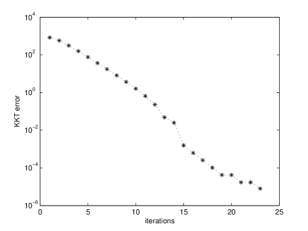
Fig. 1: KKT error versus iteration number for n = 200, m = 4, and ${\bf{A}}_{0}$ positive definite

The KKT error is computed using the formula given in Section 4 of [10]. Roughly, this formula amounts to the infinity norm of the gradient of the Lagrangian plus the infinity norm of the violation in complementary slackness. If ${\bf{A}}_{0}$ is constructed to have precisely one zero eigenvalue, then the convergence rate again appears to be linear, as seen in Figure 2.

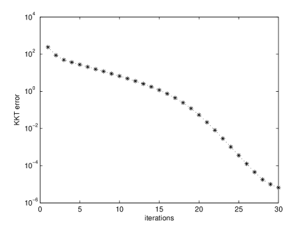
Fig. 2: KKT error versus iteration number for n = 200, m = 4, and a positive semidefinite ${\bf{A}}_{0}$.

7.2 Comparison with other algorithms for programs with convex cost

To gain some insight into the relative performance of the ball approximation algorithm (BAA), we solved randomly generated problems with convex cost using three other algorithms:

• SEDUMI, for optimization over symmetric cones.

• The gradient projection algorithm. We tried both the nonmonotone gradient project algorithm (NGPA) given in [11] and the nonmonotone spectral projected gradient method (SPG) of Birgin, Martínez, and Raydan [2, 3] (ACM Algorithm 813).

We now discuss in detail how each of these algorithms was implemented. The BAA subproblems (21) have the form

$$\min{\bf{x}}^{\sf T}{\bf{A}}_{0}{\bf{x}}+{\bf{b}}_{0}^{\sf T}{\bf{x}}\quad\mbox{ subject to }\|{\bf{x}}-{\bf{c}}_{i}\|^{2}\leq r_{i}^{2},\quad 1\leq i\leq m.$$ (36)

We solve these subproblems by applying the active set algorithm (ASA) developed in [11] to the dual problem. To facilitate the evaluation of the dual function, we compute the diagonalization ${\bf{A}}_{0}={\bf{QDQ}}^{\sf T}$ where ${\bf{D}}$ is diagonal and ${\bf{Q}}$ is orthogonal. Substituting ${\bf{x}}={\bf{Qy}}$ in (36) yields the equivalent problem

$$\min{\bf{y}}^{\sf T}{\bf{D}}{\bf{y}}+{\bf{b}}_{0}^{\sf T}{\bf{Qy}}\quad\mbox{ subject to }\|{\bf{y}}-{\bf{Q}}^{\sf T}{\bf{c}}_{i}\|^{2}\leq r_{i}^{2},\quad 1\leq i\leq m.$$

The dual problem is

$$\max_{\bm{\lambda}\geq{\bf{0}}}\;\;\min_{{\bf{y}}\in\mathbb{R}^{n}}\;\;{\bf{y}}^{\sf T}{\bf{Dy}}+{\bf{b}}_{0}^{\sf T}{\bf{Qy}}+\sum_{i=1}^{m}\lambda_{i}\left(\|{\bf{y}}-{\bf{Q}}^{\sf T}{\bf{c}}_{i}\|^{2}-r_{i}^{2}\right).$$ (37)

The $i$-th component of the gradient of the dual function with respect to $\bm{\lambda}$ is simply $\|{\bf{y}}(\bm{\lambda})-{\bf{Q}}^{\sf T}{\bf{c}}_{i}\|^{2}-r_{i}^{2}$ where ${\bf{y}}(\bm{\lambda})$ achieves the minimum in (37). This minimum is easily evaluated since the quadratic term in the objective function is diagonal.

SEDUMI could be applied directly to (QP) when the cost function is strongly convex. We used Version 1.1 of the code obtained from

http://sedumi.mcmaster.ca/

In implementing the gradient projection algorithm for (QP), we need to project a vector onto the feasible set. This amounts to solving a problem of the form

$$\min\|{\bf{x}}-{\bf{a}}\|^{2}\mbox{ subject to }{\bf{g}}({\bf{x}})\leq{\bf{0}}.$$

We solved this problem using BAA. An iteration of BAA reduces to the solution of a problem with the following structure:

$$\min\|{\bf{x}}-{\bf{a}}\|^{2}\mbox{ subject to }\|{\bf{x}}-{\bf{c}}_{i}\|^{2}\leq r_{i}^{2},\quad i=1,2,\ldots,m.$$ (38)

As in [16], we solve these problems by forming the dual problem

$$\max_{\bm{\lambda}\geq{\bf{0}}}\;\;\min_{{\bf{x}}\in\mathbb{R}^{n}}~{}\|{\bf{x}}-{\bf{a}}\|^{2}+\sum_{i=1}^{m}\lambda_{i}\left(\|{\bf{x}}-{\bf{c}}_{i}\|^{2}-r_{i}^{2}\right).$$

After carrying out the inner minimization, this reduces to

$$\max_{\bm{\lambda}\geq{\bf{0}}}-\frac{\|{\bf{a}}+\sum_{i=1}^{m}\lambda_{i}{\bf{c}}_{i}\|^{2}}{1+\sum_{i=1}^{m}\lambda_{i}}+\sum_{i=1}^{m}\lambda_{i}(\|{\bf{c}}_{i}\|^{2}-r_{i}^{2}).$$ (39)

If $\bm{\lambda}$ solves the dual problem (39), then the associated solution of the primal problem (38) is

$${\bf{x}}=\frac{{\bf{a}}+\sum_{i=1}^{m}\lambda_{i}{\bf{c}}_{i}}{1+\sum_{i=1}^{m}\lambda_{i}}.$$

Again, the dual problem (39) is solved using the active set algorithm (ASA) of [11].

The test problems used in Tables 1 and 2 were generated as follows:

Table 1: Positive definite cases

$n,m$		SED	success	BAA	success	NGPA	success	SPG	success
	time	0.52		0.07		4.70		5.94
100,4	iter	10.06	28	19.00	30	172.43	17	200.06	17
	time	2.75		0.32		10.68		11.76
200,4	iter	9.56	26	12.70	30	203.23	21	348.36	20
	time	8.14		0.72		128.19		122.23
300,4	iter	9.60	27	21.46	30	269.86	20	431.83	20
	time	20.13		1.64		404.28		438.84
400,4	iter	10.26	27	49.26	29	352.66	18	545.23	18
	time	44.07		2.54		579.21		647.56
500,4	iter	12.33	28	29.90	30	369.20	15	574.13	13
	time	57.28		4.27		648.79		611.60
600,4	iter	9.30	26	36.80	29	309.43	19	306.50	19
	time	3.51		0.08		86.89		81.67
100,40	iter	10.26	28	19.00	30	150.76	21	165.66	21
	time	26.56		0.32		268.63		250.22
200,40	iter	12.70	30	12.70	30	199.70	17	218.50	16
	time	54.56		0.81		732.50		727.92
200,100	iter	10.66	30	9.50	30	295.80	20	327.26	20
	time	23.84		0.72		579.62		530.02
100,200	iter	14.96	30	20.06	30	249.43	18	261.46	19
	time	0.093		0.002		3.02		2.75
4,100	iter	9.06	29	6.96	30	19.46	26	19.40	25
	time	0.114		0.004		6.23		5.70
4,200	iter	9.56	27	8.73	30	16.26	26	16.46	26
	time	0.148		0.012		13.45		11.58
4,300	iter	11.06	25	12.56	30	15.26	24	15.33	23
	time	0.195		0.014		16.27		12.87
4,400	iter	13.33	28	12.26	30	16.26	28	15.70	28
	time	0.221		0.017		21.08		18.16
4,500	iter	13.83	26	11.50	30	13.83	26	13.83	26
	time	0.235		0.018		31.65		34.83
4,600	iter	12.13	26	11.00	30	15.40	24	16.33	24

Let Rand$(n,l,u)$ denote a vector in $\mathbb{R}^{n}$ whose entries are chosen randomly in the interval $(l,u)$. Random positive definite matrices ${\bf{A}}$ are generated using the procedure given in [17], which we now summarize. Let ${\bf{w}}_{i}\in$ Rand$(n,-1,1)$ for $i=1$, 2, 3, and define

$${\bf{Q}}_{i}={\bf{I}}-2{\bf{v}}_{i}{\bf{v}}_{i}^{\sf T},\quad{\bf{v}}_{i}={\bf{w}}_{i}/\|{\bf{w}}_{i}\|.$$

Let ${\bf{D}}$ be a diagonal matrix with diagonal in Rand$(n,0,100)$. Finally, ${\bf{A}}={\bf{UDU}}^{\sf T}$ with ${\bf{U}}={\bf{Q}}_{1}{\bf{Q}}_{2}{\bf{Q}}_{3}$. To obtain a randomly generated positive semidefinite matrix, we use the same procedure, however, we randomly set one diagonal element of ${\bf{D}}$ to zero.

We make a special choice for $c_{i}$ to ensure that the feasible set for (QP) is nonempty. We first generate ${\bf{p}}\in$ Rand$(n,-50,50)$ and we set

$$c_{i}=-({\bf{p}}^{\sf T}{\bf{A}}_{i}{\bf{p}}+{\bf{b}}_{i}^{\sf T}{\bf{p}}+s_{i}),$$

where $s_{i}$ is randomly generated in the interval $[0,10]$ and ${\bf{b}}_{i}\in$ Rand$(n,-100,100)$. With this choice for $c_{i}$, the feasible set for (QP) is nonempty since ${\bf{p}}$ lies in the interior of the feasible set. The stopping criterion in our experiments was

$$\|P({\bf{x}}_{k}-{\bf{g}}_{k})-{\bf{x}}_{k}\|\leq 10^{-4},$$ (40)

where $P$ denotes projection into the feasible set for (QP) and ${\bf{g}}_{k}=2{\bf{A}}_{0}{\bf{x}}_{k}+{\bf{b}}_{0}$ is the gradient of the objective function at ${\bf{x}}_{k}$. When the cost is convex, the left side of (40) vanishes if and only if ${\bf{x}}_{k}$ is a solution of (QP).

Tables 1 and 2 report the average CPU time in seconds ($time$), the average number of iterations ($iter$), and the number of successes in 30 randomly generated test problems. The algorithm was considered successful if the error tolerance (40) was satisfied.

Table 2: Positive semidefinite cases

$n,m$		BAA	success	NGPA	success	SPG	success
	time	0.11		15.04		17.38
100,4	iter	42.16	30	328.53	22	408.20	19
	time	0.55		44.32		45.82
200,4	iter	99.33	30	313.10	20	356.43	22
	time	1.02		290.19		304.89
300,4	iter	74.23	30	374.13	22	417.60	21
	time	2.28		501.14		572.63
400,4	iter	111.83	30	404.66	19	492.83	19
	time	5.37		620.13		657.61
500,4	iter	200.03	27	382.66	16	478.60	17
	time	0.61		356.40		321.92
100,40	iter	82.30	30	276.56	22	237.23	21
	time	2.74		398.54		415.28
200,40	iter	127.23	30	369.43	17	416.060	17
	time	3.19		1030.02		949.29
100,200	iter	108.63	28	311.40	19	352.23	18
	time	0.054		16.74		14.25
4,100	iter	38.66	30	31.13	16	31.23	16
	time	0.075		44.74		33.24
4,200	iter	43.46	27	26.20	13	23.36	18
	time	0.076		111.03		100.38
4,300	iter	31.50	29	29.33	14	28.60	11
	time	0.049		205.17		237.62
4,400	iter	36.73	29	27.20	18	31.23	18
	time	0.065		229.77		247.82
4,500	iter	41.86	28	24.46	16	26.30	17

Based on our numerical experiments, it appears that BAA can achieve an error tolerance on the order of the square root of the machine epsilon [9, 24], similar to the computing precision which is achieved by interior point methods for linear programming prior to simplex crossover. The convergence tolerance (40) was chosen since it seems to approach the maximum accuracy which could be achieved by BAA in these test problems. Numerically, BAA seems to terminate when the solution to the subproblem (21) yields a direction which departs from the feasible set, and hence, the stepsize in the line search Step 2b is zero. We were able to achieve a further improvement in the solution by taking a partial step in this infeasible direction since the increase in constraint violation was much less than the improvement in objective function value. Nonetheless, the improvement in accuracy achieved by permitting infeasibility was at most one digit in our experiments.

In Tables 1 and 2 we see that BAA gave the best results for this test set, both in terms of CPU time and in terms of successes (the number of times that the convergence tolerance (40) was achieved). Recall that the gradient projection algorithms in our experiments used BAA to compute the projected gradient. The convergence failures for the gradient projection algorithms in Tables 1 and 2 were due to the fact that BAA was unable to compute the projected gradient with enough accuracy to yield descent in the gradient projection algorithm.

7.3 Problems with nonconvex cost

We tested our ellipsoidal branch and bound algorithm using some randomly generated test problems with ${\bf{A}}_{0}$ indefinite. To compute $\bm{\mu}$ in (7), we used the power method (see [24]) to find the eigenvector associated with the largest eigenvalue. We chose $\lambda$ in (2) to be 0.1 minus the smallest eigenvalue of ${\bf{A}}_{0}$. NGPA was used to locally solve (QP) and update the upper bound.

We took $m=2$ and randomly generated test problem using the procedure in [1]. That is, the ellipsoidal constraint functions in (QP) have the form

$$g_{i}({\bf{x}})=({\bf{x}}-{\bf{c}}_{i})^{\sf T}{\bf{B}}^{-1}_{i}({\bf{x}}-{\bf{c}}_{i})-1,$$

where ${\bf{B}}_{i}={\bf{UD}}_{i}{\bf{U}}^{\sf T}$ and ${\bf{U}}$ is as given earlier. ${\bf{D}}_{i}$ is a diagonal matrix with its diagonal in Rand$(n,0,60)$, ${\bf{c}}_{1}\in$ Rand$(n,0,100)$, and ${\bf{c}}_{2}={\bf{c}}_{1}+.8{\bf{v}}$ where ${\bf{v}}$ is the semi-major axis of the ellipsoid $g_{1}({\bf{x}})\leq 0$. For this choice of ${\bf{c}}_{2}$, the ellipsoids $g_{1}({\bf{x}})\leq 0$ and $g_{2}({\bf{x}})\leq 0$ have nonempty intersection at ${\bf{x}}={\bf{c}}_{2}$. In the objective function, ${\bf{A}}_{0}={\bf{U}}{\bf{D}}{\bf{U}}^{\sf T}$ where ${\bf{D}}$ is a diagonal matrix with diagonal in Rand$(n,-30,30)$ and ${\bf{b}}_{0}\in$ Rand$(n,-1,1)$. The case $m=2$ is especially important since quadratic problems with two ellipsoidal constraints belong to the class of Celis-Dennis-Tapia subproblems [4] which arise from the application of the trust region method for equality constrained nonlinear programming [12, 20, 6, 5, 15, 26, 19].

If $\mbox{UB}_{k}$ and $\mbox{LB}_{k}$ are the respective upper and lower bounds for the optimal objective function value at iteration $k$, then our stopping criterion was

$$\mbox{UB}_{k}-\mbox{LB}_{k}\leq\max\{\epsilon_{a},\epsilon_{r}|\mbox{LB}_{k}|\},$$

with $\epsilon_{a}=10^{-5}$ and $\epsilon_{r}=10^{-2}$.

We considered problems of 8 different dimensions ranging from 30 up to 300 as shown in Table 3. For each dimension, we solved 4 randomly generated problems. Table 3 shows the numerical results for our test instances, where “$neigs$” is the number of negative eigenvalues of the objective function, “$lb^{1}$” and “$ub^{1}$” are the lower bound and upper bounds at the first step, “val” is the computed optimal value and “it” is the number of iterations. We also report the performance of the algorithm for $m=6$ in Table 4.

Table 3: The performance of branch and bound algorithm for $m=2$

$n$	$neigs$	$lb^{1}$	$ub^{1}$	val	it	time
30	12	34827.3	35256.3	35254.8	5	1.75
	17	-41212.1	-40746.2	-40748.8	21	3.58
	14	38601.4	38977.6	38977.6	0	0.72
	17	-31534.2	-31108.4	-31119.8	92	8.82
50	22	-357168.8	-356828.8	-356828.8	0	0.52
	21	-33792.9	-33447.9	-33447.9	1	0.84
	21	-29694.6	-29254.1	-29255.2	247	23.08
	26	35034.0	35416.6	35414.8	5	2.12
60	29	17783.6	18227.4	18227.4	78	22.41
	26	-27498.2	-27110.5	-27110.5	69	18.22
	30	-69845.7	-69463.1	-69463.1	0	0.56
	28	20408.7	20963.1	20927.1	273	42.65
100	50	-11495.2	-11196.9	-11218.9	56	30.72
	51	17539.6	17909.3	17909.3	4	1.84
	52	-46065.5	-45653.2	-45653.2	0	0.88
	40	970829.8	971326.6	971326.6	0	0.92
150	75	-302382.2	-302071.0	-302071.0	0	0.95
	83	29089.4	29500.8	29500.8	64	31.45
	72	16580.5	16904.9	16904.9	1	1.98
	73	-32461.9	-32036.1	-32036.1	1	1.37
200	100	10798.5	11226.1	11226.1	81	56.58
	95	-27242.9	-26792.1	-26792.1	2	2.27
	100	35293.0	35862.1	35862.1	1	1.63
	96	-31712.8	-31138.3	-31138.3	77	47.06
250	135	37015.8	37477.6	37477.6	1	2.9
	131	-27278.9	-26563.0	-26780.0	86	88.40
	128	-9979.6	-9683.9	-9683.9	59	131.54
	121	-371385.9	-370991.9	-370991.9	0	2.03
300	145	-162041.5	-161645.7	-161645.7	0	5.33
	152	-48085.4	-47529.3	-47529.3	1	7.56
	138	226345.6	226377.8	226377.8	0	4.79
	148	-17649.5	-17013.7	-17323.2	109	257.52

In comparing our ellipsoidal branch and bound algorithm based on linear underestimation (EBL) to the ellipsoidal branch and bound algorithm of Le Thi Hoai An [1] based on dual underestimation (EBD), an advantage of EBD is that the underestimates are often quite tight in the dual-based approach. As seen in Table 3, EBL required up to 273 bisections for this test set while EBD in [1] was able to solve randomly generated test problems without any bisections. On the other hand, a disadvantage of EBD is that the dual problems are nondifferentiable when ${\bf{A}}_{0}$ is indefinite. Consequently, the evaluation of the lower bound using EBD entails solving an optimization problem which, in general, is nondifferentiable. With EBL, however, computing a lower bound involves solving a convex optimization problem. To summarize, EBD provides tight lower bounds using a nondifferentiable optimization problem for the lower bound, while EBL provides less tight lower bounds using a convex optimization problem for the lower bound.

Table 4: The performance of branch and bound algorithm for $m=6$

$n$	$neigs$	$lb^{1}$	$ub^{1}$	val	it	time
30	17	22717.1	22993.1	22993.1	1	2.41
	21	-22847.0	-22520.4	-22524.5	14	10.58
	20	-17858.2	-17573.2	-17573.2	1	1.84
60	33	-21818.1	-21489.1	-21489.2	33	21.64
	27	47683.8	47826.0	47826.0	0	2.82
	31	-4926.5	-4652.0	-4728.7	4	7.62
100	56	-35438.9	-35411.0	-35411.0	0	0.78
	52	-1740.1	-1187.5	-1198.2	354	283.25
	49	-6756.5	-6148.9	-6148.9	3	8.06

8 Conclusions

A globally convergent branch and bound algorithm was developed in which the objective function was written as the difference of convex functions. The algorithm was based on an affine underestimate given in Theorem 1 for the concave part of the objective function restricted to an ellipsoid. An algorithm of Lin and Han [16, 17] for projecting a point onto a convex set was generalized so as to replace their norm objective by an arbitrary convex function. This generalization could be employed in the branch and bound algorithm for a general objective function when the constraints are convex. Numerical experiments were given for a randomly generated quadratic objective function and randomly generated convex, quadratic constraints.

References

- [1] L. T. H. An, An efficient algorithm for globally minimizing a quadratic function under convex quadratic constraints, Math. Program., 87 (2000), pp. 401–426.
- [2] E. G. Birgin, J. M. Martínez, and M. Raydan, Nonmonotone spectral projected gradient methods for convex sets, SIAM J. Optim., 10 (2000), pp. 1196–1211.
- [3] , Algorithm 813: SPG - software for convex-constrained optimization, ACM Trans. Math. Softw., 27 (2001), pp. 340–349.
- [4] M. Celis, J. E. Dennis, and R. A. Tapia, A trust region strategy for nonlinear equality constrained optimization, in Numerical Optimization 1984, Philadelphia, PA, 1985, SIAM, pp. 71–82.
- [5] X. D. Chen and Y. Yuan, A note on quadratic forms, Math. Program., 86 (1999), pp. 187–197.
- [6] , On local solutions of the cdt subproblem, SIAM J. Optim., 10 (1999), pp. 359–383.
- [7] P. L. Combettes and T. Pennanen, Proximal methods for cohypomonotone otperators, SIAM J. Control, 43 (2004), pp. 731–742.
- [8] C. A. Floudas and V. Visweswaran, Quadratic optimization, in Handbook of Global Optimization, R.Horst and P. Pardalos, eds., Kluwer Academic, 1994, pp. 217–270.
- [9] W. W. Hager, Applied Numerical Linear Algebra, Prentice-Hall, Englewood Cliffs, NJ, 1988.
- [10] W. W. Hager and S. Gowda, Stability in the presence of degeneracy and error estimation, Math. Program., 85 (1999), pp. 181–192.
- [11] W. W. Hager and H. Zhang, A new active set algorithm for box constrained optimization, SIAM J. Optim., 17 (2006), pp. 526–557.
- [12] M. Heinkenschloss, On the solution of a two ball trust region subproblem, Math. Programming, 64 (1994), pp. 249–276.
- [13] R. Horst, P. M. Pardalos, and N. V. Thoai, Introduction to Global Optimization, Kluwer Academic Publishers, Dordrecht, Holland, 1995.
- [14] A. N. Iusem, T. Pennanen, and B. F. Svaiter, Inexact variants of the proximal point algorithm without monotonicity, SIAM J. Optim., 13 (2003), pp. 1080–1097.
- [15] G. D. Li and Y. Yuan, Computing a celis-dennis-tapia step, J. Comput. Math., 23 (2005), pp. 463–478.
- [16] A. Lin, A class of method for projection on a convex set, Advanced Modeling and Optimization, 5 (2003), pp. 211–221.
- [17] A. Lin and S. P. Han, A class of methods for projection on the intersection of several ellipsoids, SIAM J. Optim., 15 (2005), pp. 129–138.
- [18] J. Linderoth, A simplicial branch and bound algorithm for solving quadratically constrained quadratic programs, Math. Program., 103 (2005), pp. 251–282.
- [19] J. M. Martinez and S. A. Santos, A trust-region strategy for minimization on arbitrary domains, Math. Program., 68 (1995), pp. 267–301.
- [20] J. M. Peng and Y. Yuan, Optimality conditions for the minimization of a quadratic with two quadratic constraints, SIAM J. Optim., 7 (1997), pp. 579–594.
- [21] T. Pennanen, Local convergence of the proximal point algorithm and multiplier methods without monotonicity, Math. Oper. Res., 27 (2002), pp. 170–191.
- [22] U. Raber, A simplicial branch and bound method for solving nonconvex all-quadratic programs, J. Global Optim., 13 (1998), pp. 417–432.
- [23] N. Z. Shor, Cut-off method with space extension in convex programming problems, Cybernetics and System Analysis, 1 (1977), pp. 94–97.
- [24] L. N. Trefethen and D. Bau III, Numerical Linear Algebra, SIAM, Philadelphia, 1997.
- [25] J. P. Vial, Strong and weak convexity of sets and functions, Math. Oper. Res., 8(2) (1983), pp. 231–259.
- [26] Y. Ye and S. Zhang, New results on quadratic minimization, SIAM J. Optim., 14 (2003), pp. 245–267.
- [27] D. B. Yudin and A. S. Nemirovski, Informational complexity and effective methods for the solution of convex extremal problems, Ekonom. Mat. Metody., 12 (1976), pp. 550–559 (in Russian).