• psrchive and psrfits: Definition of the Stokes Parameters and Instrumental Basis Conventions

  W. van Straten^A,C, R. Manchester^B, S. Johnston^B, and J. Reynolds^{B
  A} Swinburne University of Technology, PO Box 218, Hawthorn VIC 3122, Australia
  ^B CSIRO Astronomy and Space Science, PO Box 76, Epping NSW 1710, Australia ^C Email: vanstraten.willem@gmail.com

  Abstract:

  This paper defines the mathematical convention adopted to describe an electromagnetic wave and its polarisation state, as implemented in the psrchive software and represented in the psrfits definition. Contrast is made between the convention that has been widely accepted by pulsar astronomers and the IAU/IEEE definitions of the Stokes parameters. The former is adopted as the PSR/IEEE convention, and a set of useful parameters are presented for describing the differences between the PSR/IEEE standard and the conventions (either implicit or explicit) that form part of the design of observatory instrumentation. To aid in the empirical determination of instrumental convention parameters, well-calibrated average polarisation profiles of PSR J0304+1932 and PSR J0742$-$2822 are presented at radio wavelengths of approximately 10, 20, and 40 cm.

  Keywords: methods:data analysis — polarisation — pulsars: general — techniques: polarimetric

1 Introduction

Since the early days of pulsar astronomy, observations of the polarisation properties of their radio signal have yielded a diverse range of information about these stars and their environment, including the properties of the pulsar emission mechanism (e.g. Taylor et al. 1971; Lyne & Manchester 1988; Edwards & Stappers 2004), the geometry of the pulsar magnetosphere (e.g. Radhakrishnan & Cooke 1969; Johnston et al. 2005), and the properties of the Galactic magnetic field (e.g. Manchester 1974; Han et al. 2006). Polarimetry also provides additional information that may be exploited for high-precision pulsar timing (van Straten 2006).

Pulsars are typically observed either at the focus of a single antenna or at the phase centre of an antenna array. In either case, there are effectively two receptors that ideally respond maximally to orthogonal senses of polarisation. The statistical properties of the voltages induced in the receptors are computed as a function of topocentric pulse phase, producing a quantity known as the polarisation profile. Well-calibrated polarisation profiles require observations of one or more calibrator signals and a mathematical description of the instrumental response (e.g. van Straten 2004).

Even after calibration, there is often confusion regarding the definition of left-handed and right-handed circular polarisation (LCP and RCP) as well as the sign of Stokes $V$ and/or the position angle of the linear polarisation. The uncertainty arises from the different conventions that have persisted in the classical physics and engineering literature. The earliest pulsar polarisation observations (e.g. Manchester 1971) established a convention that is consistent with the Institute of Electrical and Electronics Engineers (IEEE) definition of LCP and RCP and the definition of Stokes $V$ by Kraus (1966). This convention differs from the one later adopted by the International Astronomical Union (IAU 1974).

The PSR/IEEE convention is implemented by the psrchive software and encoded in the psrfits file format, both of which have been openly developed in an effort to facilitate the exchange of pulsar astronomical data between observatories and research groups (Hotan et al. 2004). The psrchive software implements innovative methods of polarisation calibration (e.g. van Straten 2004, 2006) and Faraday rotation measure estimation (e.g. Han et al. 2006; Noutsos et al. 2008). To properly utilise these algorithms, data must be input in a form that complies with the PSR/IEEE convention.

In the following section, the PSR/IEEE convention is defined and contrasted with the IAU/IEEE definitions of the Stokes parameters. Section 3 introduces a comprehensive set of parameters that can be used to document the differences between an instrumental design and the PSR/IEEE convention. In Section 4, polarisation profiles of PSR J0304+1932 (B0301+19) and PSR J0742$-$2822 (B0740$-$28) are provided as a point of reference for astronomers aiming to conform to the PSR/IEEE convention.

2 Definitions

Consider a quasi-monochromatic electromagnetic wave with mean frequency $\omega$, represented at the origin by the transverse electric field vector

$$\mbox{\boldmath$e$}(t)=\left(\begin{array}[]{c}e_{0}\\ e_{1}\end{array}\right)=\left(\begin{array}[]{c}a_{0}(t)\exp i[\phi_{0}(t)+\omega t]\\ a_{1}(t)\exp i[\phi_{1}(t)+\omega t]\end{array}\right).$$ (1)

Note that the complex argument increases linearly with time; this sign convention is commonly encountered in engineering texts (e.g. Papoulis 1962; Bracewell 1965; Kraus 1966) and is implicit in the definition of most forward discrete Fourier transform (DFT) implementations (e.g. Frigo & Johnson 2005). It is also adopted in a seminal series of papers on radio polarimetric calibration (Hamaker et al. 1996; Sault et al. 1996; Hamaker & Bregman 1996). Given the above definition, time delays correspond to negative values of the phase $\phi$.

The polarisation of an electromagnetic wave is described by the second-order statistics of $e$, as represented using the complex $2\times 2$ coherency matrix (Born & Wolf 1980)

$$\mbox{\boldmath$\rho$}=\langle\mbox{\boldmath$e$}\,\mbox{\boldmath$\otimes\,e$}^{\dagger}\rangle=\left(\begin{array}[]{cc}\langle e_{0}e_{0}^{*}\rangle&\langle e_{0}e_{1}^{*}\rangle\\ \langle e_{1}e_{0}^{*}\rangle&\langle e_{1}e_{1}^{*}\rangle\end{array}\right).$$ (2)

Here, the angular brackets denote an ensemble average, $\otimes$ is the matrix direct product, and $\mbox{\boldmath$e$}^{\dagger}$ is the Hermitian transpose of $e$. The coherency matrix may be expressed as a linear combination of Hermitian basis matrices,

$${\mbox{\boldmath$\rho$}}={1\over 2}\sum_{k=0}^{3}S_{k}{\mbox{\boldmath$\sigma$}}_{k}=(S_{0}\,{\mbox{\boldmath$\sigma$}}_{0}+\mbox{\boldmath$S\cdot\sigma$})/2,$$ (3)

where $S_{0}$ is the total intensity, $\mbox{\boldmath$S$}=(S_{1},S_{2},S_{3})$ is the Stokes polarisation vector, ${\mbox{\boldmath$\sigma$}}_{0}$ is the $2\times 2$ identity matrix, and $\mbox{\boldmath$\sigma$}=({\mbox{\boldmath$\sigma$}}_{1},{\mbox{\boldmath$\sigma$}}_{2},{\mbox{\boldmath$\sigma$}}_{3})$ is a three-vector with components equal to the Pauli matrices. The four Hermitian basis matrices, consisting of the identity matrix and the three Pauli matrices, are defined as

$${\mbox{\boldmath$\sigma$}}_{0}=\left(\begin{array}[]{cc}1&0\\ 0&1\end{array}\right) {\mbox{\boldmath$\sigma$}}_{1}=\left(\begin{array}[]{cc}1&0\\ 0&-1\end{array}\right)$$ (8)

$${\mbox{\boldmath$\sigma$}}_{2}=\left(\begin{array}[]{cc}0&1\\ 1&0\end{array}\right) {\mbox{\boldmath$\sigma$}}_{3}=\left(\begin{array}[]{cc}0&-i\\ i&0\end{array}\right).$$ (13)

The Stokes parameters are the projections of the coherency matrix onto the basis matrices, given by

$$S_{k}={\rm tr}({\mbox{\boldmath$\sigma$}}_{k}\mbox{\boldmath$\rho$}),$$ (14)

where ${\rm tr}()$ is the matrix trace operator.

Linear transformations of the electric field are represented by complex $2\times 2$ Jones matrices. Under the operation, $\mbox{\boldmath$e$}^{\prime}=\textbf{{J}}\mbox{\boldmath$e$}$, the coherency matrix is subjected to a congruence transformation, ${\mbox{\boldmath$\rho$}^{\prime}}=\textbf{{J}}\mbox{\boldmath$\rho$}\textbf{{J}}^{\dagger}$. Using the axis-angle parameterisation (Britton 2000), the polar decomposition of a Jones matrix (Hamaker 2000) is expressed as

$$\textbf{{J}}=J\,{\textbf{{B}}}_{\mbox{\scriptsize\boldmath$\hat{m}$}}(\beta)\,{\textbf{{R}}}_{\mbox{\scriptsize\boldmath$\hat{n}$}}(\phi),$$ (15)

where $J=|\textbf{{J}}|^{1/2}$, $|\textbf{{J}}|$ is the determinant of J, ${\textbf{{B}}}_{\mbox{\scriptsize\boldmath$\hat{m}$}}(\beta)$ is positive-definite Hermitian, and ${\textbf{{R}}}_{\mbox{\scriptsize\boldmath$\hat{n}$}}(\phi)$ is unitary; both ${\textbf{{B}}}_{\mbox{\scriptsize\boldmath$\hat{m}$}}(\beta)$ and ${\textbf{{R}}}_{\mbox{\scriptsize\boldmath$\hat{n}$}}(\phi)$ are unimodular. Under the congruence transformation of the coherency matrix, the Hermitian matrix

$${\textbf{{B}}}_{\mbox{\scriptsize\boldmath$\hat{m}$}}(\beta)={\mbox{\boldmath$\sigma$}}_{0}\cosh\beta+\mbox{\boldmath$\hat{m}\cdot\sigma$}\sinh\beta$$ (16)

effects a Lorentz boost of the Stokes four-vector along the $\hat{m}$ axis by a hyperbolic angle $2\beta$. As the Lorentz transformation of a spacetime event mixes temporal and spatial dimensions, the polarimetric boost mixes total and polarised intensities, thereby altering the degree of polarisation. In contrast, the unitary matrix

$${\textbf{{R}}}_{\mbox{\scriptsize\boldmath$\hat{n}$}}(\phi)={\mbox{\boldmath$\sigma$}}_{0}\cos\phi+i\mbox{\boldmath$\hat{n}\cdot\sigma$}\sin\phi$$ (17)

rotates the Stokes polarisation vector about the $\hat{n}$ axis by an angle $2\phi$. As the orthogonal transformation of a vector in Euclidean space preserves its length, the polarimetric rotation leaves the total intensity and degree of polarisation unchanged.

2.1 The IAU/IEEE Convention

As summarised by Hamaker & Bregman (1996) and depicted in Figure 1, the IAU/IEEE definitions of the Stokes parameters are based on a right-handed Cartesian coordinate system, in which the plane wave propagates toward the observer in the positive $z$ direction, and $e_{0}=e_{x}$ and $e_{1}=e_{y}$ are the components of the electric field projected onto North and East, respectively. Noting that the sign of the complex argument in equation (1) corresponds to the upper sign convention in equations (2) through (4) of Hamaker & Bregman (1996), the Stokes parameters are defined by

$$I = \langle|e_{x}|^{2}+|e_{y}|^{2}\rangle$$ (18)

$$Q = \langle|e_{x}|^{2}-|e_{y}|^{2}\rangle$$ (19)

$$U = \langle 2\rm Re[e_{x}e_{y}^{*}]\rangle$$ (20)

$$V = \langle 2\rm Im[e_{x}e_{y}^{*}]\rangle$$ (21)

Stokes $V$ is positive for RCP, for which $e_{y}$ lags $e_{x}$ and, looking toward the source, the observer sees the electric field rotate counter-clockwise. The position angle of the linearly polarised component is also measured in a counter-clockwise direction from North toward East.

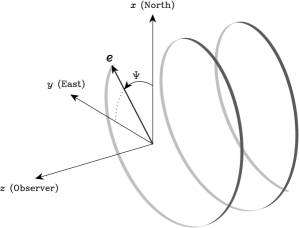
Figure 1: A right-hand circularly polarised (RCP) wave in the adopted coordinate system. The $x$ and $y$ axes lie in the plane of the sky, with the $x$-axis pointing North, the $y$-axis pointing East, and the $z$-axis pointing toward the observer. The electric field vector $e$ lies in the $x$–$y$ plane; its position angle $\Psi$ is measured with respect to North, increasing toward East. As the RCP wave propagates in the positive $z$ direction, the position angle increases; that is, the electric field vector rotates counter-clockwise, as seen by the observer. Note that an RCP wave, as defined by the IEEE, forms a left-handed helix in space.

2.2 The PSR/IEEE Convention

In the majority of published pulsar polarisation observations, Stokes $V$ is positive for LCP as defined by the IEEE (e.g. Manchester 1971; Stinebring et al. 1984; Xilouris et al. 1998). This is the convention described by Kraus (1966); it is encoded in the sign of the phase in equation (1), the definition of the Pauli matrices in equation (13), and the relationships between the Stokes parameters and the coherency matrix defined by equations (3) and (14). Using either equation (2) or equation (3) with $\mbox{\boldmath$S$}=(Q,U,V)$, it can be shown that in the linear basis,

$$\mbox{\boldmath$\rho$}={1\over 2}\left(\begin{array}[]{cc}I+Q&U-iV\\ U+iV&I-Q\end{array}\right).$$ (22)

In this case,

$$U+iV=2\langle e_{y}e_{x}^{*}\rangle.$$ (23)

That is, Stokes $V$ is positive when the phase of $e_{y}$ leads that of $e_{x}$, which is opposite to the IAU convention for Stokes $V$. The PSR/IEEE convention is adopted and used in the remainder of this paper; it is the standard implemented by the psrchive software and expressed in the psrfits definition.

The PSR/IEEE convention for the position angle of the linear polarisation is consistent with the IAU/IEEE convention. However, as discussed in detail by Everett & Weisberg (2001), the rotating vector model (RVM; Radhakrishnan & Cooke 1969) has often been applied to measurements using an equation in which the position angle is assumed to increase in a clockwise direction on the sky, which is opposite to the IAU/IEEE convention. Therefore, care must be taken when comparing RVM parameter estimates from different experiments.

Given the definition of the Stokes parameters in terms of linearly polarised receptors, it is possible to also define a standard basis for circularly polarised feeds. The basis transformation, C, is chosen to effect a convenient cyclic permutation of the Stokes parameters; that is, under the congruence transformation, $\mbox{\boldmath$\rho$}^{\prime}=\textbf{{C}}\mbox{\boldmath$\rho$}\textbf{{C}}^{\dagger}$, the Stokes vector, $\mbox{\boldmath$S$}^{\prime}=(V,Q,U)$.

The transformation with unit determinant that effects the desired cyclic permutation of the Stokes parameters is

$$\textbf{{C}}={1\over\sqrt{2i}}\left(\begin{array}[]{cc}1&-i\\ 1&i\end{array}\right)=(\mbox{\boldmath$e$}_{L}\;\mbox{\boldmath$e$}_{R})^{\dagger},$$ (24)

where

$$\mbox{\boldmath$e$}_{L}={1\over\sqrt{2i}}\left(\begin{array}[]{c}1\\ i\end{array}\right) \mathrm{and} \mbox{\boldmath$e$}_{R}={1\over\sqrt{2i}}\left(\begin{array}[]{c}1\\ -i\end{array}\right)$$ (29)

are the Jones vectors of left and right circularly polarised receptors expressed in the linear basis. Apart from an absolute phase factor of $e^{-i\pi/4}$ chosen to yield a basis transformation with unit determinant, the above definition of circularly polarised receptors is identical to that of Hamaker & Bregman (1996).

3 Instrumental Conventions

A wide variety of different conventions, both explicit definitions and implicit assumptions, are encountered in the design of observatory instrumentation and data analysis software. Therefore, it is desirable to define a set of parameters that describe any known differences between the experimental design and the chosen standard. These corrections can be be broadly classified into four groups: projection, basis, instrument, and backend.

The known projection of the ideal feed receptors onto the plane of the sky may include effects such as the parallactic rotation of an altitude-azimuth mounted antenna, or the foreshortening of fixed dipoles in an array. The ideal basis describes a feed consisting of two orthogonally polarised receptors with unit gain. The feed may also be equipped with an internal reference source, such as a noise diode, that may be used to calibrate the differential gain and phase of the instrumentation. The instrument parameterises the transformation from the receptors to the backend, as determined using a separate calibration procedure (e.g. van Straten 2004). The backend includes all hardware and software involved in reducing the astronomical data to produce results that are suitable for further analysis. Only the basis and backend correction parameterisations are discussed here.

3.1 Basis Parameters

In principle, the polarisations of both an ideal feed and the reference source could be specified by four rotations; e.g. two sets of ellipticity and orientation angles (Chandrasekhar 1960). However, basis rotations can be problematic due to singularities at the poles. Furthermore, it may be preferable to use less abstract, more commonly encountered, and/or more readily measured quantities. The convention may also be simplified by assuming that the receptors are either linearly or circularly polarised, and that the reference source is linearly polarised. Under these assumptions, the following four parameters are sufficient to completely describe the receiver.

Feed Basis: circularly or linearly polarised receptors

Feed Hand: left or right; if left, $e_{0}$ and $e_{1}$ are switched

Symmetry Angle: orientation of a linearly polarised signal that produces an equal and in-phase response in each receptor

Calibrator Phase: differential phase of the internal reference source, $\Phi_{c}=\tan^{-1}(S_{3}/S_{2})$

In the linear basis, a linearly polarised wave oscillating in the Northeast-to-Southwest plane (positive Stokes $U$) will produce equal and in-phase responses in each receptor; therefore, the symmetry angle has a nominal value of 45 degrees. Also, because the reference source is linearly polarised ($S_{3}=V=0$), there are only two possible values for the calibrator phase: 0 ($U>0$) and 180 ($U<0$) degrees.

In the circular basis, a linearly polarised wave oscillating in the North-to-South plane (positive Stokes $Q$) will produce equal and in-phase responses in each receptor; therefore, the symmetry angle has a nominal value of 0 degrees. Also, because $S_{2}=Q$ and $S_{3}=U$, the calibrator phase is arbitrary.

Given these parameters, the Jones matrix of the feed is given by

$$\textbf{{J}}=\textbf{{X}}\textbf{{C}}{\textbf{{R}}}_{\mbox{\scriptsize\boldmath$\hat{v}$}}(\Theta),$$ (30)

where X is the identity in a right-handed system and the exchange matrix in a left-handed system, C is the identity in the linear basis and given by equation (24) in the circular basis, and $\Theta$ is equal to the symmetry angle less its nominal value (45 degrees in the linear basis and 0 degrees in the circular basis). Note that, as defined by equation (17), ${\textbf{{R}}}_{\mbox{\scriptsize\boldmath$\hat{v}$}}(\Theta)$ effects a rotation of the Stokes polarisation vector about the Stokes $V$ axis by an angle $2\Theta$. The coherency matrix of the internal reference source is

$$\mbox{\boldmath$\rho_{c}$}={1\over 2}\left(\begin{array}[]{cc}1&\exp(-i\Phi_{c})\\ \exp(i\Phi_{c})&1\end{array}\right),$$ (31)

where $\Phi_{c}$ is the calibrator phase.

3.2 Backend parameters

To describe the design of the backend, it is sufficient to consider only the complex conjugation of the electric field. This occurs during lower sideband down conversion and/or when the design of an instrument is based upon a different convention for the sign of the phase than that adopted in equation (1). In the case of dual-sideband down conversion, complex conjugation occurs when the phase of the quadrature component leads that of the in-phase component of the signal. Complex conjugation causes a sign change in $S_{3}$, a reflection that cannot be represented by a Jones matrix. The following two parameters are used to describe the backend.

Backend Phase: positive or negative

Down Conversion: true or false; if true, the conjugation due to lower sideband down conversion has been corrected

The correction of complex conjugation is performed when either of the following conditions is exclusively true:

1. backend phase is negative, or

2. down conversion is false and lower sideband down conversion was used.

The correction is not performed when both A and B are true because they negate each other.

3.3 Implementation

Each of the parameters described in the preceding sections has a corresponding parameter in the psrfits definition and a representation in the psrchive software. Table 1 summarises these parameters, the range of acceptable values for each parameter, and the effects that they have on calibrated data.

Table 1: Instrumental convention parameters and their effects in each basis.

Parameter	psrfits	Range	Effect
	Name		Linear	Circular
Backend Phase	BE_PHASE	$\pm$1	$\pm$ V	$\pm$ U
Down conversiona	BE_DCC	0/1	$\pm$ V	$\pm$ U
Feed Basis	FD_POLN	LIN or CIRC	(Q,U,V)	(V,Q,U)
Feed Hand	FD_HAND	$\pm$ 1	$\pm$ Q&V	$\pm$ U&V
Symmetry Angle	FD_SANG	$-\pi/2<\theta<\pi/2$	${\textbf{{R}}}_{\mbox{\scriptsize\boldmath$\hat{v}$}}(\theta-\pi/4)$	${\textbf{{R}}}_{\mbox{\scriptsize\boldmath$\hat{v}$}}(\theta)$
Calibrator Phaseb	FD_XYPH	$-\pi<\Phi_{c}<\pi$	$\pm$ U&V	${\textbf{{R}}}_{\mbox{\scriptsize\boldmath$\hat{v}$}}(\Phi_{c}/2)$

^a Applies only when down conversion is effectively lower sideband.

^b In the linear basis, $\Phi_{c}=0$ or $\pi$.

4 Discussion

In general, it is non-trivial to determine the instrumental convention parameters from first principles and an empirical approach must be adopted. This typically requires observations of either artificial sources with known polarisation or astronomical sources that have been previously well calibrated, such as the average polarisation profiles of PSR J0304+1932 and PSR J0742$-$2822 presented in Figure 2. These sources are visible to observatories in both Northern and Southern hemispheres; they also have relatively high flux densities, well-defined position angle variation, and sufficient circular polarisation for the purposes of comparison with other observations.

These data were recorded at the Parkes Observatory on 2009 October 9 and 10 using the 64 m antenna and two of the Parkes Digital Filter Banks (PDFB3 and PDFB4). For each pulsar, a 256 MHz band centred at 1369 MHz was observed using the centre beam of the 20 cm Multibeam receiver and two bands, one with 64 MHz of bandwidth centred at 732 MHz and one with 1024 MHz of bandwidth centred at 3.1 GHz, were observed using the 10-50 cm dual-band receiver. Prior to each pulsar observation, a noise diode coupled to the receptors was observed and used to calibrate the differential gain and phase of the instrument. For the 20 cm observations, the receptor cross-coupling parameters were calibrated as described in van Straten (2004). Absolute flux calibration was performed using observations of the noise diode recorded while pointing on and off the bright Fanaroff-Riley type I radio galaxy, 3C 218 (Hydra A), which was assumed to have a flux density of 43.1 Jy at 1400 MHz and a spectral index of 0.91.

Figure 2: Average polarisation profiles of PSR J0304+1932 (left) and PSR J0742$-$2822 (right), observed at radio wavelengths of approximately 40 cm (top), 20 cm (middle), and 10 cm (bottom). In each plot, the lower panel displays the total intensity, Stokes $I$ (solid); the linearly polarised flux, $L=\sqrt{Q^{2}+U^{2}}$ (dashed); and the circular polarisation, Stokes $V$ (dotted); the upper panel plots the position angle of the linear polarisation, $\Psi=0.5\tan^{-1}(U/Q)$ (the error bars are two standard deviations in length). Stokes $V$ is positive for left-hand circularly polarised radiation as defined by the IEEE.

The data were corrected for Faraday rotation using the most recently published rotation measure (RM) for each pulsar, as determined using the ATNF Pulsar Catalogue (Manchester et al. 2005). For PSR J0304+1932, RM=$-8.3$ rad m^-2 (Manchester 1974); for PSR J0742$-$2822, RM=+149.95 rad m^-2 (Johnston et al. 2005). The position angles plotted in Figure 2 are referred to the centre frequency of the band and are as observed at Parkes. Variations in the Faraday rotation along the line of sight, particularly those occurring in the Earth’s ionosphere, will rotate the observed angles by a small amount. The ionospheric RM component was estimated using the International Reference Ionosphere models (Bilitza 2001) and was about $-0.7$ rad m^-2 in the direction of PSR J0304+1932 and $-1.5$ rad m^-2 in the direction of PSR J0742$-$2822. Position angles above the ionosphere were therefore greater than the plotted values by about $0\mbox{$.\!\!^{\circ}$}4$ and $0\mbox{$.\!\!^{\circ}$}8$ at 3100 MHz, $0\mbox{$.\!\!^{\circ}$}7$ and $1\mbox{$.\!\!^{\circ}$}5$ at 1369 MHz, and $7\mbox{$.\!\!^{\circ}$}5$ and $14\mbox{$.\!\!^{\circ}$}4$ at 732 MHz for PSR J0304+1932 and PSR J0742$-$2822 respectively.

Referring to the effects defined in Table 1, the instrumental convention parameters of new systems can be adjusted until the observed values of Stokes $V$ and position angle match those plotted in Figure 2. This comparison should be performed only after the projection (e.g. parallactic rotation) and instrument (e.g. differential gain and phase) have been calibrated. Given the overlapping domains of the parameter effects, the proper selection of parameter values will most likely require consultation with both engineering documentation and observatory staff.

References

- Bilitza (2001) Bilitza, D. 2001, Radio Sci., 36, 261
- Born & Wolf (1980) Born, M. & Wolf, E. 1980, Principles of optics: electromagnetic theory of propagation ,interference and diffraction of light (New York: Pergamon)
- Bracewell (1965) Bracewell, R. 1965, The Fourier Transform and its Applications (New York: McGraw–Hill)
- Britton (2000) Britton, M. C. 2000, ApJ, 532, 1240
- Chandrasekhar (1960) Chandrasekhar, S. 1960, Radiative transfer (New York: Dover, 1960)
- Edwards & Stappers (2004) Edwards, R. T. & Stappers, B. W. 2004, A&A, 421, 681
- Everett & Weisberg (2001) Everett, J. E. & Weisberg, J. M. 2001, ApJ, 553, 341
- Frigo & Johnson (2005) Frigo, M. & Johnson, S. G. 2005, Proceedings of the IEEE, 93, 216
- Hamaker (2000) Hamaker, J. P. 2000, A&AS, 143, 515
- Hamaker & Bregman (1996) Hamaker, J. P. & Bregman, J. D. 1996, A&AS, 117, 161
- Hamaker et al. (1996) Hamaker, J. P., Bregman, J. D., & Sault, R. J. 1996, A&AS, 117, 137
- Han et al. (2006) Han, J. L., Manchester, R. N., Lyne, A. G., Qiao, G. J., & van Straten, W. 2006, ApJ, 642, 868
- Hotan et al. (2004) Hotan, A. W., van Straten, W., & Manchester, R. N. 2004, PASA, 21, 302
- IAU (1974) IAU. 1974, Transactions of the IAU, 15B, 166
- Johnston et al. (2005) Johnston, S., Hobbs, G., Vigeland, S., Kramer, M., Weisberg, J. M., & Lyne, A. G. 2005, MNRAS, 364, 1397
- Kraus (1966) Kraus, J. D. 1966, Radio astronomy (New York: McGraw-Hill)
- Lyne & Manchester (1988) Lyne, A. G. & Manchester, R. N. 1988, MNRAS, 234, 477
- Manchester (1971) Manchester, R. N. 1971, ApJS, 23, 283
- Manchester (1974) —. 1974, ApJ, 188, 637
- Manchester et al. (2005) Manchester, R. N., Hobbs, G. B., Teoh, A., & Hobbs, M. 2005, AJ, 129, 1993
- Noutsos et al. (2008) Noutsos, A., Johnston, S., Kramer, M., & Karastergiou, A. 2008, MNRAS, 386, 1881
- Papoulis (1962) Papoulis, A. 1962, The Fourier Integral and Its Applications (London: McGraw-Hill)
- Radhakrishnan & Cooke (1969) Radhakrishnan, V. & Cooke, D. J. 1969, Astrophys. Lett., 3, 225
- Sault et al. (1996) Sault, R. J., Hamaker, J. P., & Bregman, J. D. 1996, A&AS, 117, 149
- Stinebring et al. (1984) Stinebring, D. R., Cordes, J. M., Rankin, J. M., Weisberg, J. M., & Boriakoff, V. 1984, ApJS, 55, 247
- Taylor et al. (1971) Taylor, J. H., Huguenin, G. R., Hirsch, R. M., & Manchester, R. N. 1971, Astrophys. Lett., 9, 205
- van Straten (2004) van Straten, W. 2004, ApJ, 152, 129
- van Straten (2006) —. 2006, ApJ, 642, 1004
- Xilouris et al. (1998) Xilouris, K. M., Kramer, M., Jessner, A., von Hoensbroech, A., Lorimer, D., Wielebinski, R., Wolszczan, A., & Camilo, F. 1998, ApJ, 501, 286