Gradient-based methods for sparse recovery

Abstract

The convergence rate is analyzed for the SpaSRA algorithm (Sparse Reconstruction by Separable Approximation) for minimizing a sum $f({\bf{x}})+\psi({\bf{x}})$ where $f$ is smooth and $\psi$ is convex, but possibly nonsmooth. It is shown that if $f$ is convex, then the error in the objective function at iteration $k$, for $k$ sufficiently large, is bounded by $a/(b+k)$ for suitable choices of $a$ and $b$. Moreover, if the objective function is strongly convex, then the convergence is $R$-linear. An improved version of the algorithm based on a cycle version of the BB iteration and an adaptive line search is given. The performance of the algorithm is investigated using applications in the areas of signal processing and image reconstruction.

1 Introduction

In this paper we consider the following optimization problem

$$\min_{{\bf{x}}\in\mathbb{R}^{n}}\;\;\phi({\bf{x}}):=f({\bf{x}})+\psi({\bf{x}}),$$ (1)

where $f:\mathbb{R}^{n}\rightarrow\mathbb{R}$ is a smooth function, and $\psi:\mathbb{R}^{n}\rightarrow\mathbb{R}$ is convex. The function $\psi$, usually called the regularizer or regularization function, is finite for all ${\bf{x}}\in\mathbb{R}^{n}$, but possibly nonsmooth. An important application of (1), found in the signal processing literature, is the well-known $\ell_{2}-\ell_{1}$ problem (called basis pursuit denoising in [7])

$$\min_{{\bf{x}}\in\mathbb{R}^{n}}\;\;\frac{1}{2}\|{\bf{A}}{\bf{x}}-{\bf{b}}\|^{2}_{2}+\tau\|{\bf{x}}\|_{1},$$ (2)

where ${\bf{A}}\in\mathbb{R}^{k\times n}$ (usually $k\leq n$), ${\bf{b}}\in\mathbb{R}^{k},\tau\in\mathbb{R}$, $\tau\geq 0$, and $\|\cdot\|_{1}$ is the $1$-norm.

Recently, Wright, Nowak, and Figueiredo [24] introduced the Sparse Reconstruction by Separable Approximation algorithm (SpaRSA) for solving (1). The algorithm has been shown to work well in practice. In [24] the authors establish global convergence of SpaRSA. In this paper, we prove an estimate of the form $a/(b+k)$ for the error in the objective function when $f$ is convex. If the objective function is strongly convex, then the convergence of the objective function and the iterates is at least R-linear. A strategy is presented for improving the performance of SpaRSA based on a cyclic Barzilai-Borwein step [8, 9, 13, 19] and an adaptive choice [15] for the reference function value in the line search. The paper concludes with a series of numerical experiments in the areas of signal processing and image reconstruction.

Throughout the paper $\nabla f({\bf{x}})$ denotes the gradient of $f$, a row vector. The gradient of $f({\bf{x}})$, arranged as a column vector, is ${\bf{g}}({\bf{x}})$. The subscript $k$ often represents the iteration number in an algorithm, and ${\bf{g}}_{k}$ stands for ${\bf{g}}({\bf{x}}_{k})$. $\|\cdot\|$ denotes $\|\cdot\|_{2}$, the Euclidean norm. $\partial\psi({\bf{y}})$ is the subdifferential at ${\bf{y}}$, a set of row vectors. If ${\bf{p}}\in\partial\psi({\bf{y}})$, then

$$\psi({\bf{x}})\geq\psi({\bf{y}})+{\bf{p}}({\bf{x}}-{\bf{y}})$$

for all ${\bf{x}}\in\mathbb{R}^{n}$.

2 The SpaRSA algorithm

The SpaRSA algorithm, as presented in [24], is as follows:

Sparse Reconstruction by Separable Approximation (SpaRSA)
Given $\eta>1$, $\sigma\in(0,1)$, $[\alpha_{\min},\alpha_{\max}]\subset(0,\infty)$, and starting guess ${\bf{x}}_{1}$.
Set $k=1$.
Step 1. Choose $\alpha_{0}\in[\alpha_{\min},\alpha_{\max}]$ Step 2. Set $\alpha=\eta^{j}\alpha_{0}$ where $j\geq 0$ is the smallest integer such that $\phi({\bf{x}}_{k+1})\leq\phi_{k}^{R}-\sigma\alpha\|{\bf{x}}_{k+1}-{\bf{x}}_{k}\|^{2}$ where ${\bf{x}}_{k+1}=\mbox{arg}\min\{\nabla f({\bf{x}}_{k}){\bf{z}}+\alpha\|{\bf{z}}-{\bf{x}}_{k}\|^{2}+\psi({\bf{z}}):{\bf{z}}\in\mathbb{R}^{n}\}$. Step 3. If ${\bf{x}}_{k+1}={\bf{x}}_{k}$, terminate. Step 4. Set $k=k+1$ and go to step 1.

The parameter $\alpha_{0}$ in [24] was taken to be the BB parameter [1] with safeguards:

$$\alpha_{0}=\alpha^{BB}_{k}=\min\;\;\{\|\alpha{\bf{s}}_{k}-{\bf{y}}_{k}\|:\alpha_{\min}\leq\alpha\leq\alpha_{\max}\}$$ (3)

where ${\bf{s}}_{k}={\bf{x}}_{k}-{\bf{x}}_{k-1}$ and ${\bf{y}}_{k}={\bf{g}}_{k}-{\bf{g}}_{k-1}$. Also, in [24], the reference value $\phi_{k}^{R}$ is the GLL [14] reference value $\phi_{k}^{\max}$ defined by

$$\phi_{k}^{\max}=\max\{\phi({\bf{x}}_{k-j}):0\leq j<\min(k,M)\}.$$ (4)

In other words, at iteration $k$, $\phi_{k}^{\max}$ is the maximum of the $M$ most recent values for the objective function. Note that if ${\bf{x}}_{k+1}={\bf{x}}_{k}$, then

$${\bf{0}}\in\nabla f({\bf{x}}_{k})+\partial\psi({\bf{x}}_{k+1})=\nabla f({\bf{x}}_{k+1})+\partial\psi({\bf{x}}_{k+1}).$$

Hence, ${\bf{x}}_{k+1}={\bf{x}}_{k}$ is a stationary point.

The overall structure of the SpaRSA algorithm is closely related to that of the Iterative Shrinkage Thresholding Algorithm (ISTA) [6, 10, 12, 16, 23]. ISTA, however, employs a fixed choice for $\alpha$ related to the Lipschitz constant for $f$, while SpaRSA employs a nonmonotone line search. A sublinear convergence result for a monotone line search version of ISTA is given by Beck and Teboulle [2] and by Nesterov [18]. In Section 3 we give a sublinear convergence result for the nonmonotone SpaRSA, while Section 4 gives a linear convergence result when the objective function is strongly convex.

In [24] it is shown that the line search in Step 2 terminates for a finite $j$ when $f$ is Lipschitz continuously differentiable. Here we weaken this condition by only requiring Lipschitz continuity over a bounded set.

Proposition 1.

Let ${\cal{L}}$ be the level set defined by

$${\cal{L}}=\{{\bf{x}}\in\mathbb{R}^{n}:\phi({\bf{x}})\leq\phi({\bf{x}}_{1})\}.$$ (5)

We make the following assumptions:

• The level set ${\cal{L}}$ is contained in the interior of a compact, convex set ${\cal{K}}$, and $f$ is Lipschitz continuously differentiable on ${\cal{K}}$.

• $\psi$ is convex and $\psi({\bf{x}})$ is finite for all ${\bf{x}}\in\mathbb{R}^{n}$.

If $\phi({\bf{x}}_{k})\leq\phi_{k}^{R}\leq\phi({\bf{x}}_{1})$, then there exists $\bar{\alpha}$ with the property that

$$\phi({\bf{x}}_{k+1})\leq\phi_{k}^{R}-\sigma\alpha\|{\bf{x}}_{k+1}-{\bf{x}}_{k}\|^{2}$$

whenever $\alpha\geq\bar{\alpha}$ where ${\bf{x}}_{k+1}$ is obtained as in Step $2$ of SpaRSA.

Proof.

Let $\Phi_{k}$ be defined by

$$\Phi_{k}({\bf{z}})=f({\bf{x}}_{k})+\nabla f({\bf{x}}_{k})({\bf{z}}-{\bf{x}}_{k})+\alpha\|{\bf{z}}-{\bf{x}}_{k}\|^{2}+\psi({\bf{z}}),$$

where $\alpha\geq 0$. Since $\Phi_{k}$ is a strongly convex quadratic, its level sets are compact, and the minimizer ${\bf{x}}_{k+1}$ in Step 2 exists. Since ${\bf{x}}_{k+1}$ is the minimizer of $\Phi_{k}$, we have

$$\Phi_{k}({\bf{x}}_{k+1}) = f({\bf{x}}_{k})+\nabla f({\bf{x}}_{k})({\bf{x}}_{k+1}-{\bf{x}}_{k})+\alpha\|{\bf{x}}_{k+1}-{\bf{x}}_{k}\|^{2}+\psi({\bf{x}}_{k+1})$$

$$\leq \Phi_{k}({\bf{x}}_{k})=f({\bf{x}}_{k})+\psi({\bf{x}}_{k}).$$

This is rearranged to obtain

$$\alpha\|{\bf{x}}_{k+1}-{\bf{x}}_{k}\|^{2} \leq \nabla f({\bf{x}}_{k})({\bf{x}}_{k}-{\bf{x}}_{k+1})+\psi({\bf{x}}_{k})-\psi({\bf{x}}_{k+1})$$

$$\leq \nabla f({\bf{x}}_{k})({\bf{x}}_{k}-{\bf{x}}_{k+1})+{\bf{p}}_{k}({\bf{x}}_{k}-{\bf{x}}_{k+1}),$$

where ${\bf{p}}_{k}\in\partial\psi({\bf{x}}_{k})$. Taking norms yields

$$\|{\bf{x}}_{k+1}-{\bf{x}}_{k}\|\leq(\|{\bf{g}}_{k}\|+\|{\bf{p}}_{k}\|)/\alpha.$$ (6)

By Theorem 23.4 and Corollary 24.5.1 in [20] and by the compactness of ${\cal{L}}$, there exists a constant $c$, independent of ${\bf{x}}_{k}\in{\cal{L}}$, such that $\|{\bf{g}}_{k}\|+\|{\bf{p}}_{k}\|\leq c$. Consequently, we have

$$\|{\bf{x}}_{k+1}-{\bf{x}}_{k}\|\leq c/\alpha.$$

Since ${\cal{K}}$ is compact and ${\cal{L}}$ lies in the interior of ${\cal{K}}$, the distance $\delta$ from ${\cal{L}}$ to the boundary of ${\cal{K}}$ is positive. Choose $\beta\in(0,\infty)$ so that $c/\beta\leq\delta$. Hence, when $\alpha\geq\beta$, ${\bf{x}}_{k+1}\in{\cal{K}}$ since ${\bf{x}}_{k}\in{\cal{L}}$.

Let $\lambda$ denote the Lipschitz constant for $f$ on ${\cal{K}}$ and suppose that $\alpha\geq\beta$. Since ${\bf{x}}_{k}\in{\cal{L}}\subset{\cal{K}}$ and $\|{\bf{x}}_{k+1}-{\bf{x}}_{k}\|\leq\delta$, we have ${\bf{x}}_{k+1}\in{\cal{K}}$. Moreover, due to the convexity of ${\cal{K}}$, the line segment connecting ${\bf{x}}_{k}$ and ${\bf{x}}_{k+1}$ lies in ${\cal{K}}$. Proceeding as in [24], a Taylor expansion around ${\bf{x}}_{k}$ yields

$$f({\bf{x}}_{k+1})\leq f({\bf{x}}_{k})+\nabla f({\bf{x}}_{k})({\bf{x}}_{k+1}-{\bf{x}}_{k})+.5\lambda\|{\bf{x}}_{k+1}-{\bf{x}}_{k}\|^{2}.$$

Adding $\psi({\bf{x}}_{k+1})$ to both sides, we have

$$\phi({\bf{x}}_{k+1}) \leq \Phi_{k}({\bf{x}}_{k+1})+(.5\lambda-\alpha)\|{\bf{x}}_{k+1}-{\bf{x}}_{k}\|^{2}$$

$$\leq \Phi_{k}({\bf{x}}_{k})+\left(.5\lambda-\alpha\right)\|{\bf{x}}_{k+1}-{\bf{x}}_{k}\|^{2}$$

$$= \phi({\bf{x}}_{k})+\left(.5\lambda-\alpha\right)\|{\bf{x}}_{k+1}-{\bf{x}}_{k}\|^{2}$$

$$\leq \phi_{k}^{R}+\left(.5\lambda-\alpha\right)\|{\bf{x}}_{k+1}-{\bf{x}}_{k}\|^{2}\quad\mbox{since }\phi({\bf{x}}_{k})\leq\phi_{k}^{R}$$

$$\leq \phi_{k}^{R}-\sigma\alpha\|{\bf{x}}_{k+1}-{\bf{x}}_{k}\|^{2}\quad\mbox{if }.5\lambda-\alpha\leq-\sigma\alpha.$$

Hence, the proposition holds with

$$\bar{\alpha}=\max\;\left\{\beta,\frac{\lambda}{2(1-\sigma)}\right\}.$$

∎

Remark 1.

Suppose $\phi_{k}^{R}\leq\phi({\bf{x}}_{1})$. In Step 2 of SpaRSA, ${\bf{x}}_{k+1}$ is chosen so that $\phi({\bf{x}}_{k+1})\leq\phi_{k}^{R}$. Hence, there exists $\phi_{k+1}^{R}$ such that $\phi({\bf{x}}_{k+1})\leq\phi_{k+1}^{R}\leq\phi({\bf{x}}_{1})$. In other words, if the hypothesis “$\phi({\bf{x}}_{k})\leq\phi_{k}^{R}\leq\phi({\bf{x}}_{1})$” of Proposition 1 is satisfied at step $k$, then a choice for $\phi_{k+1}^{R}$ exists which satisfies this hypothesis at step $k+1$.

Remark 2.

We now show that the GLL reference value $\phi_{k}^{\max}$ satisfies the condition $\phi({\bf{x}}_{k})\leq\phi_{k}^{R}\leq\phi({\bf{x}}_{1})$ of Proposition 1 for each $k$. The condition $\phi_{k}^{\max}\geq\phi({\bf{x}}_{k})$ is a trivial consequence of the definition of $\phi_{k}^{\max}$. Also, by the definition, we have $\phi_{1}^{\max}=\phi({\bf{x}}_{1})$. For $k\geq 1$, $\phi({\bf{x}}_{k+1})\leq\phi_{k}^{\max}$ according to Step 2 of SpaRSA. Hence, $\phi_{k}^{\max}$ is a decreasing function of $k$. In particular, $\phi_{k}^{\max}\leq\phi_{1}^{\max}=\phi({\bf{x}}_{1})$.

3 Convergence estimate for convex functions

In this section we give a sublinear convergence estimate for the error in the objective function value $\phi({\bf{x}}_{k})$ assuming $f$ is convex and the assumptions of Proposition 1 hold.

By (A1) and (A2), (1) has a solution ${\bf{x}}^{*}\in{\cal{L}}$ and an associated objective function value $\phi^{*}:=\phi({\bf{x}}^{*})$. The convergence of the objective function values to $\phi^{*}$ is a consequence of the analysis in [24]:

Lemma 2.

If (A1) and (A2) hold and $\phi_{k}^{R}=\phi_{k}^{\max}$ for every $k$, then

$$\lim_{k\rightarrow\infty}\phi({\bf{x}}_{k})=\phi^{*}.$$

Proof.

By [24, Lemma 4], the objective function values $\phi({\bf{x}}_{k})$ approach a limit denoted $\bar{\phi}$. By [24, Theorem 1], all accumulation points of the iterates ${\bf{x}}_{k}$ are stationary points. An accumulation point exists since ${\cal{K}}$ is compact and the iterates are all contained in ${\cal{L}}\subset{\cal{K}}$, as shown in Remark 2. Since $f$ and $\psi$ are both convex, a stationary point is a global minimizer of $\phi$. Hence, $\bar{\phi}=\phi^{*}$. ∎

Our sublinear convergence result is the following:

Theorem 3.

If (A1) and (A2) hold, $f$ is convex, and $\phi_{k}^{R}=\phi_{k}^{\max}$ for all $k$, then there exist constants $a$ and $b$ such that

$$\phi({\bf{x}}_{k})-\phi^{*}\leq\frac{a}{b+k}$$

for $k$ sufficiently large.

Proof.

By (2) with $k+1$ replaced by $k$, we have

$$\phi({\bf{x}}_{k})\leq\Phi_{k-1}({\bf{x}}_{k})+b_{0}\|{\bf{s}}_{k}\|^{2},\quad b_{0}=.5\lambda,$$ (8)

where ${\bf{s}}_{k}={\bf{x}}_{k}-{\bf{x}}_{k-1}$. Since ${\bf{x}}_{k}$ minimizes $\Phi_{k-1}$ and $f$ is convex, it follows that

$$\Phi_{k-1}({\bf{x}}_{k}) = \displaystyle\min_{{\bf{z}}\in\mathbb{R}^{n}}\{f({\bf{x}}_{k-1})+\nabla f({\bf{x}}_{k-1})({\bf{z}}-{\bf{x}}_{k-1})+\alpha_{k-1}\|{\bf{z}}-{\bf{x}}_{k-1}\|^{2}+\psi({\bf{z}})\}$$ (9)

$$\leq \min\{f({\bf{z}})+\psi({\bf{z}})+\alpha_{k-1}\|{\bf{z}}-{\bf{x}}_{k-1}\|^{2}:{\bf{z}}\in\mathbb{R}^{n}\}$$

$$= \min\{\phi({\bf{z}})+\alpha_{k-1}\|{\bf{z}}-{\bf{x}}_{k-1}\|^{2}:{\bf{z}}\in\mathbb{R}^{n}\},$$

where $\alpha_{k-1}$ is the terminating value of $\alpha$ at step $k-1$. Combining (8) and (9) gives

$$\phi({\bf{x}}_{k})\leq\min\{\phi({\bf{z}})+\bar{\beta}\|{\bf{z}}-{\bf{x}}_{k-1}\|^{2}:{\bf{z}}\in\mathbb{R}^{n}\}+b_{0}\|{\bf{s}}_{k}\|^{2},$$ (10)

where $\bar{\beta}=\eta\bar{\alpha}$ is an upper bound for the $\alpha_{k}$ implied by Proposition 1. By the convexity of $\phi$ and with ${\bf{z}}=(1-\lambda){\bf{x}}_{k-1}+\lambda{\bf{x}}^{*}$ for any $\lambda\in[0,1]$, we have

$$\min_{{\bf{z}}\in\mathbb{R}^{n}}\phi({\bf{z}})+\bar{\beta}\|{\bf{z}}-{\bf{x}}_{k-1}\|^{2} \leq \phi((1-\lambda){\bf{x}}_{k-1}+\lambda{\bf{x}}^{*})+\bar{\beta}\lambda^{2}\|{\bf{x}}_{k-1}-{\bf{x}}^{*}\|^{2}$$

$$\leq (1-\lambda)\phi({\bf{x}}_{k-1})+\lambda\phi^{*}+\bar{\beta}\lambda^{2}\|{\bf{x}}_{k-1}-{\bf{x}}^{*}\|^{2}$$

$$= (1-\lambda)\phi({\bf{x}}_{k-1})+\lambda\phi^{*}+b_{k}\lambda^{2},$$

where $b_{k}=\bar{\beta}\|{\bf{x}}_{k-1}-{\bf{x}}^{*}\|^{2}$. Combining this with (10) yields

$$\phi({\bf{x}}_{k}) \leq (1-\lambda)\phi({\bf{x}}_{k-1})+\lambda\phi^{*}+b_{k}\lambda^{2}+b_{0}\|{\bf{s}}_{k}\|^{2}$$ (11)

$$\leq (1-\lambda)\phi_{k-1}^{R}+\lambda\phi^{*}+b_{k}\lambda^{2}+b_{0}\|{\bf{s}}_{k}\|^{2}$$

for any $\lambda\in[0,1]$. Define

$$\phi_{i}=\max\{\phi({\bf{x}}_{k}):(i-1)M<k\leq iM\}=\phi_{iM}^{R},$$ (12)

and let $k_{i}$ denote the index $k$ where the maximum is attained. Since $\phi({\bf{x}}_{k+1})\leq\phi_{k}^{R}$ in Step 2 of SpaRSA, it follows that $\phi_{k}^{R}=\phi_{k}^{\max}$ is a nonincreasing function of $k$. By (11) with $k=k_{i}$ and by the monotonicity of $\phi_{k}^{R}$, we have

$$\phi_{i}\leq(1-\lambda)\phi_{i-1}+\lambda\phi^{*}+b_{k_{i}}\lambda^{2}+b_{0}\|{\bf{s}}_{k_{i}}\|^{2}$$ (13)

for any $\lambda\in[0,1]$. Since both ${\bf{x}}_{k-1}$ and ${\bf{x}}^{*}$ lie in ${\cal{L}}$, it follows that

$$b_{k}=\bar{\beta}\|{\bf{x}}_{k-1}-{\bf{x}}^{*}\|^{2}\leq\bar{\beta}(\mbox{diameter of }{\cal{L}})^{2}:=b_{2}<\infty.$$ (14)

Step 2 of SpaRSA implies that

$$\|{\bf{s}}_{k}\|^{2}\leq(\phi_{k-1}^{R}-\phi({\bf{x}}_{k}))/b_{1}$$

where $b_{1}=\sigma\alpha_{\min}$. We take $k=k_{i}$ and again exploit the monotonicity of $\phi_{k}^{R}$ to obtain

$$\|{\bf{s}}_{k_{i}}\|^{2}\leq(\phi_{i-1}-\phi_{i})/b_{1}.$$ (15)

Combining (13)–(15) gives

$$\phi_{i}\leq(1-\lambda)\phi_{i-1}+\lambda\phi^{*}+b_{2}\lambda^{2}+b_{3}(\phi_{i-1}-\phi_{i}),\quad b_{3}=b_{0}/b_{1},$$ (16)

for every $\lambda\in[0,1]$, The minimum on the right side is attained with the choice

$$\lambda=\min\left\{1,\frac{\phi_{i-1}-\phi^{*}}{2b_{2}}\right\}.$$ (17)

As a consequence of Lemma 2, $\phi_{i-1}$ converges to $\phi^{*}$. Hence, the minimizing $\lambda$ also approaches 0 as $i$ tends to $\infty$. Choose $k$ large enough that the minimizing $\lambda$ is less than 1. It follows from (16) that for this minimizing choice of $\lambda$, we have

$$\phi_{i}\leq\phi_{i-1}-\frac{(\phi_{i-1}-\phi^{*})^{2}}{4b_{2}}+b_{3}(\phi_{i-1}-\phi_{i}).$$ (18)

Define $e_{i}=\phi_{i}-\phi^{*}$. Subtracting $\phi^{*}$ from each side of (18) gives

$$e_{i} \leq e_{i-1}-e_{i-1}^{2}/(4b_{2})+b_{3}(e_{i-1}-e_{i})$$

$$= (1+b_{3})e_{i-1}-e_{i-1}^{2}/(4b_{2})-b_{3}e_{i}.$$

We arrange this to obtain

$$e_{i}\leq e_{i-1}-b_{4}e_{i-1}^{2}\quad\mbox{where }b_{4}=\frac{1}{4b_{2}(1+b_{3})}.$$ (19)

By (19) $e_{i}\leq e_{i-1}$, which implies that

$$e_{i}\leq e_{i-1}-b_{4}e_{i-1}e_{i}\quad\mbox{or}\quad e_{i}\leq\frac{e_{i-1}}{1+b_{4}e_{i-1}}.$$

We form the reciprocal of this last inequality to obtain

$$\frac{1}{e_{i}}\geq\frac{1}{e_{i-1}}+b_{4}.$$

Applying this inequality recursively gives

$$\frac{1}{e_{i}}\geq\frac{1}{e_{j}}+(i-j)b_{4}\quad\mbox{or}\quad e_{i}\leq\frac{e_{j}}{1+(i-j)b_{4}e_{j}},$$

where $j$ is chosen large enough to ensure that the minimizing $\lambda$ in (17) is less than 1 for all $i\geq j$.

Suppose that $k\in((i-1)M,iM]$ with $i>j$. Since $i\geq k/M$, we have

$$\phi({\bf{x}}_{k})-\phi^{*}\leq e_{i}\leq\frac{e_{j}}{1+(i-j)b_{4}e_{j}}\leq\frac{e_{j}}{1-jb_{4}e_{j}+kb_{4}e_{j}/M}\;.$$

The proof is completed by taking $a=M/b_{4}$ and $b=M/(b_{4}e_{j})-Mj$. ∎

4 Convergence estimate for strongly convex functions

In this section we prove that SpaRSA converges R-linearly when $f$ is a convex function and $\phi$ satisfies

$$\phi({\bf{y}})\geq\phi({\bf{x}}^{*})+\mu\|{\bf{y}}-{\bf{x}}^{*}\|^{2}$$ (20)

for all ${\bf{y}}\in\mathbb{R}^{n}$, where $\mu>0$. Hence, ${\bf{x}}^{*}$ is a unique minimizer of $\phi$. For example, if $f$ is a strongly convex function, then (20) holds.

Theorem 4.

If (A1) and (A2) hold, $f$ is convex, $\phi$ satisfies $(\ref{StrongConvexity})$, and $\phi_{k}^{R}=\phi_{k}^{\max}$ for every $k$, then there exist constants $\theta\in(0,1)$ and $c$ such that

$$\phi({\bf{x}}_{k})-\phi^{*}\leq c\theta^{k}(\phi({\bf{x}}_{1})-\phi^{*})$$ (21)

for every $k$.

Proof.

Let $\phi_{i}$ be defined as in (12). We will show that there exist $\gamma\in(0,1)$ such that

$$\phi_{i}-\phi^{*}\leq\gamma(\phi_{i-1}-\phi^{*}).$$ (22)

Let $c_{1}$ be chosen to satisfy the inequality

$$0<c_{1}<\min\left\{\frac{1}{2b_{0}},\frac{\mu}{4b_{0}\bar{\beta}}\right\}.$$ (23)

We consider 2 cases.

Case 1. $\|{\bf{s}}_{k_{i}}\|^{2}\geq c_{1}(\phi_{i-1}-\phi^{*})$.

By (15), we have

$$c_{1}(\phi_{i-1}-\phi^{*})\leq(\phi_{i-1}-\phi_{i})/b_{1}.$$

This can be rearranged to obtain

$$\phi_{i}-\phi^{*}\leq(1-b_{1}c_{1})(\phi_{i-1}-\phi^{*}),$$

which yields (22).

Case 2. $\|{\bf{s}}_{k_{i}}\|^{2}<c_{1}(\phi_{i-1}-\phi^{*})$.

We utilize the inequality (13) but with different bounds for the $b_{k_{i}}$ and ${\bf{s}}_{k_{i}}$ terms. For $k\in((i-1)M,iM]$, we have

$$b_{k}:=\bar{\beta}\|{\bf{x}}_{k-1}-{\bf{x}}^{*}\|^{2} \leq \frac{\bar{\beta}}{\mu}(\phi({\bf{x}}_{k-1})-\phi^{*})\leq\frac{\bar{\beta}}{\mu}(\phi_{k-1}^{R}-\phi^{*})$$

$$\leq \frac{\bar{\beta}}{\mu}(\phi_{(i-1)M}^{R}-\phi^{*})=b_{5}(\phi_{i-1}-\phi^{*}),\quad b_{5}=\frac{\bar{\beta}}{\mu}.$$

The first inequality is due to (20) and the last inequality is since $\phi_{k}^{R}$ is monotone decreasing. By the definition of $k_{i}$ below (12), it follows that $k_{i}\in((i-1)M,iM]$ and

$$b_{k_{i}}\leq b_{5}(\phi_{i-1}-\phi^{*}).$$ (24)

Inserting in (13) the bound (24) and the Case 2 requirement $\|{\bf{s}}_{k_{i}}\|^{2}<c_{1}(\phi_{i-1}-\phi^{*})$ yields

$$\phi_{i}\leq(1-\lambda)\phi_{i-1}+\lambda\phi^{*}+b_{5}(\phi_{i-1}-\phi^{*})\lambda^{2}+b_{0}c_{1}(\phi_{i-1}-\phi^{*})$$

for all $\lambda\in[0,1]$. Subtract $\phi^{*}$ from each side to obtain

$$e_{i}\leq[1+b_{0}c_{1}-\lambda+b_{5}\lambda^{2}]e_{i-1}$$ (25)

for all $\lambda\in[0,1]$.

The $\lambda\in[0,1]$ which minimizes the coefficient of $e_{i-1}$ in (25) is

$$\lambda=\min\left\{1,\frac{1}{2b_{5}}\right\}.$$

If the minimizing $\lambda$ is 1, then $b_{5}\leq 1/2$ and the minimizing coefficient in (25) is

$$\gamma=b_{0}c_{1}+b_{5}\leq b_{0}c_{1}+1/2<1$$

since $c_{1}<1/(2b_{0})$ by (23). On the other hand, if the minimizing $\lambda$ is less than 1, then $b_{5}>1/2$ and the minimizing coefficient is

$$\gamma=1+b_{0}c_{1}-\frac{1}{4b_{5}}<1$$

since $1/(4b_{5})=\mu/(4\bar{\beta})>b_{0}c_{1}$ by (23). This completes the proof of (22).

For $k\in((i-1)M,iM]$, we have

$$\phi({\bf{x}}_{k})-\phi^{*}\leq e_{i}\leq\gamma^{i-1}e_{1}\leq\frac{1}{\gamma}\left(\gamma^{1/M}\right)^{k}(\phi({\bf{x}}_{1})-\phi^{*}).$$

Hence, (21) holds with $c=1/\gamma$ and $\theta=\gamma^{1/M}$. This completes the proof. ∎

Remark 3.

The condition $(\ref{StrongConvexity})$ when combined with (21) shows that the iterates ${\bf{x}}_{k}$ converge R-linearly to ${\bf{x}}^{*}$.

5 More general reference function values

The GLL reference function value $\phi_{k}^{\max}$, defined in (4), often leads to greater efficiency when $M>1$, when compared to the monotone choice $M=1$. In practice, it is found that even more flexibility in the reference function value can further accelerate convergence. In [15] we prove convergence of the nonmonotone gradient projection method whenever the reference function $\phi_{k}^{R}$ satisfies the following conditions:

• $\phi_{1}^{R}=\phi({\bf{x}}_{1})$.

• $\phi({\bf{x}}_{k})\leq\phi_{k}^{R}\leq\max\{\phi_{k-1}^{R},\phi_{k}^{\max}\}$ for each $k>1$.

• $\phi_{k}^{R}\leq\phi_{k}^{\max}$ infinitely often.

In [15] we provide a specific choice for $\phi_{k}^{R}$ which satisfies (R1)–(R3) and which gave more rapid convergence than the choice $\phi_{k}^{R}=\phi_{k}^{\max}$. To satisfy (R3), we could choose an integer $L>0$ and simply set $\phi_{k}^{R}=\phi_{k}^{\max}$ every $L$ iterations. Another strategy, closer in spirit to what is used in the numerical experiments, is to choose a decrease parameter $\Delta>0$ and set $\phi_{k}^{R}=\phi_{k}^{\max}$ if $\phi({\bf{x}}_{k-L})-\phi({\bf{x}}_{k})\leq\Delta$. We now give convergence results for SpaRSA whenever the reference function value satisfies (R1)–(R3). In the first convergence result which follows, convexity of $f$ is not required.

Theorem 5.

If (A1) and (A2) hold and the reference function value $\phi_{k}^{R}$ satisfies (R1)–(R3), then the iterates ${\bf{x}}_{k}$ of SpaRSA have a subsequence converging to a limit $\bar{{\bf{x}}}$ satisfying ${\bf{0}}\in\partial\phi(\bar{{\bf{x}}})$.

Proof.

We first apply Proposition 1 to show that Step 2 of SpaRSA is fulfilled for some choice of $j$. This requires that we show $\phi_{k}^{R}\leq\phi({\bf{x}}_{1})$ for each $k$. This holds for $k=1$ by (R1). Also, for $k=1$, we have $\phi_{1}^{\max}=\phi({\bf{x}}_{1})$. Proceeding by induction, suppose that $\phi_{i}^{R}\leq\phi({\bf{x}}_{1})$ and $\phi_{i}^{\max}\leq\phi({\bf{x}}_{1})$ for $i=1$, 2, $\ldots$, $k$. By Proposition 1, Step 2 of SpaRSA terminates at a finite $j$ and hence,

$$\phi({\bf{x}}_{k+1})\leq\phi_{k}^{R}\leq\phi({\bf{x}}_{1}).$$

It follows that $\phi_{k+1}^{\max}\leq\phi({\bf{x}}_{1})$ and $\phi_{k+1}^{R}\leq\max\{\phi_{k}^{R},\phi_{k+1}^{\max}\}\leq$ $\phi({\bf{x}}_{1})$. This completes the induction step, and hence, by Proposition 1, it follows that in every iteration, Step 2 of SpaRSA is fulfilled for a finite $j$.

By Step 2 of SpaRSA, we have

$$\phi({\bf{x}}_{k})\leq\phi_{k-1}^{R}-\sigma\alpha_{\min}\|{\bf{s}}_{k}\|^{2},$$

where ${\bf{s}}_{k}={\bf{x}}_{k}-{\bf{x}}_{k-1}$. In the third paragraph of the proof of Theorem 2.2 in [15], it is shown that when an inequality of this form is satisfied for a reference function value satisfying (R1)–(R3), then

$$\lim\inf_{k\rightarrow\infty}\|{\bf{s}}_{k}\|=0.$$

Let $k_{i}$ denote a strictly increasing sequence with the property that ${\bf{s}}_{k_{i}}$ tends to ${\bf{0}}$ and ${\bf{x}}_{k_{i}}$ approaches a limit denoted $\bar{{\bf{x}}}$. That is,

$$\lim_{i\rightarrow\infty}{\bf{s}}_{k_{i}}=0\quad\mbox{and}\quad\lim_{i\rightarrow\infty}{\bf{x}}_{k_{i}}=\bar{{\bf{x}}}.$$

Since ${\bf{s}}_{k_{i}}$ tends to ${\bf{0}}$, it follows that ${\bf{x}}_{k_{i}-1}$ also approaches $\bar{{\bf{x}}}$. By the first-order optimality conditions for ${\bf{x}}_{k_{i}}$, we have

$${\bf{0}}\in\nabla f({\bf{x}}_{k_{i}-1})+2\alpha_{k_{i}}({\bf{x}}_{k_{i}}-{\bf{x}}_{k_{i}-1})+\partial\psi({\bf{x}}_{k_{i}}),$$ (26)

where $\alpha_{k_{i}}$ denotes the value of $\alpha$ in Step 2 of SpaRSA associated with ${\bf{x}}_{k_{i}}$. Again, by Proposition 1, we have the uniform bound $\alpha_{k_{i}}\leq\bar{\beta}=\eta\bar{\alpha}$. Taking the limit as $i$ tends to $\infty$, it follows from Corollary 24.5.1 in [20] that

$${\bf{0}}\in\nabla f(\bar{{\bf{x}}})+\partial\psi(\bar{{\bf{x}}}).$$

This completes the proof. ∎

With a small change in (R3), we obtain either sublinear or linear convergence of the entire iteration sequence.

Theorem 6.

Suppose that (A1) and (A2) hold, $f$ is convex, the reference function value $\phi_{k}^{R}$ satisfies (R1) and (R2), and there is $L>0$ with the property that for each $k$,

$$\phi_{j}^{R}\leq\phi_{j}^{\max}\quad\mbox{for some }j\in[k,k+L).$$ (27)

Then there exist constants $a$ and $b$ such that

$$\phi({\bf{x}}_{k})-\phi^{*}\leq\frac{a}{b+k}$$

for $k$ sufficiently large. Moreover, if $\phi$ satisfies the strong convexity condition $(\ref{StrongConvexity})$, then there exists $\theta\in(0,1)$ and $c$ such that

$$\phi({\bf{x}}_{k})-\phi^{*}\leq c\theta^{k}(\phi({\bf{x}}_{1})-\phi^{*})$$

for every $k$.

Proof.

Let $k_{i}$, $i=1,2,\ldots$, denote an increasing sequence of integers with the property that $\phi_{j}^{R}\leq\phi_{j}^{\max}$ for $j=k_{i}$ and $\phi_{j}^{R}\leq\phi_{j-1}^{R}$ when $k_{i}<j<k_{i+1}$. Such a sequence exists since $\phi_{k}^{R}\leq\max\{\phi_{k-1}^{R},\phi_{k}^{\max}\}$ for each $k$ and (27) holds. Moreover, $k_{i+1}-k_{i}\leq L$. Hence, we have

$$\phi_{j}^{R}\leq\phi_{k_{i}}^{R}\leq\phi_{k_{i}}^{\max},\quad\mbox{when }k_{i}\leq j<k_{i+1}.$$ (28)

Let us define

$$\phi_{j}^{\max+}=\max\{\phi({\bf{x}}_{j-i}:0\leq i<\min(j,M+L)\}.$$

Given $j$, choose $k_{i}$ such that $j\in[k_{i},k_{i+1})$. Since $j-k_{i}<L$, the set of function values maximized to obtain $\phi_{k_{i}}^{\max}$ is contained in the set of function values maximized to obtain $\phi_{j}^{\max+}$ and we have

$$\phi_{k_{i}}^{\max}\leq\phi_{j}^{\max+}.$$ (29)

Combining (28) and (29) yields $\phi_{j}^{R}\leq\phi_{j}^{\max+}$ for each $j$. In Step 2 of SpaRSA, the iterates are chosen to satisfy the condition

$$\phi({\bf{x}}_{k+1})\leq\phi_{k}^{R}-\sigma\alpha\|{\bf{x}}_{k+1}-{\bf{x}}_{k}\|^{2}.$$

It follows that

$$\phi({\bf{x}}_{k+1})\leq\phi_{k}^{\max+}-\sigma\alpha\|{\bf{x}}_{k+1}-{\bf{x}}_{k}\|^{2}.$$

Hence, the iterates also satisfy the GLL condition, but with memory of length $M+L$ instead of $M$. By Theorem 3, the iterates converge at least sublinearly. Moreover, if the strong convexity condition $(\ref{StrongConvexity})$ holds, then the convergence is R-linear by Theorem 4. ∎

6 Computational experiments

In this section, we compare the performance of SpaRSA with the GLL reference function value $\phi_{k}^{\max}$ and the BB choice for $\alpha_{0}$ in SpaRSA, to that of an adaptive implementation based on the reference function value $\phi_{k}^{R}$ given in the appendix of [15] and a cyclic BB choice for $\alpha_{0}$. We call this implementation Adaptive SpaRSA. This adaptive choice for $\phi_{k}^{R}$ satisfies (R1)–(R3) which ensures convergence in accordance with Theorem 5. By a cyclic choice for the BB parameter (see [8, 9, 13, 19]), we mean that $\alpha_{0}=\alpha_{k}^{BB}$ is reused for several iterations. More precisely, for some integer $m\geq 1$ (the cycle length), and for all $k\in((i-1)m,im]$, the value of $\alpha_{0}$ at iteration $k$ is given by

$$(\alpha_{0})_{k}=\alpha_{(i-1)m+1}^{BB}.$$

The test problems are associated with applications in the areas of signal processing and image reconstruction. All experiments were carried out on a PC using Matlab 7.6 with a AMD Athlon 64 X2 dual core 3 Ghz processor and 3GB of memory running Windows Vista. Version 2.0 of SpaSRA was obtained from Mário Figueiredo’s webpage (http://www.lx.it.pt/$\sim$mtf/SpaRSA/). The code was run with default parameters. Adaptive SpaRSA was written in Matlab with the following parameter values

$$\alpha_{\min}=10^{-30},\quad\alpha_{\max}=10^{30},\quad\eta=5,\quad\sigma=10^{-4},\quad M=10.$$

The test problems, such as the basis pursuit denoising problem (2), involve a parameter $\tau$. The choice of the cycle length was based on the value of $\tau$:

$$m=1\mbox{ if }\tau\geq 10^{-2},\mbox{ otherwise }m=3.$$

As $\tau$ approaches zero, the optimization problem becomes more ill conditioned and the convergence speed improves when the cycle length is increased.

The stopping condition for both SpaRSA and Adaptive SpaRSA was

$$\alpha_{k}\|{\bf{x}}_{k+1}-{\bf{x}}_{k}\|_{\infty}\leq\epsilon,$$

where $\alpha_{k}$ denotes the final value for $\alpha$ in Step 2 of SpaRSA, $\|\cdot\|_{\infty}$ is the max-norm, and $\epsilon$ is the error tolerance. This termination condition is suggested by Vandenberghe in [22]. As pointed out earlier, ${\bf{x}}_{k}$ is a stationary point when ${\bf{x}}_{k+1}={\bf{x}}_{k}$. For other stopping criteria, see [16] or [24]. In the following tables, “Ax” denotes the number of times that a vector is multiplied by ${\bf{A}}$ or ${\bf{A}}^{\sf T}$, “cpu” is the CPU time in seconds, and “Obj” is the objective function value.

6.1 $\ell_{2}-\ell_{1}$ problems

We compare the performance of Adaptive SpaRSA with SpaRSA by solving $\ell_{2}-\ell_{1}$ problems of form (2) using the randomly generated data introduced in [17, 24]. The matrix ${\bf{A}}$ is a random $k\times n$ matrix, with $k=2^{8}$ and $n=2^{10}$. The elements of ${\bf{A}}$ are chosen from a Gaussian distribution with mean zero and variance $1/(2n)$. The observed vector is ${\bf{b}}={\bf{Ax}}_{true}+{\bf{n}}$, where the noise ${\bf{n}}$ is sampled from a Gaussian distribution with mean zero and variance $10^{-4}$. ${\bf{x}}_{true}$ is a vector with 160 randomly placed $\pm 1$ spikes with zeros in the remaining elements. This is a typical sparse signal recovery problem which often arises in compressed sensing [11]. We solved the problem (2) corresponding to the error tolerance $10^{-5}$ with different regularization parameters $\tau$ between $10^{-1}$ and $10^{-5}$. Table 1 reports the average cpu times (seconds) and the number of matrix-vector multiplications over 10 runs for both the original SpaRSA algorithm and an implementation based on a continuation method (see [16]). The implementations using the continuation method are indicated by “/c” in Table 1. These results show that the Adaptive SpaRSA is significantly faster than SpaSRA when not using the continuation technique. The performance gap decreases when the continuation technique is applied. Nonetheless, Adaptive SpaRSA yields better performance.

Figure 1 plots error versus the number of matrix-vector multiplication for $\tau=10^{-4}$ and the implementation without continuation. When the error is large, both algorithm have the same performance. As the error tolerance decreases, the performance of the adaptive algorithm is significantly better than the original implementation.

Table 1: Average over 10 runs for $\ell_{2}-\ell_{1}$ problems

$\tau$		1e-1		1e-2		1e-3		1e-4		1e-5
	Ax	cpu	Ax	cpu	Ax	cpu	Ax	cpu	Ax	cpu
SpaRSA	65.3	.07	706.4	.56	3467.5	2.73	8802.9	6.86	5925.5	4.65
Adaptive	65.4	.07	582.8	.44	1998.8	1.58	4394.0	3.50	2911.9	2.36
SpaRSA/c	65.3	.07	626.7	.48	2172.1	1.67	684.9	.52	474.8	.36
Adaptive/c	65.4	.07	569.0	.44	1928.3	1.51	636.0	.50	453.7	.34

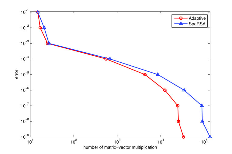
Fig. 1: Number of matrix-vector multiplications versus error

6.2 Image deblurring problems

In this subsection, we present results for two image restoration problems based on images referred to as Resolution and Cameraman. The images are $256\times 256$ gray scale images; that is, $n=256^{2}=65536$. The images are blurred by convolution with an $8\times 8$ blurring mask and normally distributed noise with standard deviation $0.0055$ is added to the final signal (see problem 701 in [21]). The image restoration problem has the form (2) where $\tau=0.00005$ and ${\bf{A}}={\bf{HW}}$ is the composition of the blur matrix and the Haar discrete wavelet transform (DWT) operator. For these test problems, the continuation approach is no faster, and in some cases significantly slower, than the implementation without continuation. Therefore, we solved these test problems without the continuation technique. The results in Table 2 again indicate that the adaptive scheme yields much better performance as the error tolerance decreases.

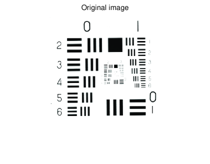
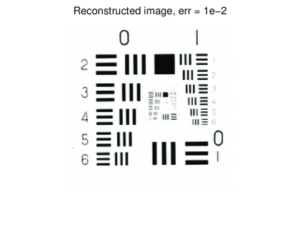
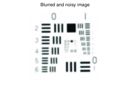
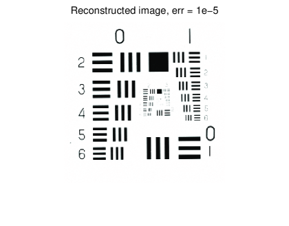
Fig. 2: Deblurring the resolution image

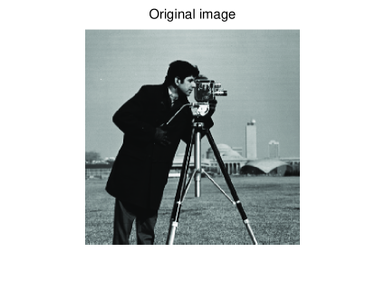
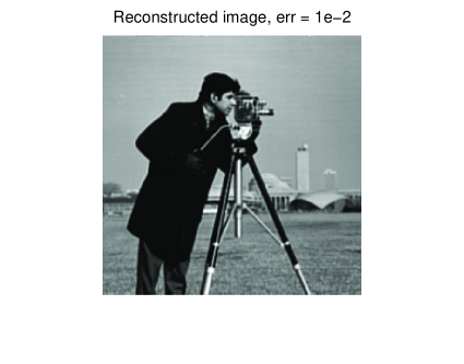
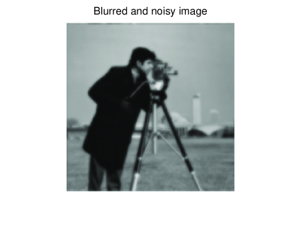
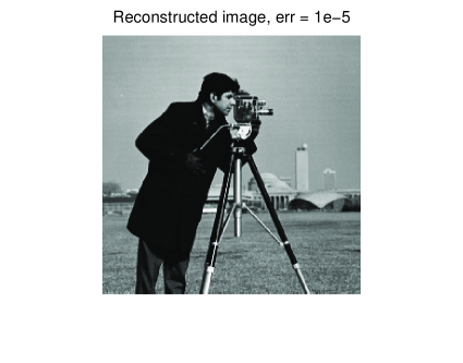
Fig. 3: Deblurring the cameraman image

Table 2: Deblurring images

error			1e-2			1e-3			1e-4			1e-5
	Ax	cpu	Obj	Ax	cpu	Obj	Ax	cpu	Obj	Ax	cpu	Obj
Resolution
SpaRSA	49	2.57	.4843	88	4.80	.3525	458	24.74	.2992	1679	88.27	.2970
Adaptive	37	1.93	.5619	73	4.02	.3790	316	17.28	.2981	681	35.90	.2970
Cameraman
SpaRSA	34	1.66	.3491	77	3.99	.2181	332	17.08	.1880	1356	69.45	.1868
Adaptive	35	1.71	.3380	63	3.31	.2232	215	11.20	.1880	599	31.4	.1868

6.3 Group-separable regularizer

In this subsection, we examine performance using the group separable regularizers [24] for which

$$\psi({\bf{x}})=\tau\sum_{i=1}^{n}\|{\bf{x}}_{[i]}\|_{2},$$

where ${\bf{x}}_{[1]},{\bf{x}}_{[2]},\ldots,{\bf{x}}_{[m]}$ are $m$ disjoint subvectors of ${\bf{x}}$. The smooth part of $\phi$ can be expressed as $f({\bf{x}})=\frac{1}{2}\|{\bf{A}}{\bf{x}}-{\bf{b}}\|^{2}$, where ${\bf{A}}\in\mathbb{R}^{1024\times 4096}$ was obtained by orthonormalizing the rows of a matrix constructed in Subsection 6.1. The true vector ${\bf{x}}_{true}$ has 4096 components divided into $m=64$ groups of length $l_{i}=64$. ${\bf{x}}_{true}$ is generated by randomly choosing 8 groups and filling them with numbers chosen from a Gaussian distribution with zero mean and unit variance, while all other groups are filled with zeros. The target vector is ${\bf{b}}={\bf{Ax}}_{true}+{\bf{n}}$, where ${\bf{n}}$ is Gaussian noise with mean zero and variance $10^{-4}$. The regularization parameter is chosen as suggested in [24]: $\tau=0.3\|{\bf{A}}^{\sf T}{\bf{b}}\|_{\infty}$. We ran 10 test problems with error tolerance $=10^{-5}$ and compute the average results. Adaptive SpaRSA solved the test problem in 0.8420 seconds with 67.4 matrix/vector multiplications, while the SpaRSA obtained similar performance: 0.8783 seconds and 69.1 matrix/vector multiplications. Figure 4 shows the result obtained by both methods for one sample.

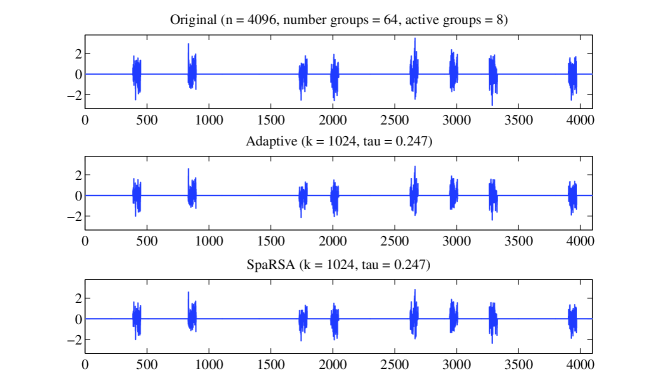
Fig. 4: Group-separable reconstruction

6.4 Total-variation phantom reconstruction

In this experiment, the image is the Shepp-Logan phantom of size $256\times 256$ (see [3, 5]). The objective function was

$$\phi({\bf{x}})=\frac{1}{2}\|{\bf{A}}({\bf{x}})-{\bf{b}}\|^{2}+.01\mbox{TV}({\bf{x}})$$

where ${\bf{A}}$ is a $6136\times 256^{2}$ matrix corresponding to 6136 locations in the 2D Fourier plane (masked_FFT in Matlab). The total variation (TV) regularization is defined as follows

$$\mbox{TV}({\bf{x}})=\sum_{i}\sqrt{\left(\triangle_{i}^{h}{\bf{x}}\right)^{2}+\left(\triangle_{i}^{v}{\bf{x}}\right)^{2}}$$

where $\triangle_{i}^{h}$ and $\triangle_{i}^{v}$ are linear operators corresponding to horizontal and vertical first order differences (see [4]). As seen in Table 3, Adaptive SpaRSA was faster than the original SpaRSA when the error tolerance was sufficiently small.

Table 3: Total-variation phantom reconstruction

error			1e-2			1e-3			1e-4
	Ax	cpu	Obj	Ax	cpu	Obj	Ax	cpu	Obj
SpaRSA	14	2.55	36.7311	143	30.06	14.7457	2877	938.25	14.1433
Adaptive	14	2.57	36.7311	136	27.32	14.6840	731	185.62	14.1730

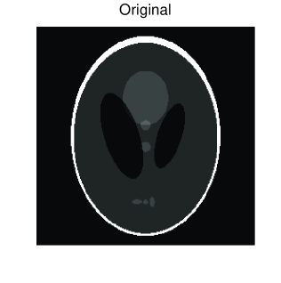
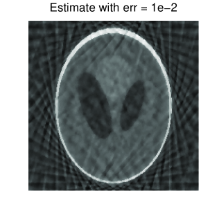
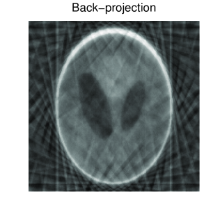
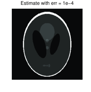
Fig. 5: Phantom reconstruction

7 Conclusions

The convergence properties of the SpaRSA algorithm (Sparse Reconstruction by Separable Approximation) of Wright, Nowak, and Figueiredo [24] are analyzed. We establish sublinear convergence when $\phi$ is convex and the GLL reference function value [14] is employed. When $\phi$ is strongly convex, the convergence is R-linear. For a reference function value which satisfies (R1)–(R3), we prove the existence of a convergent subsequence of iterates that approaches a stationary point. For a slightly stronger version of (R3), given in (27), we show that sublinear or linear convergence again hold when $\phi$ is convex or strongly convex respectively. In a series of numerical experiments, it is shown that an Adaptive SpaRSA, based on a relaxed choice of the reference function value and a cyclic BB iteration [9, 15], often yields much faster convergence, especially when the error tolerance is small.

References

- [1] J. Barzilai and J. M. Borwein, Two point step size gradient methods, IMA J. Numer. Anal., 8 (1988), pp. 141–148.
- [2] A. Beck and M. Teboulle, A fast iterative shrinkage-thresholding algorithm for linear inverse problems, SIAM Journal on Imaging Sciences, 2 (2009), pp. 183–202.
- [3] J. Bioucas-Dias and M. Figueiredo, Twist: Two-step iterative shrinkage/thresholding algorithm for linear inverse problems. http://www.lx.it.pt/bioucas/TwIST/TwIST.htm.
- [4] J. Bioucas-Dias, M. Figueiredo, and J. P. Oliveira, Total variation-based image deconvolution: a majorization-minimization approach., in Proceedings of the IEEE International Conference on Acoustics, Speech and Signal Processing, vol. 2, 2006, pp. 861–864.
- [5] E. J. Candès and J. Romberg, Practical signal recovery from random projections., Wavelet Applications in Signal and Image Processing XI, Proc. SPIE Conf., 5914 (2005).
- [6] A. Chambolle, R. A. DeVore, N. Y. Lee, and B. J. Lucier, Nonlinear wavelet image processing: Variational problems, compression, and noise removal through wavelet shrinkage, IEEE Trans. Image Process., 7 (1998), p. 319–335.
- [7] S. Chen, D. Donoho, and M. Saunders, Atomic decomposition by basis pursuit, SIAM J. Sci. Comput., 20 (1998), pp. 33–61.
- [8] Y. H. Dai, Alternate stepsize gradient method, Optimization, 52 (2003), pp. 395–415.
- [9] Y. H. Dai, W. W. Hager, K. Schittkowski, and H. Zhang, The cyclic Barzilai-Borwein method for unconstrained optimization, IMA J. Numer. Anal., 26 (2006), pp. 604–627.
- [10] I. Daubechies, M. Defrise, and C. D. Mol, An iterative thresholding algorithm for linear problems with a sparsity constraint, Comm. Pure Appl. Math., 57 (2004), pp. 1413–1457.
- [11] M. A. T. Figueiredo, R. D. Nowak, and S. J. Wright, Gradient projection for sparse reconstruction: Application to compressed sensing and other inverse problems, IEEE Journal on Selected Topics in Signal Processing, 1 (2007), pp. 586–597.
- [12] T. Figueiredo and R. D. Nowak, An EM algorithm for wavelet-based image restoration, IEEE Trans. Image Process., 12 (2003), p. 906–916.
- [13] A. Friedlander, J. M. Martínez, B. Molina, and M. Raydan, Gradient method with retards and generalizations, SIAM J. Numer. Anal., 36 (1999), pp. 275–289.
- [14] L. Grippo, F. Lampariello, and S. Lucidi, A nonmonotone line search technique for Newton’s method, SIAM J. Numer. Anal., 23 (1986), pp. 707–716.
- [15] W. W. Hager and H. Zhang, A new active set algorithm for box constrained optimization, SIAM J. Optim., 17 (2006), pp. 526–557.
- [16] E. Hale, W. Yin, and Y. Zhang, A fixed-point continuation method for -regularized minimization with applications to compressed sensing, tech. report, Rice University, July 2007.
- [17] S.-J. Kim, K. Koh, M. Lustig, S. Boyd, and D. Gorinevsky, An interior-point method for large-scale -regularized least squares, IEEE Journal on Selected Topics in Signal Processing, 1 (2007), pp. 606–617.
- [18] Y. Nesterov, Gradient methods for minimizing composite objective function, CORE Discussion Papers 2007/76, Université catholique de Louvain, Center for Operations Research and Econometrics (CORE), Sept. 2007.
- [19] M. Raydan and B. F. Svaiter, Relaxed steepest descent and Cauchy-Barzilai-Borwein method, Comput. Optim. Appl., 21 (2002), pp. 155–167.
- [20] R. T. Rockafellar, Convex analysis, Princeton Univ. Press, 1970.
- [21] E. van den Berg, M. P. Friedlander, G. Hennenfent, F. J. Herrmann, R. Saab, and O. Yilmaz, Algorithm 890: Sparco: A testing framework for sparse reconstruction, ACM Trans. Math. Softw., 35 (2009), pp. 1–16.
- [22] L. Vandenberghe, Gradient methods for nonsmooth problems (lecture note - spring 2009). http://www.ee.ucla.edu/vandenbe/ee236c.html.
- [23] C. Vonesch and M. Unser, Fast iterative thresholding algorithm for wavelet-regularized deconvolution, in Proceedings of the SPIE Optics and Photonics 2007 Conference on Mathematical Methods: Wavelet XII, vol. 6701, San Diego, CA, 2007, pp. 1–5.
- [24] S. J. Wright, R. D. Nowak, and M. A. T. Figueiredo, Sparse reconstruction by separable approximation, IEEE Trans. Signal Process., 57 (2009), pp. 2479–2493.