Particle kinematics in a dilute, 3-dimensional, vibration-fluidized granular medium

Abstract

We report an experimental study of particle kinematics in a 3-dimensional system of inelastic spheres fluidized by intense vibration. The motion of particles in the interior of the medium is tracked by high speed video imaging, yielding a spatially-resolved measurement of the velocity distribution. The distribution is wider than a Gaussian and broadens continuously with increasing volume fraction. The deviations from a Gaussian distribution for this boundary-driven system are different in sign and larger in magnitude than predictions for homogeneously driven systems. We also find correlations between velocity components which grow with increasing volume fraction.

The distribution of particle velocities is a fundamental descriptor of the statistics of a particulate system. In thermal equilibrium, this distribution is always a Boltzmann distribution, but that is typically not the case for a nonequilibrium steady state. An archetype of such a steady state is the inelastic gas, a system of particles that interact by dissipative contact forces, with the energy lost being compensated by a driving mechanism. Since the inelastic gas is both of fundamental interest and closely related to technologically important granular media, it has been the subject of much recent experimental, simulational and theoretical activityBarrat05 . Most experiments of inelastic gases have focused on 2-dimensional (2D) systems; in this article, we present the first detailed measurement of the velocity distribution in a fully 3-dimensional (3D) gas of inelastic grains.

Inelastic steady states may be broadly divided into systems driven from the boundaries and those that are driven homogeneously in the bulk. Homogeneously heated granular gases are represented theoretically by inelastically colliding particles energized by random, spatially homogeneous, uncorrelated boosts of energy between collisions. It has been shown Noije98 that the high-velocity tail of the velocity distribution for this model is of the form $P(c)\propto exp(-Ac^{3/2})$ where $c=v/\sigma$ is a velocity component, $v$ normalized by its r.m.s value $\sigma$. The velocity distribution for low velocities was computed by finding perturbative solutions to the Boltzmann equation in an expansion in Sonine polynomials around a Gaussian Goldshtein95 ; Noije98 . In both limits, the results depend on inelasticity but not on volume fraction, $\phi$. These results have been confirmed by simulationBrey96 ; Monterato00 ; Moon01 . The closest experimental analogues for this model are 2D monolayers of particles fluidized by a vibrated baseLosert99 where velocity distributions depend strongly on the nature of the basePrevost02 ; for a sufficiently rough base Shattuck07 , the Sonine expansion describes the distribution satisfactorily. There are no 3D realizations of the homogeneously heated granular gas with random forcing in the bulk of the medium.

Much less theoretical effort has been directed toward the more naturally prevalent boundary-driven system. On the other hand, several experiments have studied 2D systems driven by vibration Menon00 ; Kudrolli00 and electrostatic driving Olafsen02 . Some experiments Menon00 ; Olafsen02 show the entire distribution of velocity fluctuations can be described by the functional form $P(c)\!\propto\!exp(-Ac^{\beta})$ with $\beta\approx\frac{3}{2}$ over a broad range of number density and inelasticity. The relationship of these experimental results to the prediction of Noije98 are unclear since simulations of the homogeneously heated gas Barrat03 show that the asymptotic high-velocity behavior only sets in extremely deep in the tail, too rare to be experimentally detectable. Furthermore, the measured distribution differs between experiments, possibly because these quasi-2D experiments are sensitive to the specifics of the confinement in the thin dimension Menon00 ; Olafsen04 ; vanZon04 or to the substrate on which they move Kudrolli00 .

Three-dimensional steady states have been much less studied due to the challenges of tracking particles in the interior of a system. Two techniques that have been employed for 3D vibrated systems are positron emission tracking Wildman01 of tracer particles, and nuclear magnetic resonance imaging Huan04 . These studies focused on spatial profiles of temperature and number density, although a non-Gaussian velocity distribution was reported by the NMR technique Huan04 . Simulations show Brey03 ; Barrat04 ; Moon04 ; Zippelius04 ; MacKintosh that the velocity distribution evolves continuously from a nearly-Gaussian distribution to $P(c)\!\sim\!exp(-Ac^{\beta})$. There are no direct predictions for boundary-driven systems, but models MacKintosh ; Machta05 which vary $q$, the ratio of the frequency of particle collisions to the frequency of heating events, give some intuition on the passage from the homogeneously heated ($q\!\approx\!1$) to the boundary-driven ($q\!\gg\!1$) case.

In this article we describe experiments using high-speed video imaging to directly locate and track particles in the bulk of a 3D vibration-fluidized steady state. We report kinetic temperature profiles, the form of velocity distribution, and comparisons with available predictions.

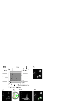
Figure 1: (a) Sketch of the experimental setup. A cubical cell is driven vertically by a shaker. The shaded rectangle is a plane of thickness $1d$ illuminated by laser sheets from both sides. The darker shading shows the area imaged by the camera. (b) Part of a video frame. (c) Edge detection performed on this frame. (d) Illustration of the rays emanating from the edge, along the intensity gradient, for the top right particle in (b). The solid rays converge toward the center and dashed rays diverge. (e) Surface plot for these accumulated gradient rays. (f) Located particle positions. For the value of the threshold applied to the peaks in (e), the fourth particle in the frame is not located.

As shown in Fig.1(a), a cubical cell with acrylic vertical walls is sinusoidally vibrated in the vertical direction by an electromechanical shaker (Ling Dynamics V456). The vibration frequency used in the experiment ranges from 50Hz to 80Hz, velocity amplitudes $V_{0}$ from 2.3 m/s to 3.7 m/s, and accelerations from 90$g$ to 190$g$. The bottom and top walls are rough glass plates that provide a low-inelasticity surface but also randomise the direction of collisional momentum transfer. We use delrin spheres of diameter $d=1.560\pm 0.003$mm and an average normal coefficient of restitution $\varepsilon=0.92\pm 0.21$, experimentally determined from particle collisions. The error bar reflects the dependence of $\varepsilon$ on impact parameter, relative particle velocity, and spin. The side of the cell is $51.2$mm $\approx 32d$ and is illuminated by light sheets produced by expanding beams from laser diodes (Thorlabs ML101J8) with a cylindrical lens. The thickness of the sheet in the $y$-direction is $\approx\!1d$, and its $y$-position can be varied, allowing us to study particle motions in $x$-$z$ planes at varying depth from the front wall. A Phantom v7 camera images the $x$-$z$ plane selected by the light sheet, at 5,000 frames/second, with a resolution of $640\times 480$ pixels. The field of view is a rectangle of width $\approx 30d$ and height $20d$, centred on the middle of the cell.

The difficulty in locating particles stems from two distinct eclipsing effects. First, particles in the middle of the cell are less likely to be illuminated because the light-sheet is obstructed by particles in the light path. The delrin spheres are homogeneously illuminated; any laser light incident on a sphere is scattered through its volume. However, when the light-sheet is at some depth from the front plane, illuminated spheres can be partially eclipsed by particles in front of them. We focus on velocity statistics rather than number density distributions since the detection probability of a particle depends on these two effects. A video frame with examples of partially eclipsed particles is shown in Fig.1b. To locate particles, we exploit the fact that the convex illuminated edges of the images are circular arcs of known radius. We find illuminated edges (Fig.1c) and draw rays from all edge points in the direction of the local intensity gradient. For points on convex illuminated edges, these rays converge to the centre, while concave edges produce rays that diverge (Fig.1d). Local maxima for accumulations of rays (Fig.1e) above a cut-off value are candidates for particle centres; objects with an insufficient length of illuminated perimeter are rejected. Particle centres are determined with subpixel resolution by minimising the squared distance to the gradient rays. Eclipsing produces no systematic bias in locating particle centres.

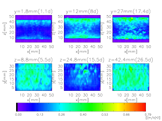
Figure 2: Distribution of the kinetic temperature at planes of various $y$(top row) and $z$(lower row). The dashed line shows the midplane of the cell. The driving frequency is 60Hz, $\Gamma=110g$ and volume fraction 5.1%.

The kinetic temperature $T=\frac{1}{2}(\left<v_{x}^{2}\right>+\left<v_{z}^{2}\right>)$ is measured at several depths, $y$, between the front plane and a little beyond the middle of the cell. As shown in Fig.2 (top row), in any given $x$-$z$ plane, $T$ is higher near the top and bottom wall, and lower in the middle. Comparing $x$-$z$ planes at different depths $y$, we see that $T$ goes up in the middle of the cell, revealing the dissipative effect of the front vertical wall. The data are then reorganized to show $T(x,y)$ at a few heights, $z$ (Fig.2 bottom row). Within each plane, $T$ is lower close to the vertical walls, again due to the dissipation at the walls. The length scale over which the wall dissipation manifests itself is comparable to the mean free path, and grows at lower $\phi$.

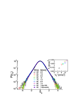
Figure 3: $P(c_{x})$ for $\phi=5.1\%$ for various driving frequencies and amplitudes, sampled at $y=8d$. One data set taken with smooth top and bottom plates, and another set taken at $y=3d$ are included for comparison. The inset shows the average kinetic temperature of the sampled region as a function of $V_{0}^{2}$, where $V_{0}$ is the amplitude of the driving velocity.

We now turn to the entire distribution of the velocity fluctuations. The velocity fluctuations are anisotropic; we concentrate on $v_{x}$, the horizontal component, perpendicular to the driving direction. The distribution $P(c_{x})$ of $c_{x}$, the normalized horizontal velocity $c_{x}=v_{x}/(2T_{x})^{1/2}$ where $T_{x}=\left<v_{x}^{2}\right>$, shows weak dependence on position very close to the walls of the cell (as also seen in simulations Barrat04 ; Moon04 ). Therefore, we report data at $y=8d$ which is far from the front wall, and yet not so deep in the cell where the velocity statistics are greatly diminished by eclipsing effects. The dependence of $P(c_{x})$ on different driving frequencies and amplitude is shown in Fig.3. As the overall temperature is changed by a factor of 3, we observe no systematic changes in $P(c_{x})$. In experiments on 2D monolayers Shattuck07 ; Prevost02 it was noted that velocity distribution depended on the smoothness of the driving surface, as might be expected when interparticle collisions and heating events occur with comparable frequency. To test whether the influence of the boundary persists into the interior, we replace the rough glass plates by smooth delrin plates and do not observe any change in $P(c_{x})$. This suggests that the observed statistics are a consequence of inter-particle collisions, and are insensitive to the details of the driving surface.

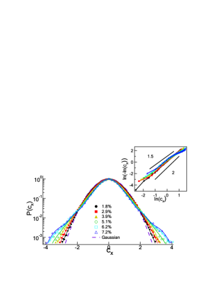
Figure 4: $P(c_{x})$, different volume fractions ranging from 1.8% to 7.2%. The smooth lines connecting symbols are a guide to the eye. The inset shows $ln(-ln(c_{x}))$ vs $ln(c_{x})$.

Having established that distribution of horizontal velocities is insensitive to $T$, to the driving surface, and to location within the cell, we now discuss the dependence of $P(c_{x})$ on the number density of particles. We have studied six volume fractions $\phi$ ranging from 1.8 to 7.2%. The lower limit on $\phi$ is chosen so that the mean free path is still much smaller than the cell dimensions, and the upper limit is constrained by poor detection statistics at high volume fractions. Deviations from a Gaussian are apparent even at the lowest $\phi$. With increasing $\phi$, the tails of $P(c_{x})$ get broader. Thus the velocity distribution varies continuously with density unlike in some 2D experiments Menon00 ; Olafsen04 where $P(c_{x})$ is unchanged over a broad range of $\phi$. This is also unlike predictions for the homogeneously driven or cooled state Noije98 where $P(c)$ is independent of $\phi$.

The high-velocity tail of $P(c_{x})$ cannot be described by the form $exp(-c_{x}^{\beta})$: as shown in the inset of Fig.4, a plot of $ln(-lnP(c_{x}))$ against $ln(c_{x})$, shows curvature, whereas in the equivalent 2D experimentMenon00 we observed a straight line with a slope $\beta=1.55\pm 0.1$. The statistics in the experiment only capture the tail up to 4 decades below the peak, and leave open the possibility that this could be the asymptotic form of the distribution at large $c$. However, for any realistic description of grain dynamics, even rarer fluctuations are probably irrelevant. Earlier simulationsBrey03 ; Barrat04 ; Moon04 ; Zippelius04 ; MacKintosh have found density-dependent velocity distributions, however, this is the first experimental study in 3D to observe this effect.

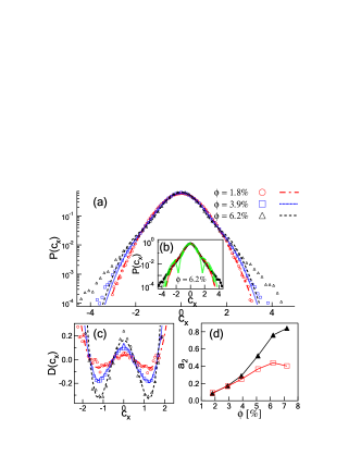
Figure 5: (a)$P(c_{x})$ at volume fractions $\phi=1.8,3.9$ and $6.2\%$ fitted to second-order Sonine polynomials with $a_{2}$ treated as a free parameter. (b)$P(c_{x})$ at volume fraction $\phi=6.2\%$ with best fit second- (red dash line, $a_{2}=0.440$) and third-order (red dotted line, $a_{2}$ = 0.455, $a_{3}$ = -0.0287) Sonine forms. The green dashed and dotted lines show the 2nd and 3rd order Sonine forms with the coefficients $a_{2}$ and $a_{3}$ computed from the measured cumulants. (c)The deviation function $D(c_{x})$ at small $c_{x}$ for the above volume fractions. (d)The best fit value of $a_{2}$ ($\blacktriangle$) compared with $a_{2}$ ($\square$) computed from $\left<c^{4}\right>$.

In the absence of predictions for the a boundary-driven system, we compare $P(c)$ to predictions for a homogeneously heated inelastic gas, where at small velocities, the deviations $D(c)$ from the gaussian distribution, $\Phi(c)$, have been perturbatively calculated Goldshtein95 ; Noije98 as an expansion in Sonine polynomials $S_{p}(c^{2})$ :

$$P(c)=\Phi(c)\left[1+D(c)\right]=\Phi(c)\left[1+\sum_{p=1}^{\infty}a_{p}S_{p}\left(c^{2}\right)\right]\,.$$ (1)

The first two polynomials are $S_{1}(c^{2})=-c^{2}+\frac{1}{2}\hat{d}$ and $S_{2}(c^{2})=\frac{1}{2}c^{4}-\frac{1}{2}(\hat{d}+2)c^{2}+\frac{1}{8}\hat{d}(\hat{d}+2)$ where $\hat{d}$ is the dimensionality. The coefficients $a_{p}$ are given in terms of the moments of the distribution, $P(c)$: $a_{1}=0,a_{2}=4\left<c^{4}\right>/(\hat{d}(\hat{d}+2))-1$. Predictions Noije98 for the dependence of $a_{2}$ on the restitution coefficient for the homogeneously heated and cooling states have been validated by both DSMC and event-driven simulationsBrey96 ; Monterato00 ; Moon01 . In Fig.5 we test whether the Sonine expansion is a good description of $P(c_{x})$ in our boundary driven system by fitting the data for varying volume fraction to a second-order Sonine expansion with $a_{2}$ as a free parameter.

Fig.5(a)-(c) show that the second-order Sonine correction works best at the lowest volume fraction and the range over which $D(c)$, the deviation from a gaussian, is well-fit diminishes at higher volume fractions. As in the quasi-2D experiment of Shattuck07 which models a homogeneously heated gas; the quality of the fit is reasonable for $c\lesssim 2$.A third-order Sonine term does not improve the fit, as shown in Fig.5(b).

Apart from the dependence on $\phi$ of the fit parameter $a_{2}$, we also note that $a_{2}$ is opposite in sign, and much larger in magnitude than that found in the homogeneously heated or cooled states for the same nominal restitution coefficient. Furthermore, as shown in Fig.5(d) the best-fit value of $a_{2}$ disagrees with the value directly calculated from the 4th cumulant, $\left<c^{4}\right>$, raising the possibility that the gaussian reference state may not be appropriate for a boundary-driven system. To our knowledge, the only predictions for P(c) in a boundary-driven system were made in Risso02 , where the 4th cumulant is treated as an independent hydrodynamic field. They find $\left<c^{4}\right>$ shows a density dependence qualitatively like ours, but with much lower magnitude than we measure.

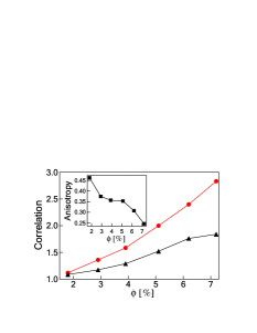
Figure 6: The correlation of $v_{x}$ and $v_{z}$ ($\bullet$), and the correlation implicit in the Sonine formula($\blacktriangle$): $1+a_{2}$. The inset shows the anisotropy, $(v_{z}^{2}-v_{x}^{2})/(v_{x}^{2}+v_{z}^{2})$.

A general consideration regarding $P(c)$ is that if a velocity distribution is isotropic and if the velocity components are uncorrelated, it must be a gaussian distribution. A non-gaussian distribution implies that one or both of these assumptions is invalid. For low volume fractions, the velocity fluctuations are anisotropic, but they become more isotropic at higher densities. This trend is shown in the inset to Fig.6 where the anisotropy is quantified by $2\left<v_{z}^{2}-v_{x}^{2}\right>/\left<v_{z}^{2}+v_{x}^{2}\right>$. However, since the velocity distribution does not tend towards a Gaussian at large $\phi$, the velocity components must be correlated as shown in Fig.6. Indeed, the correlation between velocity components $\left<v_{x}^{2}v_{z}^{2}\right>/\left<v_{x}^{2}\right>\left<v_{z}^{2}\right>$ grows with volume fraction $\phi$.

Our measurements of the 3D particle kinematics in the interior of a vibration-fluidized granular medium thus reveal a non-Gaussian velocity distribution that is insensitive to conditions at the driving surface. The shape of the distribution evolves continuously with volume fraction; the functional form differs markedly from the homogeneously heated state, thus emphasizing the need for theoretical development for boundary-driven systems.

We are grateful for support through NASA NNC05AA35A and NSF-DMR0606216, and to R. Soto, M.D. Shattuck, J.L. Machta for valuable comments.

References

- (1) A.Barrat, E.Trizac, M.H.Ernst, J. Phys.:Condens.Matter 17, S2429(2005).
- (2) T.P.C. van Noije, M.H.Ernst, Granular Matter 2, 57(1998).
- (3) A.Goldshtein, M.Shapiro, J. Fluid Mech. 282, 75(1995).
- (4) J.J.Brey, M.J.Ruiz-Montero, D.Cubero, Phys. Rev. E 54, 3664(1996).
- (5) J.M.Montanero, A.Santos, Granular Matter 2, 53(2000).
- (6) S.J.Moon, M.D.Shattuck, J.B.Swift, Phys. Rev. E 64, 031303(2001).
- (7) W.Losert et al., Chaos, 9, 682(1999).
- (8) A.Prevost, D.A.Egolf, J.S.Urbach, Phys. Rev. Lett.,89, 084301(2002).
- (9) P.M.Reis, R.A.Ingale, M.D.Shattuck, Phys. Rev. E 75, 051311(2007).
- (10) F.Rouyer, N.Menon, Phys. Rev. Lett. 85, 3676(2000).
- (11) A.Kudrolli, J.Henry, Phys. Rev. E 62, R1489(2000).
- (12) I.S.Aranson, J.S.Olafsen, Phys. Rev. E 66, 061302(2002).
- (13) A.Barrat, E.Trizac, Eur. Phys. J. E 11, 99(2003).
- (14) G.W.Baxter, J.S.Olafsen, Nature 425, 680(2004).
- (15) J.S.van Zon et al., Phys. Rev. E 70, 040301(R)(2004).
- (16) R.D.Wildman, J.M.Huntley, and D.J.Parker, Phys. Rev. E 63, 061311(2001).
- (17) C.Huan et al., Phys. Rev. E 69, 041302(2004).
- (18) J.J.Brey, M.J.Ruiz-Montero, Phys. Rev. E 67, 021307(2003).
- (19) A.Barrat, E.Trizac, Phys. Rev. E 66, 051303(2002).
- (20) S.J.Moon, J.B.Swift, H.L.Swinney, Phys. Rev. E 69, 011301(2004).
- (21) O.Herbst, P. Müller, M.Otto, A.Zippelius, Phys. Rev. E 70, 051313(2004).
- (22) J.S.van Zon, F.C.MacKintosh, Phys. Rev. Lett. 93, 038001(2004); Phys. Rev. E 72, 051301(2005).
- (23) E.Ben-Naim, J.Machta, Phys. Rev. Lett. 94, 138001(2005).
- (24) D.Risso, P.Cordero, Phys. Rev. E 65, 021304(2002).
- (25) N.V.Brilliantov, T.Pöschel, Europhys. Lett. 74, 424(2006).