Abstract

In this article, we re-study the heavy baryon states $\Omega_{b}$, $\Omega_{c}$, $\Xi^{\prime}_{b}$, $\Xi^{\prime}_{c}$, $\Sigma_{b}$ and $\Sigma_{c}$ with the QCD sum rules, after subtracting the contributions from the corresponding negative parity heavy baryon states, the predicted masses are in good agreement with the experimental data.

PACS number: 14.20.Lq, 14.20.Mr

Key words: Heavy baryon states, QCD sum rules

1 Introduction

The charm and bottom baryons which contain a heavy quark and two light quarks are particularly interesting for studying dynamics of the light quarks in the presence of a heavy quark, and serve as an excellent ground for testing predictions of the constituent quark models and heavy quark symmetry. The ${1\over 2}^{+}$ antitriplet states ($\Lambda_{c}^{+}$, $\Xi_{c}^{+},\Xi_{c}^{0})$, and the ${1\over 2}^{+}$ and ${3\over 2}^{+}$ sextet states ($\Omega_{c},\Sigma_{c},\Xi^{\prime}_{c}$) and ($\Omega_{c}^{*},\Sigma_{c}^{*},\Xi^{*}_{c}$) have been established; while the corresponding bottom baryons are far from complete, only the $\Lambda_{b}$, $\Sigma_{b}$, $\Sigma_{b}^{*}$, $\Xi_{b}$ and $\Omega_{b}$ have been observed [1].

The QCD sum rules is a powerful theoretical tool in studying the ground state heavy baryons [2, 3]. The masses of the $\Lambda_{Q}$, $\Sigma_{Q}$, $\Xi_{Q}$, $\Xi^{\prime}_{Q}$, $\Omega_{Q}$, $\Sigma^{*}_{Q}$, $\Xi^{*}_{Q}$ and $\Omega^{*}_{Q}$ have been calculated with the full QCD sum rules [4, 5, 7, 8, 9, 10, 11, 12]. The masses of the $\Sigma^{*}_{Q}$, $\Sigma_{Q}$ and $\Lambda_{Q}$ have been calculated with the QCD sum rules in the leading order of the heavy quark effective theory [13, 14, 15], and later the $1/m_{Q}$ corrections were studied [16, 17, 18]. Furthermore, the masses of the orbitally excited heavy baryons with the leading order approximation [19, 20], and the $1/m_{Q}$ corrections [21] in the heavy quark effective theory have also been analyzed. Recently the $\frac{1}{2}^{+}$ and $\frac{3}{2}^{+}$ bottom baryon states were studied with the QCD sum rules in the heavy quark effective theory including the $1/m_{Q}$ corrections [22].

In 2008, the D0 collaboration reported the first observation of the doubly strange baryon $\Omega_{b}^{-}$ in the decay channel $\Omega_{b}^{-}\to J/\psi\thinspace\Omega^{-}$ (with $J/\psi\to\mu^{+}\mu^{-}$ and $\Omega^{-}\to\Lambda K^{-}\to p\pi^{-}K^{-}$) in $p\bar{p}$ collisions at $\sqrt{s}=1.96$ TeV [23]. The experimental value $M_{\Omega_{b}^{-}}=6.165\pm 0.010\thinspace\pm 0.013\thinspace\,\rm{GeV}$ is about $0.1\,\rm{GeV}$ larger than the most theoretical calculations [24, 25, 26, 27, 28, 29, 30, 31, 22, 32]. However, the CDF collaboration did not confirm the measured mass [33], i.e. they observed the mass of the $\Omega^{-}_{b}$ is about $6.0544\pm 0.0068\pm 0.0009\,\rm{GeV}$, which is consistent with the most theoretical calculations. On the other hand, the theoretical prediction $M_{\Omega_{c}^{0}}\approx 2.7\,\rm{GeV}$ [24, 25, 26, 27, 28, 29, 30, 31, 22, 32, 34] is consistent with the experimental data $M_{\Omega_{c}^{0}}=(2.6975\pm 0.0026)\,\rm{GeV}$ [1].

In Ref.[35], Jido et al introduce a novel approach based on the QCD sum rules to separate the contributions of the negative-parity light flavor baryons from the positive-parity light flavor baryons, as the interpolating currents may have non-vanishing couplings to both the negative- and positive-parity baryons [36]. In Ref.[15], Bagan et al take the infinite mass limit for the heavy quarks to separate the contributions of the positive and negative parity heavy baryon states to the correlation functions unambiguously before the work of Jido et al. In this article, we re-study the masses and pole residues of the ${\frac{1}{2}}^{+}$ heavy baryon states $\Omega_{Q}$, $\Xi^{\prime}_{Q}$ and $\Sigma_{Q}$ by subtracting the contributions from the negative parity baryon states. In Refs.[6, 11, 12], we study the ${\frac{1}{2}}^{+}$ heavy baryons $\Omega_{Q}$, $\Xi^{\prime}_{Q}$ and $\Sigma_{Q}$ and ${\frac{3}{2}}^{+}$ heavy baryons $\Omega_{Q}^{*}$, $\Xi^{*}_{Q}$ and $\Sigma^{*}_{Q}$ with the QCD sum rules in full QCD, and observe that the pole residues of the ${\frac{3}{2}}^{+}$ heavy baryons from the sum rules with different tensor structures are consistent with each other, while the pole residues of the ${\frac{1}{2}}^{+}$ heavy baryons from the sum rules with different tensor structures differ from each other greatly. Those pole residues are important parameters in studying the radiative decays $\Omega_{Q}^{*}\to\Omega_{Q}\gamma$, $\Xi_{Q}^{*}\to\Xi^{\prime}_{Q}\gamma$ and $\Sigma_{Q}^{*}\to\Sigma_{Q}\gamma$ [12, 37], we should refine those parameters to improve the predictive ability.

The article is arranged as follows: we derive the QCD sum rules for the masses and the pole residues of the heavy baryon states $\Omega_{Q}$, $\Xi^{\prime}_{Q}$ and $\Sigma_{Q}$ in section 2; in section 3 numerical results are given and discussed, and section 4 is reserved for conclusion.

2 QCD sum rules for the $\Omega_{Q}$, $\Xi^{\prime}_{Q}$ and $\Sigma_{Q}$

The ${\frac{1}{2}}^{+}$ heavy baryons $\Omega_{Q}$, $\Xi^{\prime}_{Q}$ and $\Sigma_{Q}$ can be interpolated by the following currents $J_{\Omega}(x)$, $J_{\Xi}(x)$ and $J_{\Sigma}(x)$ respectively,

$$J_{\Omega}(x) = \epsilon^{ijk}s^{T}_{i}(x)C\gamma_{\mu}s_{j}(x)\gamma_{5}\gamma^{\mu}Q_{k}(x)\,,$$

$$J_{\Xi}(x) = \epsilon^{ijk}q^{T}_{i}(x)C\gamma_{\mu}s_{j}(x)\gamma_{5}\gamma^{\mu}Q_{k}(x)\,,$$

$$J_{\Sigma}(x) = \epsilon^{ijk}u^{T}_{i}(x)C\gamma_{\mu}d_{j}(x)\gamma_{5}\gamma^{\mu}Q_{k}(x)\,,$$ (1)

where the $Q$ represents the heavy quarks $c$ and $b$, the $i$, $j$ and $k$ are color indexes, and the $C$ is the charge conjunction matrix. In this article, we take the simple Ioffe type interpolating currents, which are constructed by considering the diquark theory and the heavy quark symmetry [38, 39].

The corresponding negative-parity heavy baryon states can be interpolated by the currents $J_{-}=i\gamma_{5}J_{+}$ because multiplying $i\gamma_{5}$ to $J_{+}$ changes the parity of $J_{+}$ [35], where the $J_{+}$ denotes the currents $J_{\Omega}(x)$, $J_{\Xi}(x)$ and $J_{\Sigma}(x)$. The correlation functions are defined by

$$\Pi_{\pm}(p) = i\int d^{4}xe^{ip\cdot x}\langle 0|T\left\{J_{\pm}(x)\bar{J}_{\pm}(0)\right\}|0\rangle\,,$$ (2)

and can be decomposed as

$$\Pi_{\pm}(p)=\!\not\!{p}\Pi_{1}(p^{2})\pm\Pi_{0}(p^{2})\,,$$ (3)

due to Lorentz covariance, because

$$\Pi_{-}(p)=-\gamma_{5}\Pi_{+}(p)\gamma_{5}\,.$$ (4)

The currents $J_{+}$ couple to both the positive- and negative-parity baryons [36],

$$\langle{0}|J_{+}|B^{-}\rangle\langle B^{-}|\bar{J}_{+}|0\rangle=-\gamma_{5}\langle 0|J_{-}|B^{-}\rangle\langle B^{-}|\bar{J}_{-}|0\rangle\gamma_{5}\,,$$ (5)

where the $B^{-}$ denote the negative parity baryon states.

We insert a complete set of intermediate baryon states with the same quantum numbers as the current operators $J_{+}(x)$ and $J_{-}(x)$ into the correlation functions $\Pi_{+}(p)$ to obtain the hadronic representation [2, 3]. After isolating the pole terms of the lowest states, we obtain the following result [35]:

$$\Pi_{+}(p) = \lambda_{+}^{2}{\!\not\!{p}+M_{+}\over M^{2}_{+}-p^{2}}+\lambda_{-}^{2}{\!\not\!{p}-M_{-}\over M_{-}^{2}-p^{2}}+\cdots\,,$$ (6)

where the $M_{\pm}$ are the masses of the lowest states with parity $\pm$ respectively, and the $\lambda_{\pm}$ are the corresponding pole residues (or couplings). If we take $\vec{p}=0$, then

$$\rm{limit}_{\epsilon\rightarrow 0}\frac{{\rm Im}\Pi_{+}(p_{0}+i\epsilon)}{\pi} = \lambda_{+}^{2}{\gamma_{0}+1\over 2}\delta(p_{0}-M_{+})+\lambda_{-}^{2}{\gamma_{0}-1\over 2}\delta(p_{0}-M_{-})+\cdots$$ (7)

$$= \gamma_{0}A(p_{0})+B(p_{0})+\cdots\,,$$

where

$$A(p_{0}) = {1\over 2}\left[\lambda_{+}^{2}\delta(p_{0}-M_{+})+\lambda_{-}^{2}\delta(p_{0}-M_{-})\right]\,,$$

$$B(p_{0}) = {1\over 2}\left[\lambda_{+}^{2}\delta(p_{0}-M_{+})-\lambda_{-}^{2}\delta(p_{0}-M_{-})\right]\,,$$ (8)

the contribution $A(p_{0})+B(p_{0})$ ($A(p_{0})-B(p_{0})$) contains contributions from the positive parity (negative parity) states only.

We carry out the operator product expansion at large $Q^{2}(=-p_{0}^{2})$ region, then use the dispersion relation to obtain the spectral densities $\rho^{A}(p_{0})$ and $\rho^{B}(p_{0})$ (which correspond to the tensor structures $\gamma_{0}$ and $1$ respectively) at the level of quark-gluon degrees of freedom, finally we introduce the weight functions $\exp\left[-\frac{p_{0}^{2}}{T^{2}}\right]$, $p_{0}^{2}\exp\left[-\frac{p_{0}^{2}}{T^{2}}\right]$, and obtain the following sum rules,

$$\int_{\Delta}^{\sqrt{s_{0}}}dp_{0}\left[A(p_{0})+B(p_{0})\right]\exp\left[-\frac{p_{0}^{2}}{T^{2}}\right] = \int_{\Delta}^{\sqrt{s_{0}}}dp_{0}\left[\rho^{A}(p_{0})+\rho^{B}(p_{0})\right]\exp\left[-\frac{p_{0}^{2}}{T^{2}}\right]\,,$$

$$\int_{\Delta}^{\sqrt{s_{0}}}dp_{0}\left[A(p_{0})+B(p_{0})\right]p_{0}^{2}\exp\left[-\frac{p_{0}^{2}}{T^{2}}\right] = \int_{\Delta}^{\sqrt{s_{0}}}dp_{0}\left[\rho^{A}(p_{0})+\rho^{B}(p_{0})\right]p_{0}^{2}\exp\left[-\frac{p_{0}^{2}}{T^{2}}\right]\,,$$

where the $s_{0}$ are the threshold parameters, $T^{2}$ is the Borel parameter, $\Delta=m_{Q}+2m_{s}$, $\Delta=m_{Q}+m_{s}$ and $\Delta=m_{Q}$ in the channels $\Omega_{Q}$, $\Xi^{\prime}_{Q}$ and $\Sigma_{Q}$ respectively, the explicit expressions of the spectral densities $\rho^{A}(p_{0})$ and $\rho^{B}(p_{0})$ in the channels $\Omega_{Q}$, $\Xi^{\prime}_{Q}$ and $\Sigma_{Q}$ are presented in the appendix. In calculation, we take assumption of vacuum saturation for the high dimension vacuum condensates, they are always factorized to lower condensates with vacuum saturation in the QCD sum rules, and factorization works well in large $N_{c}$ limit. In this article, we take into account the contributions from the quark condensates, mixed condensates, gluon condensate, and neglect the contributions from other high dimension condensates, which are suppressed by large denominators and would not play significant roles.

3 Numerical results and discussions

The input parameters are taken to be the standard values $\langle\bar{q}q\rangle=-(0.24\pm 0.01\,\rm{GeV})^{3}$, $\langle\bar{s}s\rangle=(0.8\pm 0.2)\langle\bar{q}q\rangle$, $\langle\bar{q}g_{s}\sigma Gq\rangle=m_{0}^{2}\langle\bar{q}q\rangle$, $\langle\bar{s}g_{s}\sigma Gs\rangle=m_{0}^{2}\langle\bar{s}s\rangle$, $m_{0}^{2}=(0.8\pm 0.2)\,\rm{GeV}^{2}$ [40, 41], $\langle\frac{\alpha_{s}GG}{\pi}\rangle=(0.012\pm 0.004)\,\rm{GeV}^{4}$ [41], $m_{s}=(0.14\pm 0.01)\,\rm{GeV}$, $m_{c}=(1.35\pm 0.10)\,\rm{GeV}$ and $m_{b}=(4.7\pm 0.1)\,\rm{GeV}$ [1] at the energy scale $\mu=1\,\rm{GeV}$.

Those vacuum condensates can be calculated with lattice QCD and instanton models, or determined by fitting certain QCD sum rules to the experimental data; the values are consistent with each other (except for the gluon condensate $\langle\frac{\alpha_{s}GG}{\pi}\rangle$) considering the uncertainties. The value of the gluon condensate $\langle\frac{\alpha_{s}GG}{\pi}\rangle$ has been updated from time to time, and changes greatly (for a comprehensive review, one can consult the book ”QCD as a theory of hadrons from partons to confinement” by S.Narison [42]). At the present case, the gluon condensate makes tiny contribution, the updated value $\langle\frac{\alpha_{s}GG}{\pi}\rangle=(0.023\pm 0.003)\,\rm{GeV}^{4}$ [42] and the standard value $\langle\frac{\alpha_{s}GG}{\pi}\rangle=(0.012\pm 0.004)\,\rm{GeV}^{4}$ [41] lead to a difference less than $2\,\rm{MeV}$ for the masses.

The $Q$-quark masses appearing in the perturbative terms (see the appendix) are usually taken to be the pole masses in the QCD sum rules, while the choice of the $m_{Q}$ in the leading-order coefficients of the higher-dimensional terms is arbitrary [42, 43]. For example, the $\overline{MS}$ mass $m_{c}(m_{c}^{2})$ relates with the pole mass $\hat{m}$ through the relation

$$m_{c}(m_{c}^{2}) = \hat{m}\left[1+\frac{C_{F}\alpha_{s}(m_{c}^{2})}{\pi}+(K-2C_{F})\left(\frac{\alpha_{s}}{\pi}\right)^{2}+\cdots\right]^{-1}\,,$$ (11)

where $K$ depends on the flavor number $n_{f}$. In this article, we take the approximation $m_{c}\approx\hat{m}$ without the $\alpha_{s}$ corrections for consistency. The value listed in the Particle Data Group is $m_{c}(m_{c}^{2})=1.27^{+0.07}_{-0.11}\,\rm{GeV}$ [1], it is reasonable to take the value $m_{c}=m_{c}(1\,\rm{GeV}^{2})=(1.35\pm 0.10)\,\rm{GeV}$ in our works. The mass of the $b$ quark $m_{b}$ can be understood analogously.

In calculation, we also neglect the contributions from the perturbative corrections $\mathcal{O}(\alpha_{s}^{n})$. Those perturbative corrections can be taken into account in the leading logarithmic approximations through anomalous dimension factors. After the Borel transform, the effects of those corrections are to multiply each term on the operator product expansion side by the factor,

$$\left[\frac{\alpha_{s}(T^{2})}{\alpha_{s}(\mu^{2})}\right]^{2\Gamma_{J}-\Gamma_{\mathcal{O}_{n}}}\,,$$ (12)

where the $\Gamma_{J}$ is the anomalous dimension of the interpolating current $J(x)$, the $\Gamma_{\mathcal{O}_{n}}$ is the anomalous dimension of the local operator $\mathcal{O}_{n}(0)$ in the operator product expansion,

$$T\left\{J(x)J^{\dagger}(0)\right\} = C_{n}(x){O}_{n}(0)\,,$$ (13)

here the $C_{n}(x)$ is the corresponding Wilson coefficient.

We carry out the operator product expansion at a special energy scale $\mu^{2}=1\,\rm{GeV}^{2}$, and set the factor $\left[\frac{\alpha_{s}(T^{2})}{\alpha_{s}(\mu^{2})}\right]^{2\Gamma_{J}-\Gamma_{\mathcal{O}_{n}}}\approx 1$, such an approximation maybe result in some scale dependence and weaken the prediction ability. In this article, we study the $J^{P}=\frac{1}{2}^{+}$ sextet heavy baryon states ($\Omega_{c},\Sigma_{c},\Xi^{\prime}_{c}$) and ($\Omega_{b},\Sigma_{b},\Xi^{\prime}_{b}$) systemically, and can reproduce the masses of the well established baryon states, the predictions are still robust as we take the analogous criteria in those sum rules.

In the conventional QCD sum rules [2, 3], there are two criteria (pole dominance and convergence of the operator product expansion) for choosing the Borel parameter $T^{2}$ and threshold parameter $s_{0}$. We impose the two criteria on the heavy baryon states to choose the Borel parameter $T^{2}$ and threshold parameter $s_{0}$, the values are shown in Table 1. From Table 1, we can see that the contribution from the perturbative term is dominant, the operator product expansion is convergent certainly. In this article, we take the contribution from the pole term is larger than $45\%$, the uncertainty of the threshold parameter is $0.1\,\rm{GeV}$, and the Borel window is $1\,\rm{GeV}^{2}$.

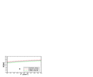
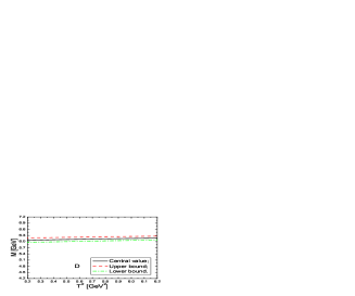
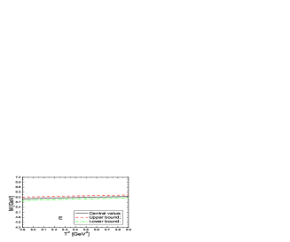
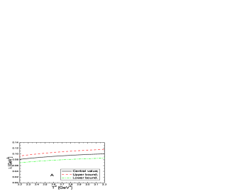
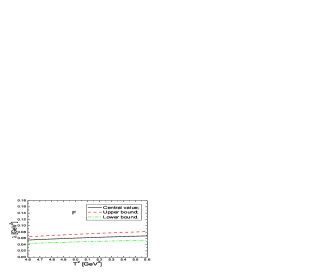
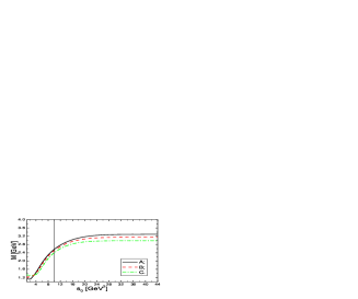
Taking into account all uncertainties of the parameters, we obtain the values of the masses and pole residues of the heavy baryon states, which are shown in Figs.1-2 and Table 2.

	$T^{2}(\rm{GeV}^{2})$	$\sqrt{s_{0}}(\rm{GeV})$	pole	perturbative
$\Omega_{b}$	$5.2-6.2$	$6.8$	$(45-60)\%$	$(83-88)\%$
$\Xi^{\prime}_{b}$	$4.9-5.9$	$6.7$	$(45-61)\%$	$(77-84)\%$
$\Sigma_{b}$	$4.6-5.6$	$6.6$	$(45-63)\%$	$(70-81)\%$
$\Omega_{c}$	$2.2-3.2$	$3.4$	$(46-75)\%$	$(75-86)\%$
$\Xi^{\prime}_{c}$	$2.0-3.0$	$3.3$	$(47-78)\%$	$(67-83)\%$
$\Sigma_{c}$	$1.8-2.8$	$3.2$	$(47-82)\%$	$(57-79)\%$

Table 1: The Borel parameters $T^{2}$ and threshold parameters $s_{0}$ for the heavy baryon states, the ”pole” stands for the contribution from the pole term, and the ”perturbative” stands for the contribution from the perturbative term in the operator product expansion.

	$T^{2}(\rm{GeV}^{2})$	$\sqrt{s_{0}}(\rm{GeV})$	$M(\rm{GeV})$	$\lambda(\rm{GeV}^{3})$	$M(\rm{GeV})[\rm{exp}]$
$\Omega_{b}$	$5.2-6.2$	$6.8\pm 0.1$	$6.11\pm 0.16$	$0.134\pm 0.030$	$6.165\cite[cite]{[\@@bibref{}{OmegabD0}{}{}]}/6.0544\cite[cite]{[\@@bibref{}{OmegabCDF}{}{}]}$
$\Xi^{\prime}_{b}$	$4.9-5.9$	$6.7\pm 0.1$	$5.96\pm 0.17$	$0.079\pm 0.020$	?
$\Sigma_{b}$	$4.6-5.6$	$6.6\pm 0.1$	$5.80\pm 0.19$	$0.062\pm 0.018$	5.8078($\Sigma_{b}^{+}$)/5.8152($\Sigma_{b}^{-}$) [1]
$\Omega_{c}$	$2.2-3.2$	$3.4\pm 0.1$	$2.70\pm 0.20$	$0.093\pm 0.023$	$2.6952$[1]
$\Xi^{\prime}_{c}$	$2.0-3.0$	$3.3\pm 0.1$	$2.56\pm 0.22$	$0.055\pm 0.016$	2.5756($\Xi^{{}^{\prime}+}_{c}$)/2.5779($\Xi^{{}^{\prime}0}_{c}$)[1]
$\Sigma_{c}$	$1.8-2.8$	$3.2\pm 0.1$	$2.40\pm 0.26$	$0.045\pm 0.015$	2.454[1]

Table 2: The masses $M(\rm{GeV})$ and pole residues $\lambda(\rm{GeV}^{3})$ of the heavy baryon states.

Figure 1: The masses $M$ of the heavy baryon states, the $A$, $B$, $C$, $D$, $E$ and $F$ correspond to the channels $\Omega_{c}$, $\Xi^{\prime}_{c}$, $\Sigma_{c}$, $\Omega_{b}$, $\Xi^{\prime}_{b}$ and $\Sigma_{b}$ respectively.

Figure 2: The pole residues $\lambda$ of the heavy baryon states, the $A$, $B$, $C$, $D$, $E$ and $F$ correspond to the channels $\Omega_{c}$, $\Xi^{\prime}_{c}$, $\Sigma_{c}$, $\Omega_{b}$, $\Xi^{\prime}_{b}$ and $\Sigma_{b}$ respectively.

Figure 3: The predicted masses with variation of the threshold parameters $s_{0}$, where the Borel parameters are taken to be the central values presented in Table 2, the $A$, $B$, $C$, $D$, $E$ and $F$ correspond to the channels $\Omega_{c}$, $\Xi^{\prime}_{c}$, $\Sigma_{c}$, $\Omega_{b}$, $\Xi^{\prime}_{b}$ and $\Sigma_{b}$ respectively.

From Table 2, we can see that the present predictions for the masses of the heavy baryons are consistent with the experimental data, the energy gap among the central values of the present predictions is about $M_{\Omega_{b}}-M_{\Xi^{\prime}_{b}}\approx M_{\Xi^{\prime}_{b}}-M_{\Sigma_{b}}\approx M_{\Omega_{c}}-M_{\Xi^{\prime}_{c}}\approx M_{\Xi^{\prime}_{c}}-M_{\Sigma_{c}}\approx 0.15\,\rm{GeV}$, which is excellent. The central value $M_{\Omega_{b}}=6.11\,\rm{GeV}$ lies between the experimental data $6.165\,\rm{GeV}$ from the D0 collaboration [23] and $6.0544\,\rm{GeV}$ from the CDF collaboration [33]. More experimental data is still needed to confirm the present predictions.

In Fig.3, we plot the predicted masses with variation of the threshold parameters $s_{0}$. From the figure, we can see that the predicted masses increase almost linearly with the threshold parameters $s_{0}$ for $s_{0}\leq 10\,\rm{GeV}^{2}$ in the charm channels and $s_{0}\leq 45\,\rm{GeV}^{2}$ in the bottom channels respectively. The threshold parameters should be taken around the critical points which are shown by the vertical lines in Fig.3, the values we choose in Table 2 are reasonable.

4 Conclusion

In this article, we re-study the heavy baryon states $\Omega_{Q}$, $\Xi^{\prime}_{Q}$ and $\Sigma_{Q}$ with the QCD sum rules, after subtracting the contributions from the corresponding negative parity heavy baryon sates, the predicted masses are in good agreement with the experimental data.

Appendix

The spectral densities of the heavy baryon states $\Omega_{Q}$, $\Xi^{\prime}_{Q}$ and $\Sigma_{Q}$ at the level of quark-gluon degrees of freedom,

$$\rho^{A}_{\Omega_{Q}}(p_{0}) = \frac{p_{0}}{16\pi^{4}}\int_{t_{i}}^{1}dtt(1-t)^{3}(p_{0}^{2}-\widetilde{m}_{Q}^{2})(5p_{0}^{2}-3\widetilde{m}_{Q}^{2})-\frac{p_{0}m_{s}\langle\bar{s}s\rangle}{\pi^{2}}\int_{t_{i}}^{1}dtt$$ (14)

$$+\frac{m_{s}\langle\bar{s}s\rangle}{\pi^{2}}\int_{t_{i}}^{1}dtt(1-t)\left[3p_{0}+\frac{\widetilde{m}_{Q}^{2}}{2}\delta(p_{0}-\widetilde{m}_{Q})\right]$$

$$-\frac{m_{s}\langle\bar{s}g_{s}\sigma Gs\rangle}{6\pi^{2}}\int_{0}^{1}dtt\left[1+\frac{\widetilde{m}_{Q}}{4T}\right]\delta(p_{0}-\widetilde{m}_{Q})$$

$$+\frac{m_{s}\langle\bar{s}g_{s}\sigma Gs\rangle}{8\pi^{2}}\delta(p_{0}-m_{Q})+\frac{\langle\bar{s}s\rangle^{2}}{3}\delta(p_{0}-m_{Q})$$

$$+\frac{p_{0}}{48\pi^{2}}\langle\frac{\alpha_{s}GG}{\pi}\rangle\int_{t_{i}}^{1}dt(4-5t)$$

$$+\frac{1}{96\pi^{2}}\langle\frac{\alpha_{s}GG}{\pi}\rangle\int_{t_{i}}^{1}dt(1-t)\widetilde{m}_{Q}^{2}\delta(p_{0}-\widetilde{m}_{Q})$$

$$-\frac{m_{Q}^{2}}{144\pi^{2}}\langle\frac{\alpha_{s}GG}{\pi}\rangle\int_{0}^{1}dt\frac{(1-t)^{3}}{t^{2}}\left[1+\frac{p_{0}}{4T}\right]\delta(p_{0}-\widetilde{m}_{Q})\,,$$

$$\rho^{B}_{\Omega_{Q}}(p_{0}) = \frac{3m_{Q}}{32\pi^{4}}\int_{t_{i}}^{1}dt(1-t)^{2}(p_{0}^{2}-\widetilde{m}_{Q}^{2})^{2}-\frac{3m_{s}m_{Q}\langle\bar{s}s\rangle}{2\pi^{2}}\int_{t_{i}}^{1}dt$$ (15)

$$+\frac{5m_{s}\langle\bar{s}g_{s}\sigma Gs\rangle}{24\pi^{2}}\delta(p_{0}-m_{Q})+\frac{2\langle\bar{s}s\rangle^{2}}{3}\delta(p_{0}-m_{Q})$$

$$+\frac{m_{Q}}{96\pi^{2}}\langle\frac{\alpha_{s}GG}{\pi}\rangle\int_{t_{i}}^{1}dt\left[-3-2t+\frac{2}{t^{2}}\right]$$

$$-\frac{m_{Q}}{192\pi^{2}}\langle\frac{\alpha_{s}GG}{\pi}\rangle\int_{0}^{1}dt\frac{(1-t)^{2}}{t}\widetilde{m}_{Q}\delta(p_{0}-\widetilde{m}_{Q})\,,$$

$$\rho^{A}_{\Xi^{\prime}_{Q}}(p_{0}) = \frac{p_{0}}{32\pi^{4}}\int_{t_{i}}^{1}dtt(1-t)^{3}(p_{0}^{2}-\widetilde{m}_{Q}^{2})(5p_{0}^{2}-3\widetilde{m}_{Q}^{2})-\frac{p_{0}m_{s}\langle\bar{q}q\rangle}{4\pi^{2}}\int_{t_{i}}^{1}dtt$$ (16)

$$+\frac{m_{s}\langle\bar{s}s\rangle}{4\pi^{2}}\int_{t_{i}}^{1}dtt(1-t)\left[3p_{0}+\frac{\widetilde{m}_{Q}^{2}}{2}\delta(p_{0}-\widetilde{m}_{Q})\right]$$

$$-\frac{m_{s}\langle\bar{s}g_{s}\sigma Gs\rangle}{24\pi^{2}}\int_{0}^{1}dtt\left[1+\frac{\widetilde{m}_{Q}}{4T}\right]\delta(p_{0}-\widetilde{m}_{Q})$$

$$+\frac{m_{s}\langle\bar{q}g_{s}\sigma Gq\rangle}{32\pi^{2}}\delta(p_{0}-m_{Q})+\frac{\langle\bar{q}q\rangle\langle\bar{s}s\rangle}{6}\delta(p_{0}-m_{Q})$$

$$+\frac{p_{0}}{96\pi^{2}}\langle\frac{\alpha_{s}GG}{\pi}\rangle\int_{t_{i}}^{1}dt(4-5t)$$

$$+\frac{1}{192\pi^{2}}\langle\frac{\alpha_{s}GG}{\pi}\rangle\int_{t_{i}}^{1}dt(1-t)\widetilde{m}_{Q}^{2}\delta(p_{0}-\widetilde{m}_{Q})$$

$$-\frac{m_{Q}^{2}}{288\pi^{2}}\langle\frac{\alpha_{s}GG}{\pi}\rangle\int_{0}^{1}dt\frac{(1-t)^{3}}{t^{2}}\left[1+\frac{\widetilde{m}_{Q}}{4T}\right]\delta(p_{0}-\widetilde{m}_{Q})\,,$$

$$\rho^{B}_{\Xi^{\prime}_{Q}}(p_{0}) = \frac{3m_{Q}}{64\pi^{4}}\int_{t_{i}}^{1}dt(1-t)^{2}(p_{0}^{2}-\widetilde{m}_{Q}^{2})^{2}-\frac{m_{s}m_{Q}\langle\bar{q}q\rangle}{2\pi^{2}}\int_{t_{i}}^{1}dt+\frac{m_{s}m_{Q}\langle\bar{s}s\rangle}{8\pi^{2}}\int_{t_{i}}^{1}dt$$ (17)

$$+\frac{m_{s}\left[6\langle\bar{q}g_{s}\sigma Gq\rangle-\langle\bar{s}g_{s}\sigma Gs\rangle\right]}{96\pi^{2}}\delta(p_{0}-m_{Q})+\frac{\langle\bar{q}q\rangle\langle\bar{s}s\rangle}{3}\delta(p_{0}-m_{Q})$$

$$+\frac{m_{Q}}{192\pi^{2}}\langle\frac{\alpha_{s}GG}{\pi}\rangle\int_{t_{i}}^{1}dt\left[-3-2t+\frac{2}{t^{2}}\right]$$

$$-\frac{m_{Q}}{384\pi^{2}}\langle\frac{\alpha_{s}GG}{\pi}\rangle\int_{0}^{1}dt\frac{(1-t)^{2}}{t}\widetilde{m}_{Q}\delta(p_{0}-\widetilde{m}_{Q})\,,$$

$$\rho^{A}_{\Sigma_{Q}}(p_{0}) = \frac{p_{0}}{32\pi^{4}}\int_{t_{i}}^{1}dtt(1-t)^{3}(p_{0}^{2}-\widetilde{m}_{Q}^{2})(5p_{0}^{2}-3\widetilde{m}_{Q}^{2})+\frac{\langle\bar{q}q\rangle^{2}}{6}\delta(p_{0}-m_{Q})$$ (18)

$$+\frac{p_{0}}{96\pi^{2}}\langle\frac{\alpha_{s}GG}{\pi}\rangle\int_{t_{i}}^{1}dt(4-5t)$$

$$+\frac{1}{192\pi^{2}}\langle\frac{\alpha_{s}GG}{\pi}\rangle\int_{t_{i}}^{1}dt(1-t)\widetilde{m}_{Q}^{2}\delta(p_{0}-\widetilde{m}_{Q})$$

$$-\frac{m_{Q}^{2}}{288\pi^{2}}\langle\frac{\alpha_{s}GG}{\pi}\rangle\int_{0}^{1}dt\frac{(1-t)^{3}}{t^{2}}\left[1+\frac{\widetilde{m}_{Q}}{4T}\right]\delta(p_{0}-\widetilde{m}_{Q})\,,$$

$$\rho^{B}_{\Sigma_{Q}}(p_{0}) = \frac{3m_{Q}}{64\pi^{4}}\int_{t_{i}}^{1}dt(1-t)^{2}(p_{0}^{2}-\widetilde{m}_{Q}^{2})^{2}+\frac{\langle\bar{q}q\rangle^{2}}{3}\delta(p_{0}-m_{Q})$$ (19)

$$+\frac{m_{Q}}{192\pi^{2}}\langle\frac{\alpha_{s}GG}{\pi}\rangle\int_{t_{i}}^{1}dt\left[-3-2t+\frac{2}{t^{2}}\right]$$

$$-\frac{m_{Q}}{384\pi^{2}}\langle\frac{\alpha_{s}GG}{\pi}\rangle\int_{0}^{1}dt\frac{(1-t)^{2}}{t}\widetilde{m}_{Q}\delta(p_{0}-\widetilde{m}_{Q})\,,$$

where $\widetilde{m}_{Q}^{2}=\frac{m_{Q}^{2}}{t}$, $t_{i}=\frac{m_{Q}^{2}}{p_{0}^{2}}$.

References

• [1] C. Amsler et al, Phys. Lett. B667 (2008) 1.
• [2] M. A. Shifman, A. I. Vainshtein and V. I. Zakharov, Nucl. Phys. B147 (1979) 385, 448.
• [3] L. J. Reinders, H. Rubinstein and S. Yazaki, Phys. Rept. 127 (1985) 1.
• [4] E. Bagan, M. Chabab, H. G. Dosch, and S. Narison, Phys. Lett. B278, 367 (1992).
• [5] E. Bagan, M. Chabab, H. G. Dosch, and S. Narison, Phys. Lett. B287, 176 (1992).
• [6] Z. G. Wang, Eur. Phys. J. C54 (2008) 231.
• [7] F. O. Duraes and M. Nielsen, Phys. Lett. B658 (2007) 40.
• [8] J. R. Zhang and M. Q. Huang, Phys. Rev. D77 (2008) 094002.
• [9] J. R. Zhang and M. Q. Huang, Phys. Rev. D78 (2008) 094015.
• [10] M. Albuquerque, S. Narison and M. Nielsen, arXiv:0904.3717.
• [11] Z. G. Wang, Eur. Phys. J. C61 (2009) 321.
• [12] Z. G. Wang, arXiv:0910.2112.
• [13] E. V. Shuryak, Nucl. Phys. B198, 83 (1982).
• [14] A. G. Grozin and O. I. Yakovlev, Phys. Lett. B285, 254 (1992).
• [15] E. Bagan, M. Chabab, H. G. Dosch and S. Narison, Phys. Lett. B301, 243 (1993).
• [16] Y. B. Dai, C. S. Huang, C. Liu and C. D. Lu, Phys. Lett. B371, 99 (1996).
• [17] Y. B. Dai, C. S. Huang, M. Q. Huang and C. Liu, Phys. Lett. B387, 379 (1996).
• [18] D. W. Wang, M. Q. Huang and C. Z. Li, Phys. Rev. D65, 094036 (2002).
• [19] S. L. Zhu, Phys. Rev. D61, 114019 (2000).
• [20] C. S. Huang, A. L. Zhang and S. L. Zhu, Phys. Lett. B492, 288 (2000).
• [21] D. W. Wang and M. Q. Huang, Phys. Rev. D68, 034019 (2003).
• [22] X. Liu, H. X. Chen, Y. R. Liu, A. Hosaka, and S. L. Zhu, Phys. Rev. D77, 014031 (2008).
• [23] V. Abazov et al, Phys. Rev. Lett. 101 (2008) 232002.
• [24] R. Roncaglia, D. B. Lichtenberg, and E. Predazzi, Phys. Rev. D52, 1722 (1995).
• [25] A. Valcarce, H. Garcilazo, J. Vijande, Eur. Phys. J. A37 (2008) 217.
• [26] E. Jenkins, Phys. Rev. D54, 4515 (1996).
• [27] K. C. Bowler et al., Phys. Rev. D54, 3619 (1996).
• [28] N. Mathur, R. Lewis, and R. M. Woloshyn, Phys. Rev. D66, 014502 (2002).
• [29] D. Ebert, R. N. Faustov, and V. O. Galkin, Phys. Rev. D72, 034026 (2005).
• [30] D. Ebert, R. N. Faustov, and V. O. Galkin, Phys. Lett. B659, 612 (2008).
• [31] M. Karliner, B. Keren-Zura, H. J. Lipkin, and J. L.Rosner, arXiv:0706.2163; arXiv:0708.4027.
• [32] W. Roberts and M. Pervin, Int. J. Mod. Phys. A23 (2008) 2817.
• [33] T. Aaltonen et al, Phys. Rev. D80 (2009) 072003.
• [34] L. Liu, H. W. Lin, K. Orginos and A. Walker-Loud, arXiv:0909.3294.
• [35] D. Jido, N. Kodama and M. Oka, Phys. Rev. D54 (1996) 4532.
• [36] Y. Chung, H. G. Dosch, M. Kremer and D. Schall, Nucl. Phys. B197 (1982) 55.
• [37] Z. G. Wang, arXiv:0909.4144.
• [38] R. L. Jaffe and F. Wilczek, Phys. Rev. Lett. 91 (2003) 232003.
• [39] R. L. Jaffe, Phys. Rept. 409 (2005) 1.
• [40] B. L. Ioffe, Prog. Part. Nucl. Phys. 56 (2006) 232.
• [41] P. Colangelo and A. Khodjamirian, hep-ph/0010175.
• [42] S. Narison, Camb. Monogr. Part. Phys. Nucl. Phys. Cosmol. 17 (2002) 1.
• [43] A. Khodjamirian and R. Ruckl, Adv. Ser. Direct. High Energy Phys. 15 (1998) 345.