The GALEX Arecibo SDSS Survey. I. Gas Fraction Scaling Relations of Massive Galaxies and First Data Release

Abstract

We introduce the GALEX Arecibo SDSS Survey (GASS), an on-going large program that is gathering high quality Hi-line spectra using the Arecibo radio telescope for an unbiased sample of $\sim$1000 galaxies with stellar masses greater than $10^{10}$ M_⊙ and redshifts $0.025<z<0.05$, selected from the SDSS spectroscopic and GALEX imaging surveys. The galaxies are observed until detected or until a low gas mass fraction limit (1.5$-$5%) is reached. This paper presents the first Data Release, DR1, consisting of $\sim$20% of the final GASS sample. We use this data set to explore the main scaling relations of Hi gas fraction with galaxy structure and NUV-r colour. A large fraction ($\sim$60%) of the galaxies in our sample are detected in Hi. Even at stellar masses above $10^{11}$ M_⊙, the detected fraction does not fall below $\sim$40%. We find that the atomic gas fraction $M_{\rm HI}$/$M_{\star}$ decreases strongly with stellar mass, stellar surface mass density and NUV$-r$ colour, but is only weakly correlated with galaxy bulge-to-disk ratio (as measured by the concentration index of the r-band light). We also find that the fraction of galaxies with significant (more than a few percent) Hi decreases sharply above a characteristic stellar surface mass density of $10^{8.5}$ M_⊙ kpc^-2. The fraction of gas-rich galaxies decreases much more smoothly with stellar mass. One of the key goals of the GASS survey is to identify and quantify the incidence of galaxies that are transitioning between the blue, star-forming cloud and the red sequence of passively-evolving galaxies. Likely transition candidates can be identified as outliers from the mean scaling relations between $M_{\rm HI}$/$M_{\star}$ and other galaxy properties. We have fit a plane to the 2-dimensional relation between Hi mass fraction, stellar surface mass density, and NUV$-r$ colour. Interesting outliers from this plane include gas-rich red sequence galaxies that may be in the process of regrowing their disks, as well as blue, but gas-poor spirals.

1 Introduction

There are good reasons to investigate how and why the cold gas content of a massive galaxy varies with stellar mass and other physical properties relating to its growth history. While the distinction between red, old ellipticals and blue, star-forming spirals has been known for a long time, recent work based on the Sloan Digital Sky Survey (SDSS; York et al., 2000) has shown that galaxies appear to divide into two distinct “families” at a stellar mass $M_{\star}$$\sim$3 $\times$$10^{10}$ M_⊙ (Strateva et al., 2001; Kauffmann et al., 2003; Baldry et al., 2004). Lower mass galaxies typically have young stellar populations, low surface mass densities and the low concentrations characteristic of disks. On the other hand, galaxies with old stellar populations, high surface mass densities and the high concentrations typical of bulges tend to have higher mass. New theoretical work has led to a diverse set of possible mechanisms to explain this characteristic mass scale where galaxies transition from young to old (Kereš et al., 2005; Dekel & Birnboim, 2006; Hopkins et al., 2008), with nearly all operating via quenching or regulation of the gas supply (e.g., Martin et al., 2007). Observations of the cold Hi gas component – the source of the material that will eventually form stars – in galaxies across the transition mass, will provide an important new test of those models.

Initial clues can come from the study of the Hi scaling relations of massive galaxies. Early seminal work (e.g., Haynes & Giovanelli 1984; Knapp, Turner, & Cunniffe 1985; Roberts et al. 1991; see Roberts & Haynes 1994 for a review) took the first step towards answering the question of how the Hi properties of galaxies vary as a function of morphological type, environment and other physical properties. Although massive “transition” galaxies are found in these and more recent samples (Paturel et al. 2003; Springob et al. 2005, hereafter S05; Bothwell, Kennicutt & Lee 2009), the selection criteria make it difficult to identify these in a robust way. One needs to quantify the distribution of gas fraction as a function of $M_{\star}$, colour, star formation rate (SFR) and other galaxy properties in order to understand which galaxies are more gas rich or gas poor than the mean.

It has become common practice to use “photometric gas-fractions” (Bell et al., 2003; Kannappan, 2004; Zhang et al., 2009), which exploit the well-known connection between SFR and gas content (Schmidt, 1959; Kennicutt, 1998), as a substitute for real gas measurements. However, these derived average relations cannot be used to study if and how the gas content relates to other properties and physical conditions in the galaxies.

Hi studies of transition objects require large and uniform samples spanning a wide range in gas fraction, stellar mass and other galaxy properties (e.g., structural parameters and star formation). Although blind surveys offer the required uniformity, Hi studies of transition galaxies are currently not possible because the depths reached by existing wide-area blind Hi surveys are very shallow compared to surveys such as the SDSS. The Hi Parkes All-Sky Survey (Barnes et al., 2001; Meyer et al., 2004), covered $\sim 30000$ deg² and produced a final catalog of around 5000 Hi detections with a median redshift of 2800 km s^-1. This should be contrasted with the main SDSS spectroscopic survey, which covers around 7000 deg² and contains more than half a million galaxies with a median redshift of 30,000 km s^-1. The recently initiated Arecibo Legacy Fast ALFA survey (ALFALFA; Giovanelli et al., 2005) is mapping 7000 deg² to considerably deeper limits. With a median redshift of $\sim$9100 km s^-1, ALFALFA for the first time samples the Hi population over a cosmologically fair volume, and is expected to detect $\sim$30,000 extragalactic Hi-line sources out to redshifts of $z\sim 0.06$. Even so, the galaxies in the transition regime detected with ALFALFA will be predominantly gas-rich.

In this paper we describe the first results and data release from the GALEX Arecibo SDSS Survey (GASS), a new Hi survey specifically designed to obtain Hi measurements of $\sim$1000 galaxies in the local universe ($0.025<z<0.05$) with stellar masses $M_{\star}>10^{10}$ M_⊙. As we discuss below, we observe these massive galaxies down to a low gas mass fraction limit (1.5$-$5%), in order to study the physical mechanisms that shape the stellar mass function, regulate gas accretion and quench further galaxy growth by conversion of gas into stars. We expect that GASS will provide a rich, homogeneous data set of structural and physical parameters (e.g., luminosity, stellar mass, size, surface brightness, gas-phase and stellar metallicities, AGN content, velocity dispersion), star formation rates and gas properties. Analysis of this unique sample should allow us, for the first time, to investigate how the cold gas responds to a variety of different physical conditions in the galaxy and obtain new insights on the physical processes responsible for the transition between blue, star-forming spirals and red, passively-evolving ellipticals.

In a companion paper (Schiminovich et al., in preparation; hereafter Paper II), we derive volume-averaged quantities for our GASS sample to determine the relative fraction of Hi associated with massive galaxies in the local universe, and compare with the SFR density to explore how the gas consumption timescale varies across the galaxy population. In both papers we also discuss how we expect to refine and improve our analyses using the full GASS data set.

In this first paper we describe GASS survey design and selection criteria (§ 2 and § 3). Arecibo observations and data processing are discussed in § 4. We provide catalogs of SDSS/GALEX parameters and Hi-line spectroscopy measurements for the 176 galaxies in this first Data Release (DR1) in § 5 and § 6, respectively. Our results are presented in § 7. We characterize the properties of the DR1 data set in § 7.1. In order to obtain a sample that is unbiased in terms of Hi properties, we need to correct for the fact that we do not re-observe objects already detected by ALFALFA or galaxies found in the Cornell Hi archive (S05). We construct such a representative sample in § 7.2, and we use it to quantify average gas fraction scaling relations as a function of other galaxy parameters in § 7.3 and § 7.4. Our findings are summarized and further discussed in § 8.

All the distance-dependent quantities in this work are computed assuming $\Omega=0.3$, $\Lambda=0.7$ and $H_{0}=70$ km s^-1 Mpc^-1. AB magnitudes are used throughout the paper.

2 Survey Design

GASS is designed to efficiently measure the Hi content of an unbiased sample of $\sim$1000 massive galaxies, for which SDSS spectroscopy and GALEX (Martin et al., 2005) imaging are also available. As described below, the targets are selected only by redshift and stellar mass, and observed with the Arecibo radio telescope until detected or until a gas fraction limit of $1.5-5$% is reached (i.e., a gas fraction limit an order of magnitude lower than in objects of similar stellar mass detected by ALFALFA at the same redshifts). We describe below our survey requirements and sample selection methodology.

Survey footprint. All the GASS targets are located within the intersection of the footprints of the SDSS primary spectroscopic survey, the projected GALEX Medium Imaging Survey (MIS) and ALFALFA. The SDSS primary spectroscopic sample targets all galaxies with $r<17.77$ with high completeness ($>80$% for $r>14.5$). The GALEX MIS reaches limiting NUV magnitude $\sim$23, which allows us to probe the full range of colours (and derived SFRs) of the normal galaxy population. Existing ALFALFA coverage increases our survey efficiency by allowing us to remove from the GASS target list any objects already detected by ALFALFA — this amounts to an estimated 20% of the galaxies meeting our selection criteria. However, this does not correspond to a 20% gain in observing time, because the objects that we skip are those that would be detected with the shortest integrations. We also do not re-observe galaxies with detections in the Cornell Hi digital archive of targeted observations (S05), a homogeneous compilation of Hi parameters for $\sim$9000 optically-selected galaxies, mostly selected for Tully-Fisher applications.

Stellar mass range ($10<{\rm Log}M_{\star}/M_{\odot}<11.5$). We target a stellar mass range that straddles the “transition mass” at $\sim$$3\times 10^{10}$ M_⊙.

Redshift range ($0.025<z<0.05$). An Hi survey of massive galaxies selected from SDSS is ideally performed at redshifts above $z>0.025$. At magnitudes brighter than $r\sim 13$ (corresponding to a transition mass galaxy at $z=0.025$), the spectroscopic targeting completeness in the SDSS falls below 50%. Additionally, a single pointing on galaxies at $z<0.025$ may occasionally underestimate the Hi flux, if their Hi disks are extended in comparison with the Arecibo beam. The upper end of our redshift interval is set by practical sensitivity limits as well as a desire to remain within the velocity range covered by ALFALFA ($0<z<0.06$). We further restricted the range to $z<0.05$ in order to avoid the gap in ALFALFA velocity coverage caused by radio frequency interference (RFI) at 1350 MHz from the the Federal Aviation Administration (FAA) radar in San Juan.

Gas mass fraction/gas mass limit. A crucial goal of GASS is to identify galaxies that show signs of recent accretion and/or quenching. We wish to obtain accurate gas mass measurements for transition galaxies, which have had a small, but significant amount of recent star formation ($1-5$% of their total mass). This translates into a requirement that we observe the sample to an equivalent gas mass fraction (defined as $M_{\rm HI}$/$M_{\star}$ in this work) limit. Practically, we have set a limit of $M_{\rm HI}/M_{\star}>0.015$ for galaxies with $M_{\star}$$>10^{10.5}$ M_⊙, and a constant gas mass limit $M_{\rm HI}$$=10^{8.7}$ M_⊙ for galaxies with smaller stellar masses. This corresponds to a gas fraction limit $0.015-0.05$ for the whole sample. This allows us to detect galaxies with gas fractions significantly below those of the Hi-rich ALFALFA detections at the same redshifts, and find early-type transition galaxies harboring significant reservoirs of gas. We do not try to detect inconsequential amounts of gas ($M_{\rm HI}/M_{\star}<0.01$) typical of the most gas-poor early-types.

Based on the Hi mass limit assigned to each galaxy (i.e., $M_{\rm HI}$$=10^{8.7}$ M_⊙ or 0.015 $M_{\star}$, whichever is larger), we have computed the observing time, $T_{\rm max}$, required to reach that value with our observing mode and instrumental setup (see § 5).

3 Sample Selection

Since the ALFALFA and GALEX surveys are on-going, we have defined a GASS parent sample, based on SDSS DR6 (Adelman-McCarthy et al., 2008) and the maximal ALFALFA footprint, from which the targets for Arecibo observations are extracted. The parent sample includes 12006 galaxies that satisfy our stellar mass and redshift selection criteria (see Fig. 1); of these, $\sim$10000 have UV photometry from either the GALEX All-sky Imaging Survey (AIS; $\sim$100 s exposure, FUV_lim, NUV${}_{lim}<21~{}m_{\rm AB}$) or the MIS ($\sim$1500 s exposure, FUV_lim, NUV${}_{lim}<23~{}m_{\rm AB}$). The final GASS sample will include $\sim$1000 galaxies, chosen by randomly selecting a subset which balances the distribution across stellar mass and which maximizes existing GALEX exposure time. In practice, we have extracted a subset of few hundred targets distributed across the whole GASS footprint, which includes galaxies that already have MIS or at least AIS data, and we have given highest priority to those in the sky regions already catalogued by ALFALFA. We have also given some priority to objects with stellar mass greater than 10^10.5 M_⊙, but the final survey sample will have similar numbers of galaxies in each stellar mass bin.

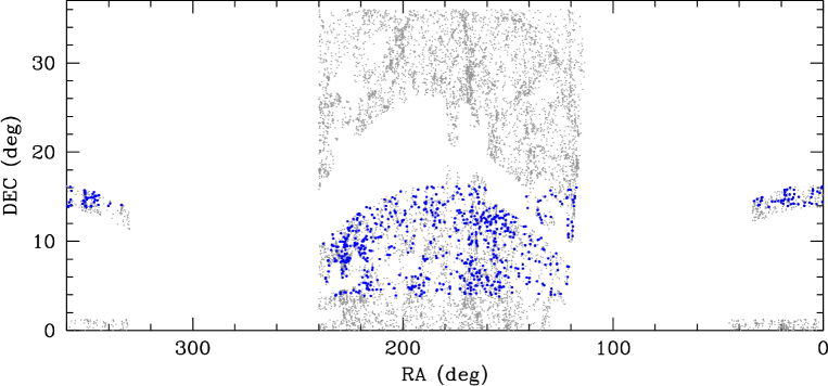
Figure 1: Sky footprint of the GASS survey. Gray points represent galaxies in the parent sample, the super-set of $\sim$12000 objects out of which targets for Arecibo observations are extracted. Blue points indicate the subset of galaxies detected by the ALFALFA survey to date.

3.1 Overlap with ALFALFA and Cornell Digital Hi archive

As mentioned in § 2, we do not re-observe galaxies with good Hi measurements already available from either ALFALFA or the S05 digital archive. The overlap between the GASS parent sample and the S05 compilation of detected galaxies (their Table 3) is 430 objects. ALFALFA has released five catalogs to date, three of which are in sky regions with SDSS spectroscopic coverage (Giovanelli et al., 2007; Kent et al., 2008; Stierwalt et al., 2009). Together with still unpublished data, ALFALFA has fully catalogued the following two sky regions relevant for GASS: (a) $7.5<\alpha_{2000}<16.5$ hrs, $+4^{\circ}<\delta_{2000}<+16^{\circ}$, and (b) $22<\alpha_{2000}<3$ hrs, $+14^{\circ}<\delta_{2000}<+16^{\circ}$. Notice that the only ALFALFA detections that we do not re-observe are the ones classified as reliable (i.e., “code 1” in their tables); we do target the ALFALFA priors, i.e. candidate sources with lower signal-to-noise ($<6.5$) but optical counterparts with known and matching redshift (“code 2”). These sources are usually confirmed by GASS observations and detected with short integrations (13 of the 176 DR1 galaxies are classified as ALFALFA code 2. They were all detected except one). In the rest of this paper, “ALFALFA detections” will refer only to the galaxies in the first category. Figure 1 shows the sky distribution of the 769 sources meeting GASS selection criteria that have been detected by the ALFALFA survey to date (blue points). These are divided into 658 in the region (a) defined above and 81 in (b), corresponding to 18% and 19% of the parent sample in the same areas. The S05 archive contributes 195 galaxies to region (a) and 45 to (b), the large majority of which are also ALFALFA detections (but the S05 Hi profiles have higher signal-to noise). After removing duplicates, the numbers of available Hi detections in regions (a) and (b) are 710 and 89, respectively.

4 Arecibo Observations and Data Reduction

GASS observations started in March 2008 and are on-going. In the first 1.5 years of the survey until end of August 2009, Arecibo allocated 239 hours to this project, with approximately 40 hours lost to technical or RFI problems. The observations were scheduled in 85 blocks of 1$-$6.25 hours, with about 50% of the total allocation time in blocks of 3 hours or less. The full survey will require a total of $\sim$900 hours to be completed (not including the increased overhead caused by the scheduling in short blocks). Most of the observing ($\sim$160 hours) has been carried out remotely from the MPA in Garching. Since May 2009, remote observations are also done from Columbia, JHU, and NYU.

The Hi observations are done in standard position-switching mode: each observation consists of an on/off source pair, each typically integrated for 5 minutes, followed by the firing of a calibration noise diode. We use the L-band wide receiver, which operates in the frequency range 1120$-$1730 MHz, with a 1280$-$1470 MHz filter to limit the impact of RFI on our observations. The interim correlator is used as a backend. The spectra are recorded every second with 9-level sampling. Two correlator boards, each configured for 12.5 MHz bandwidth, one polarization, and 2048 channels per spectrum (yielding a velocity resolution of 1.4 km s^-1 at 1370 MHz before smoothing) are centered at or near the frequency corresponding to the SDSS redshift of the target. The other two boards are configured for 25 MHz bandwidth, two polarizations, 1024 channels per spectrum, and are centered at 1365 and 1385 MHz, respectively. This setup allows us to monitor the full frequency interval of the GASS targets (1353 to 1386 MHz, corresponding to $z=0.050$ and $z=0.025$, respectively) for RFI and other problems. All the observations are done during night-time to minimize the impact of RFI and solar standing waves on our data. The Doppler correction for the motion of the Earth is applied during off-line processing.

A radar blanker is used for $\sim$2/3 of our targets (those below 1375 MHz) to avoid RFI caused by harmonics of the FAA airport radar in San Juan, which transmits at 1330 and 1350 MHz. This device is synchronized with the pulsed signal of the radar — the data acquisition with the interim correlator is effectively interrupted for a time $\delta t$ during and after each radar pulse ($\delta t$ can be chosen by the observer to lie between 100 and 750 $\mu$s, and is typically set to 400 $\mu$s to block, in addition to the radar pulse, its delayed reflections from aircraft or other obstacles).

The target lists for the observing runs are prepared in advance. The selection is made from the compilation of galaxies mentioned in § 3, only a small subset of which are visible during each given observing window. The GASS targets are randomly chosen from that subset, after excluding galaxies with prior Hi detections from ALFALFA or the S05 archive, or with strong continuum sources within the beam that would cause ripples in the baselines.

We usually acquire up to three 5-minute on-off pairs per object per observing session, and accumulate observations from multiple sessions. One such pair requires approximately 13.5 or 11.3 minutes with or without the radar blanker, respectively, and exclusive of slew-to-source time. For galaxies with $T_{\rm max}\leq 4$ minutes, or to use end-of-run blocks of order of 10 minutes, we acquire 4-minute pairs instead, but not shorter. This is a good compromise between obtaining good quality profiles with small time investment for Hi-rich objects and minimizing overheads (which increase when an observation is broken into smaller time segments). On-source integration times for the sample presented in this work ranged between 4 and 90 minutes, with an average of 13 minutes for the detections and 23 minutes for the non-detections (total times are $\sim$2.5 times longer).

GASS spectra are quickly combined and processed during the observations in order to assess data quality, and to allow us to stop the integration when the object is detected, or when the maximum time to reach its limiting gas fraction has been reached. A more careful data reduction, which includes RFI excision, is performed off-line at a later stage.

The data reduction is performed in the IDL environment using our own routines, which are based on the standard Arecibo data processing library developed by Phil Perillat. More specifically, we adapted the software written to process and measure the observations described in Catinella et al. (2008), which, apart for targeting higher redshift objects, adopted identical observing mode and setup. In summary, the data reduction of each polarization and on-off pair includes Hanning smoothing, bandpass subtraction, RFI excision, and flux calibration. A total spectrum is obtained for each of the two orthogonal linear polarizations by combining good quality records (those without serious RFI or standing waves). Each pair is weighted by a factor $1/rms^{2}$, where $rms$ is the root mean square noise measured in the signal-free portion of the spectrum. The two polarizations are separately inspected (they usually agree well. If present, polarization mismatches are noted in the Appendix), and averaged to produce the final spectrum.

After boxcar smoothing and baseline subtraction, the Hi-line profiles are ready for the measurement of redshift, rotational velocity and integrated Hi line flux. Recessional and rotational velocities are measured at the 50% peak level from linear fits to the edges of the Hi profile. Our measurement technique is explained in more detail, e.g., in Catinella, Haynes, & Giovanelli (2007, §2.2).

5 SDSS and GALEX Data

This section summarizes the quantities derived from optical and UV data used in this paper. All the optical parameters listed below were obtained from Structured Query Language (SQL) queries to the SDSS DR7 database server, unless otherwise noted.

The GALEX UV photometry for our sample was completely reprocessed by us, as explained in Wang et al. (2009). Briefly, we registered GALEX NUV/FUV and SDSS r-band images, and convolved the latter to the (lower resolution) UV Point Spread Function (PSF) using Image Reduction and Analysis Facility (IRAF) tasks. The UV PSFs are measured from stacked stellar images, obtained by co-adding the stars within 1200 pixels from the center of the frame. After masking out nearby sources detected in either UV or convolved SDSS r-band images, we used SExtractor (Bertin & Arnouts, 1996) to calculate magnitudes within Kron elliptical apertures, defined on the convolved SDSS images.

The NUV$-r$ colours thus derived are corrected for Galactic extinction following Wyder et al. (2007), who adopted $A(\lambda)/E(B-V)=2.751$ for the SDSS r-band and $A(\lambda)/E(B-V)=8.2$ for GALEX NUV. From these assumptions, the correction to be applied to NUV$-r$ colours is $A_{NUV}-A_{r}=1.9807A_{r}$, where the extinction $A_{r}$ is obtained from the SDSS data base (listed in Table 1 below as “$ext_{r}$”).

Internal dust attenuation corrections are very uncertain for galaxies outside the blue sequence, especially in absence of far infrared data (e.g., Johnson et al., 2007; Wyder et al., 2007; Cortese et al., 2008). Moreover, obtaining reliable SFRs from NUV photometry is not trivial in the poorly calibrated, low specific SFR regime (e.g., Schiminovich et al., 2007; Salim et al., 2007). A detailed discussion of these issues is beyond the scope of this work, and is presented in Paper II. Hence, we do not correct NUV$-r$ colours for dust attenuation, nor we derive dust-corrected SFRs in this paper.

Table 1 lists the relevant SDSS and UV quantities for the GASS objects published in this work, ordered by increasing right ascension:
Cols. (1) and (2): GASS and SDSS identifiers.
Col. (3): SDSS redshift, $z_{\rm SDSS}$. The typical uncertainty of SDSS redshifts for this sample is 0.0002.
Col. (4): base-10 logarithm of the stellar mass, $M_{\star}$, in solar units. Stellar masses are derived from SDSS photometry using the methodology described in Salim et al. 2007 (a Chabrier 2003 initial mass function is assumed). Over our required stellar mass range, these values are believed to be accurate to better than 30%, significantly smaller than the uncertainty on other derived physical parameters such as star formation rates. This accuracy in $M_{\star}$ is more than sufficient for this study.
Col. (5): radius containing 50% of the Petrosian flux in z-band, $R_{50,z}$, in arcsec.
Cols. (6) and (7): radii containing 50% and 90% of the Petrosian flux in r-band, $R_{50}$ and $R_{90}$ respectively, in arcsec (for brevity, we omit the subscript “$r$” from these quantities throughout the paper).
Col. (8): base-10 logarithm of the stellar mass surface density, $\mu_{\star}$, in M_⊙ kpc^-2. This quantity is defined as $\mu_{\star}=M_{\star}/(2\pi R_{50,z}^{2})$, with $R_{50,z}$ in kpc units.
Col. (9): Galactic extinction in r-band, ext_r, in magnitudes, from SDSS.
Col. (10): r-band model magnitude from SDSS, $r$, corrected for Galactic extinction.
Col. (11): NUV$-r$ observed colour from our reprocessed photometry, corrected for Galactic extinction.
Col. (12): exposure time of GALEX NUV image, T_NUV, in seconds.
Col. (13): maximum on-source integration time, $T_{\rm max}$, required to reach the limiting Hi mass fraction, in minutes (see § 2). Given the Hi mass limit of the galaxy (set by its gas fraction limit and stellar mass), we computed the required integration time to reach this limit at the galaxy’s redshift, assuming a 5$\sigma$ signal with 300 km s^-1 velocity width and the instrumental parameters typical of our observations (i.e., gain $\sim$10 K Jy^-1 and system temperature $\sim$28 K at 1370 MHz).

6 Hi Source Catalogs

In this section we present the main Hi parameters of the 99 galaxies detected by GASS to date, and provide upper limits for the 77 objects that were not detected.

Table 2 lists the derived Hi quantities for the detected galaxies (ordered by increasing right ascension), namely:
Cols. (1) and (2): GASS and SDSS identifiers.
Col. (3): SDSS redshift, $z_{\rm SDSS}$, repeated here from Table 1 to facilitate the comparison with the Hi measurement (col. 6).
Col. (4): on-source integration time of the Arecibo observation, $T_{\rm on}$, in minutes. This number refers to on scans that were actually combined, and does not account for possible losses due to RFI excision (usually negligible).
Col. (5): velocity resolution of the final, smoothed spectrum in km s^-1.
Col. (6): redshift, $z$, measured from the Hi spectrum. The error on the corresponding heliocentric velocity, $cz$, is half the error on the width, tabulated in the following column.
Col. (7): observed velocity width of the source line profile in km s^-1, $W_{50}$, measured at the 50% level of each peak. The error on the width is the sum in quadrature of the statistical and systematic uncertainties in km s^-1. Statistical errors depend primarily on the signal-to-noise of the Hi spectrum, and are obtained from the rms noise of the linear fits to the edges of the Hi profile. Systematic errors depend on the subjective choice of the Hi signal boundaries, and are estimated as explained in Giovanelli et al. (2007). These are negligible for most of the galaxies in this sample (only 17 objects have systematic errors greater than zero).
Col. (8): velocity width corrected for instrumental broadening and cosmological redshift only, $W_{50}$^c, in km s^-1. No inclination or turbulent motion corrections are applied.
Col. (9): observed, integrated Hi-line flux density in Jy km s^-1, $F\equiv\int S~{}dv$, measured on the smoothed and baseline-subtracted spectrum. The reported uncertainty is the sum in quadrature of the statistical and systematic errors (see col. 7). The statistical errors are calculated according to equation 2 of S05.
Col. (10): rms noise of the observation in mJy, measured on the signal- and RFI-free portion of the smoothed spectrum.
Col. (11): signal-to-noise ratio of the Hi spectrum, S/N, estimated following Saintonge (2007) and adapted to the velocity resolution of the spectrum. This is the definition of S/N adopted by ALFALFA, which accounts for the fact that for the same peak flux a broader spectrum has more signal.
Col. (12): base-10 logarithm of the Hi mass, $M_{\rm HI}$, in solar units, computed via:

$$\frac{M_{\rm HI}}{\rm M_{\odot}}=\frac{2.356\times 10^{5}}{1+z}\left[\frac{d_{\rm L}(z)}{\rm Mpc}\right]^{2}\left(\frac{\int S~{}dv}{\rm Jy~{}km~{}s^{-1}}\right)$$ (1)

where $d_{\rm L}(z)$ is the luminosity distance to the galaxy at redshift $z$ as measured from the Hi spectrum.
Col. (13): base-10 logarithm of the Hi mass fraction, $M_{\rm HI}$/$M_{\star}$.
Col. (14): quality flag, Q (1=good, 2=marginal, 5=confused). An asterisk indicates the presence of a note for the source in the Appendix. Code 1 refers to reliable detections, with a S/N ratio of order of 6.5 or higher (this is the same threshold adopted by ALFALFA). Marginal detections have lower S/N, thus more uncertain Hi parameters, but are still secure detections, with Hi redshift consistent with the SDSS one. The S/N limit is not strict, but depends also on Hi profile and baseline quality. As a result, galaxies with S/N slightly above the threshold but with uncertain profile or bad baseline may be flagged with a code 2, and objects with S/N $\lesssim 6.5$ and Hi profile with well-defined edges may be classified as code 1. We assigned the quality flag 5 to four “confused” galaxies, where most of the Hi emission is believed to come from another source within the Arecibo beam. For some of the galaxies, the presence of small companions within the beam might contaminate (but is unlikely to dominate) the Hi signal – this is just noted in the Appendix. Finally, we assigned code 3 to GASS 9463, which is both marginal and confused.

Table 3 gives the derived Hi upper limits for the non-detections. Columns (1-4) and (5) are the same as columns (1-4) and (10) in Table 2, respectively. Column (6) lists the upper limit on the Hi mass in solar units, Log $M_{\rm HI}$_,lim, computed assuming a 5 $\sigma$ signal with 300 km s^-1 velocity width, if the spectrum was smoothed to 150 km s^-1. Column (7) gives the corresponding upper limit on the gas fraction, Log $M_{\rm HI}$_,lim/$M_{\star}$. An asterisk in Column (8) indicates the presence of a note for the galaxy in the Appendix.

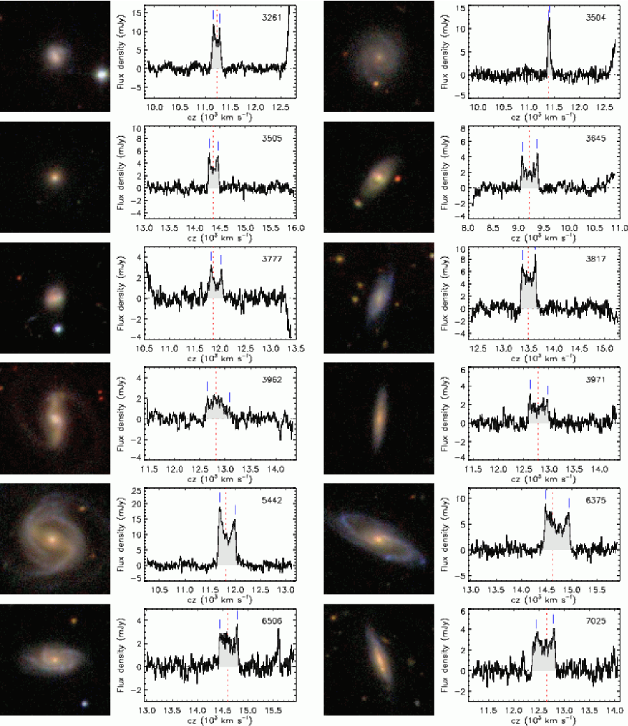
Figure 2: SDSS postage stamp images (1 arcmin square) and Hi-line profiles of the survey detections, ordered by increasing GASS number (indicated in each spectrum). The Hi spectra are calibrated, smoothed and baseline-subtracted. A dotted line and two dashes indicate the heliocentric velocity corresponding to the SDSS redshift and the two peaks used for width measurement, respectively. [See the electronic edition of the Journal for the complete figure.]

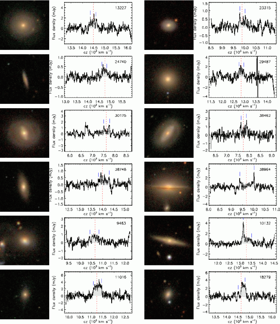
Figure 3: Same as Fig. 2 for marginal (first four rows) or confused (last two rows; GASS 9463 is both marginal and confused) detections. [See the electronic edition of the Journal for the complete figure.]

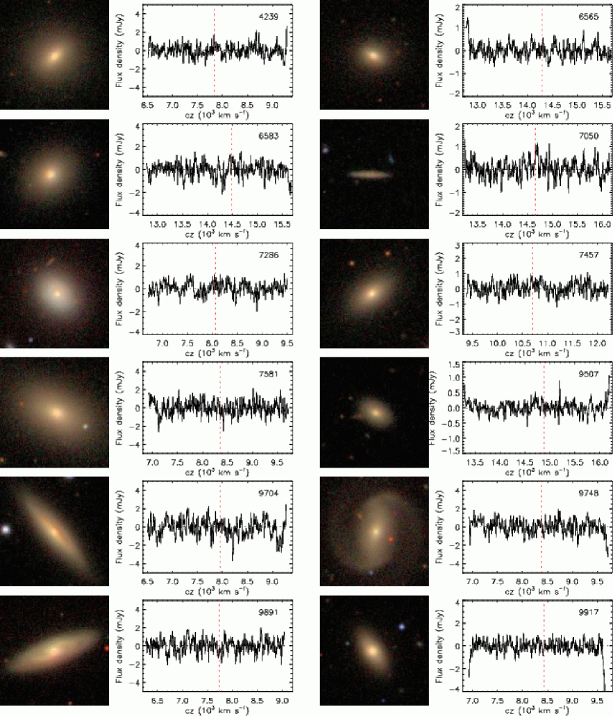
Figure 4: Same as Fig. 2 for non-detections. [See the electronic edition of the Journal for the complete figure.]

Figure 2 shows SDSS images and Hi spectra for the galaxies with quality flag 1 in Table 2; marginal detections and galaxies for which confusion is certain are shown separately in Figure 3, and non-detections are presented in Figure 4. The objects in these figures are ordered by increasing GASS number (indicated on the top right corner of each spectrum). The SDSS images show a 1 arcmin square field, i.e., only the central part of the region sampled by the Arecibo beam (the half power full width of the beam is $\sim$3.5′ at the frequencies of our observations). Therefore, companions that might be detected in our spectra typically are not visible in the postage stamps – examples include GASS 40007, a spectacular pair of blue spirals with 1.3′ separation and 60 km s^-1 velocity difference (marked as confused in Table 2, even if the Hi spectrum does not appear clearly distorted), and a few non-detections (e.g., GASS 29090, 40686, and 42156). The Hi spectra are always displayed over a 3000 km s^-1 velocity interval, which includes the full 12.5 MHz bandwidth adopted for our observations. The Hi-line profiles are calibrated, smoothed (to a velocity resolution between 5 and 21 km s^-1 for the detections, as listed in Table 2, or to $\sim$15 km s^-1 for the non-detections), and baseline-subtracted. A red, dotted line indicates the heliocentric velocity corresponding to the optical redshift from SDSS. There is a very good agreement between SDSS and Hi redshifts, with only small offsets that are usually within the typical SDSS measurement uncertainty (0.0002). In Figures 2 and 3, the shaded area and two vertical dashes show the part of the profile that was integrated to measure the Hi flux and the peaks used for width measurement, respectively.

The GASS Hi spectral data products will be incorporated into the Cornell Hi digital archive, a registered Virtual Observatory node that already contains the ALFALFA data releases and the S05 Hi archive of targeted observations.

Figure 5: Sky distribution of the 176 galaxies in the GASS Data Release 1. The rectangles indicate regions already catalogued by ALFALFA to date (ALFALFA coverage of areas without SDSS spectroscopy is not shown).

7 Results

7.1 GASS DR1 Sample

We describe here the properties of the galaxies included in this first GASS data release, whose Arecibo Hi-line profiles and derived parameters were presented in the previous section.

The sky distribution of the galaxies is shown in Figure 5. As can be seen, most of the observing time thus far has been allocated in the $110^{\circ}<\alpha_{2000}<250^{\circ}$ region (referred to as the “Spring sky”, because visible from Arecibo during the night-time in that season). The targets are also concentrated in the part of sky already covered and catalogued by ALFALFA (rectangles). We did observe several galaxies located outside the current ALFALFA catalogued footprint, partly because of time allocation constraints and partly because, as already mentioned, we gave some priority to objects with stellar mass larger than $10^{10.5}$ M_⊙.

The distributions of measured Hi properties for GASS detections are presented in Figure 6 (solid histograms). In the top left panel, we show the redshift histogram for the full DR1 sample using SDSS measurements (dotted). The distribution of velocity widths (not deprojected to edge-on view) peaks near 300 km s^-1. As mentioned in the previous section, this is the value we adopt to calculate Hi mass limits for the non-detections. The measured Hi masses vary between $4.6\times 10^{8}$ and $3.2\times 10^{10}$ M_⊙. Approximately half of the galaxies detected by GASS have Hi mass fractions smaller than 10%.

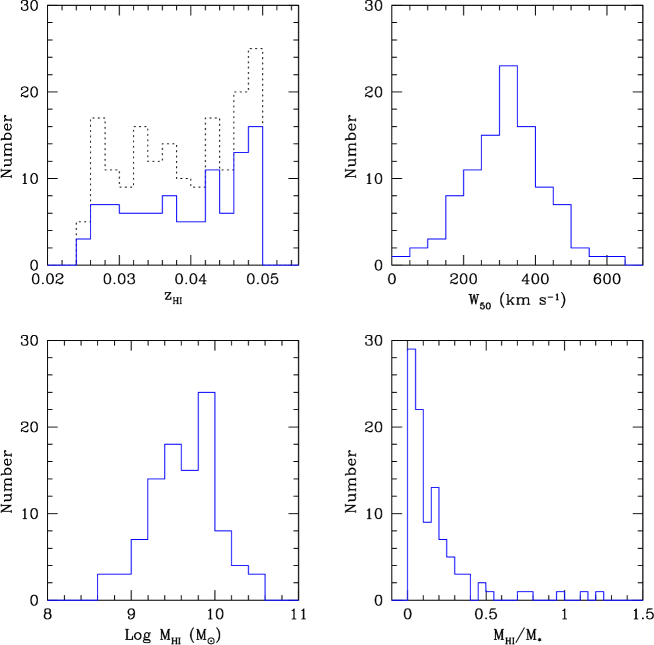
Figure 6: Distributions of redshifts, velocity widths, Hi masses and gas mass fractions for the 99 galaxies with Hi detections. The dotted histogram in the top left panel shows the distribution of SDSS redshifts for the full DR1 sample (i.e., including the non-detections).

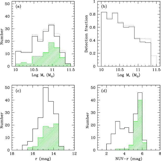
Figure 7: Stellar mass (a), SDSS r-band (c) and observed NUV$-r$ colour (d) distributions for the GASS DR1 sample (solid). Hatched histograms indicate the corresponding distributions for the non-detections. The detection fraction (i.e., the ratio of detections to total) is shown as a function of stellar mass in (b). The dotted histograms in the top panels are the average distributions for the representative sample discussed in the text (§ 7.2).

An overview of some of the optical- and UV-derived parameters for this data set is found in Figure 7, where solid and hatched histograms represent full sample and non-detections, respectively (dotted histograms will be discussed in the next section). Galaxies that were not detected in Hi are spread throughout the entire GASS stellar mass interval (panel a), but are preferentially found at higher $M_{\star}$ values. The detection rate of the survey as a function of $M_{\star}$ is shown in panel (b). The fraction of detected galaxies decreases with stellar mass, but does not drop below 35% even at stellar masses larger than $10^{11}$ M_⊙ (except for the very last bin, where we targeted only two objects). Thus, GASS is sensitive enough to detect Hi in a significant fraction of massive systems. The bottom panels of Figure 7 show SDSS r-band magnitude and observed (i.e., not corrected for dust attenuation) NUV$-r$ colour distributions for this sample. The well-known separation between blue cloud and red sequence galaxies, best appreciated when UV-to-optical colours are used (e.g., Wyder et al., 2007), is clearly seen in panel (d). Not surprisingly, nearly all the non-detections are found in the red sequence, whereas bluer, star-forming objects are almost always detected. Particularly interesting are the galaxies detected in red sequence. Of the 17 detections with NUV$-r$$>5$, half are highly inclined disks, thus their colours are likely reddened by dust, but most of the others have a featureless, spheroidal appearance in the SDSS images. The gas fractions of these detections are all below 6%, with two very notable exceptions, GASS 9863 and 3505 (Hi mass fractions of 27% and 50%, respectively), both early-type galaxies. GASS 3505 in particular is an extraordinary system that will be mentioned again in this work — its SDSS image and Arecibo detection can be seen in the left column of the second row of Figure 2.

Figure 8: The Hi mass fraction of the GASS sample is plotted here as a function of stellar mass, stellar mass surface density, concentration index, and observed NUV$-r$ colour. Red circles and green triangles represent detections and non-detections, respectively. Blue symbols indicate randomly selected, Hi-rich ALFALFA and S05 galaxies added to the DR1 sample in the correct proportion, to compensate for the fact that we do not re-observe objects with good detections in either of those archives. The sample including red, green and blue symbols is one example of the catalogs described in § 7.2, and contains 193 galaxies. For comparison, we also show the full set of ALFALFA galaxies meeting the GASS selection criteria that have been catalogued to date (gray). The stars in all plots highlight the locations of two interesting objects, GASS 3505 (red) and GASS 7050 (green), discussed in the text. The dashed line on the top-left panel indicates the Hi detection limit of the GASS survey. Dotted lines in each panel are linear fits to the red and blue circles only.

In Figure 8, we examine how the gas mass fraction of this sample varies as a function of several other galaxy properties. From top to bottom and from left to right, the Hi-to-stellar mass ratio is plotted as a function of stellar mass, stellar mass density, concentration index, and observed NUV$-r$ colour. In all panels, GASS detections are represented by red circles, and upper limits for non-detections are plotted as green, upside-down triangles. For comparison, the Hi-rich ALFALFA detections in the GASS parent sample are shown as small gray circles. Blue circles are randomly-selected, gas-rich galaxies from either ALFALFA or the S05 archive of pointed observations, added to the DR1 sample in the right proportion to quantify average trends in the data (see § 7.2). The stars identify the locations of GASS 3505 (red) and GASS 7050 (green), which are somewhat extreme examples of two opposite types of transition galaxies. The former is an early-type galaxy with unusually high gas content that might be reaccreting a disk (thus moving from the red toward the blue sequence), and the latter is a gas-poor, disk galaxy (which is likely moving in the opposite direction, from the blue to the red sequence. The SDSS image and Hi spectrum of GASS 7050 can be seen in the right column of the second row of Figure 4). This figure illustrates how GASS is able to measure the Hi content of massive galaxies down to a gas fraction limit which is an order of magnitude lower than that achieved by ALFALFA over the same redshift range. This allows us to quantify the distribution of atomic gas fractions over a much wider dynamic range. The figure also illustrates the relative strengths of the correlations (or lack thereof) between gas content and galaxy structural parameters, and also between gas content and NUV$-r$, a quantity that characterizes the stellar populations of the galaxies in our sample.

We discuss each panel below. In order to quantify the scatter in each correlation, we have performed a least-squares fit to all the galaxies with Hi detections (i.e., all the points plotted as red and blue circles in Fig. 8). The result of the fit is shown as a dotted line in each panel. We only report the rms variance in Log $M_{\rm HI}$/$M_{\star}$ about each relation, $\sigma$, in the text below.

Stellar mass. — The apparently clean correlation between gas mass fraction and $M_{\star}$ exhibited by the Hi-rich ALFALFA galaxies in this stellar mass regime is mostly due to the sensitivity limits of the blind Hi survey. At each stellar mass, GASS detects many objects with significantly lower gas fractions. The gas fraction of the GASS detections decreases as a function of stellar mass, but the correlation has larger scatter ($\sigma=0.386$ dex) compared to the one obtained for the ALFALFA galaxies. As already noted, the non-detections span the full $M_{\star}$ interval studied by GASS, but their fraction of the targeted sample increases with stellar mass. The stellar mass-dependent detection limit of our survey is indicated by a dashed line.

Stellar mass density. — Interestingly, the gas content of massive galaxies seems to correlate better with $\mu_{\star}$ than with $M_{\star}$. Quantitatively, the rms variance in Log $M_{\rm HI}$/$M_{\star}$ at a fixed value of $\mu_{\star}$ is $\sigma=0.364$ dex, i.e. 6% smaller than the variance at a fixed value of $M_{\star}$. Another striking feature in this plot is the distribution of the non-detections, which all have $\mu_{\star}$$>10^{8.6}$ M_⊙ kpc^-2, without a single exception. We will come back to this point later.

Concentration index. — The concentration index is defined as $R_{90}/R_{50}$, where $R_{90}$ and $R_{50}$ are the radii enclosing 90% and 50% of the r-band Petrosian flux, respectively (see Table 1). As shown in Figure 1 of Weinmann et al. (2009), there is a tight and well-defined correlation between the concentration index and the bulge-to-total ratio derived from full 2-dimensional multi-component fits using the methods presented in Gadotti (2009). It is thus very interesting that the dependence of $M_{\rm HI}$/$M_{\star}$ ratio on concentration is considerably weaker ($\sigma=0.449$ dex) than its dependence on stellar mass or stellar surface density. Because the Hi gas is expected to be located in the disk and not the bulge, this lack of correlation might imply that the bulge has little influence on the formation or fuelling of the disk.

NUV$-$r colour. — Colour is well known to be a reasonably good predictor of gas content for blue-sequence, star-forming galaxies. We show here that the correlation between those two quantities continues with increased scatter beyond the blue sequence traced by the Hi-rich ALFALFA galaxies, and down to the survey gas fraction limit. This is in agreement with previous work by, e.g., Cortese & Hughes (2009), based on a sample of galaxies located in regions in and around nearby clusters. Among the four parameters considered here (i.e., $M_{\star}$, $\mu_{\star}$, $R_{90}/R_{50}$ and NUV$-r$), NUV$-r$ colour is the one most tightly correlated with gas fraction ($\sigma=0.327$ dex). As seen in Figure 7d, almost all the non-detections are found in the red sequence. We also notice that GASS 3505 and GASS 7050 stand out as clear outliers in this plot, with a gas content well displaced from the average for their NUV$-r$ colour.

In the remainder of the paper, we will quantify the main correlations explored in this section and discuss their implications.

7.2 Building a Representative Sample

Although this first data release amounts to only $\sim$20% of the full survey sample, our target selection has not been biased by any galaxy property except stellar mass. As described in § 3, in this initial phase of the survey we have given some priority to galaxies with stellar masses greater than $10^{10.5}$ M_⊙, but otherwise the selection has been random. We can thus use this sample to quantify the correlations between Hi mass fraction and other physical parameters discussed above, after accounting for the missing Hi-rich objects that were not observed because they are in ALFALFA or in the S05 archive.

In order to construct a sample of galaxies that is representative in terms of Hi properties, we clearly need to add the correct proportions of ALFALFA and S05 galaxies to the GASS data set. We determined such proportions for each stellar mass bin as follows. We used the ALFALFA catalog footprint available to date to estimate the fractions of GASS parent sample galaxies detected by ALFALFA ($f_{\rm AA}$) and in the S05 archive ($f_{\rm S05}$, not counting those already in $f_{\rm AA}$). One complication is that we observed targets outside that footprint, some of which might turn out to be ALFALFA detections, and we should not count these twice. Thus, let us call $N_{\rm G}$ and $N_{\rm G,<AA}$ the total number of GASS objects in the given stellar mass bin and those below the ALFALFA detection limit, respectively. The numbers of ALFALFA and S05 galaxies that should be added back into the sample, for each stellar mass bin, are:

$$N_{\rm AA}=\frac{N_{\rm G,<AA}}{1-f_{\rm AA}}\times f_{\rm AA}-(N_{\rm G}-N_{\rm G,<AA}),$$

where ($N_{\rm G}-N_{\rm G,<AA}$) effectively count as ALFALFA detections (they would be if that survey was already completed), and

$$N_{\rm S05}=\frac{N_{\rm G,<AA}}{1-f_{\rm S05}}\times f_{\rm S05},$$

where, as noted above, $f_{\rm S05}$ does not include ALFALFA detections. Repeating this process for each stellar mass bin yields a sample of $\sim$200 galaxies.

In order to better account for statistical fluctuations, we generated 100 such catalogs, each time selecting objects randomly from the ALFALFA and S05 data sets in the correct proportions. More specifically, each catalog is obtained by adding $N^{\prime}_{\rm AA}$ and $N^{\prime}_{\rm S05}$ galaxies to each $M_{\star}$ bin of the GASS data set, where $N^{\prime}_{\rm AA}$ and $N^{\prime}_{\rm S05}$ are random Poisson deviates of $N_{\rm AA}$ and $N_{\rm S05}$, respectively. The catalogs contain between 179 and 193 galaxies (187 on average), thus the percentage of Hi-rich galaxies added to the GASS sample is less than 10%. This is illustrated by the blue symbols in Figure 8 for one of these catalogs (red and green symbols are GASS detections and non-detections, respectively, and blue circles are randomly-selected Hi-rich galaxies that were added to each $M_{\star}$ bin).

When we compute the average Hi gas fraction as a function of different galaxy properties, we do so based on the 100 catalogs discussed here. The average data set obtained from these catalogs will be referred to henceforth as our representative sample. To estimate error bars, we also tried to take into account the variance internal to the GASS sample itself using standard bootstrapping techniques. We generated 100 random catalogues in a similar way to that described above, but we also draw random indices for GASS galaxies (allowing for repetitions). The catalogs in this second set include between 179 and 200 galaxies each (189 on average).

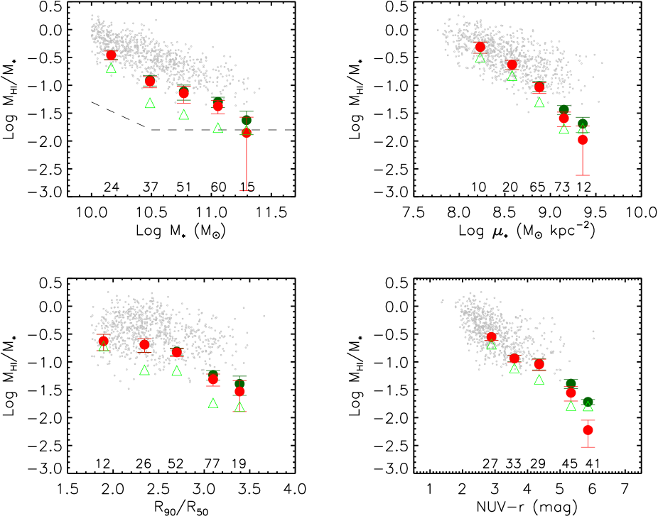
Figure 9: Average trends of Hi mass fraction as a function of stellar mass, stellar mass surface density, concentration index and observed NUV$-r$ colour based on the representative sample discussed in § 7.2. In each panel, large circles indicate average gas fractions (weighted as explained in the text). These were computed including the non-detections, whose Hi mass was set to either its upper limit (dark green) or to zero (red). Green triangles are weighted medians. The average number of galaxies in each bin, $N_{\rm i}$, is indicated above the x axis; only bins with $N_{\rm i}\geq 8$ are shown. These results are listed in Table 4. Galaxies in the GASS parent sample detected by ALFALFA are plotted as small gray circles. The dashed line in the first panel shows the Hi detection limit of the GASS survey.

7.3 Gas Fraction Scaling Relations

In Figure 9, we show how the average Hi mass fraction of massive galaxies varies as a function of stellar mass, stellar mass surface density, concentration index and observed NUV$-r$ colour. This quantity is calculated for each of the 100 catalogs described in the previous section that do not include bootstrapping of the GASS galaxies. We average the gas fractions in a given bin, properly weighted in order to compensate for the uneven stellar mass sampling of the DR1 data set, using the full GASS parent sample as a reference. We bin both the parent sample and the individual catalogs by stellar mass (with a 0.2 dex step), and use the ratio between the two histograms as a weight. In other words, a galaxy in the $i$-th stellar mass bin and in a given catalog is assigned a weight $N_{{\rm PS},i}/N_{{\rm cat},i}$, where $N_{{\rm PS},i}$ and $N_{{\rm cat},i}$ are the numbers of objects in the $i$-th Log $M_{\star}$ bin in the parent sample and in that catalog, respectively. This is a valid procedure because the parent sample is a volume-limited catalogue of galaxies with $M_{\star}$$>10^{10}$ M_⊙. The final average gas fractions are then computed by averaging the weighted mean values obtained for each catalog. The results are shown as large circles in Figure 9. The difference between green and red circles illustrates two different procedures for dealing with the non-detections: the Hi mass is set either to the upper limit (green) or to zero (red). As can be seen, the answer is insensitive to the way we treat the galaxies without Hi detections, except for the very most massive, dense and red galaxies. Note that this is entirely due to the deep limit of the GASS survey. The error bar on each circle indicates the 1$\sigma$ uncertainty on our estimate of the average gas mass fraction, computed from the dispersion of the weighted mean values of the bootstrapped catalogs. The average number of galaxies that contributed to each bin is indicated in the panels. Because of the small number statistics in some of these bins, our bootstrapping analysis might still underestimate the error bars.

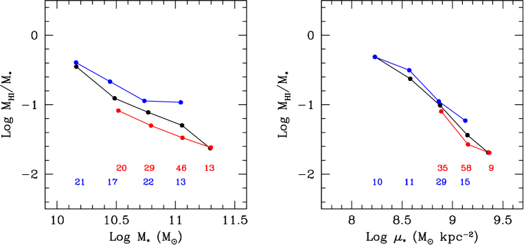
Figure 10: Gas fraction as a function of stellar mass and stellar mass density for our representative sample. Black symbols and lines are weighted averages obtained by setting the non-detections to their upper limits (same as dark green trends in Fig. 9). Left: The sample is divided into two bins of stellar mass density (blue: Log $\mu_{\star}$$<8.9$, red: Log $\mu_{\star}$$\geq 8.9$). Right: The sample is divided into two bins of stellar mass (blue: Log $M_{\star}$$<10.7$, red: Log $M_{\star}$$\geq 10.7$). Average numbers of galaxies in each bin are indicated in the panels. Only averages based on $N\geq 9$ galaxies are plotted.

Weighted median values of the $M_{\rm HI}$/$M_{\star}$ ratios are plotted in Figure 9 as triangles. In the highest $M_{\star}$, $\mu_{\star}$, concentration index and NUV$-r$ colour bins, the “median” galaxy is a non-detection. The values of weighted average and median gas fractions illustrated in this figure are listed in Table 4 for reference. Lastly, small gray circles in these panels represent galaxies in the GASS parent sample detected by ALFALFA. It is clear that the shallower, blind Hi survey is biased to significantly higher gas fractions compared to our estimates of the global average.

As the plots in Figure 9 and Table 4 show, the gas content of massive galaxies decreases with increasing $M_{\star}$, $\mu_{\star}$ concentration index, and observed NUV$-r$ colour. The strongest correlations are with $\mu_{\star}$ and NUV$-r$. The average gas fraction decreases by more than a factor of 30 as $\mu_{\star}$ increases from $10^{8}$ M_⊙ kpc^-2 to a few times $10^{9}$ M_⊙ kpc^-2, i.e. the relation is very close to a linear one. A similar large decrease is obtained as a function of NUV$-r$. In contrast, the average Hi fraction decreases by a factor of $\sim$20 over a 1.5 dex range in stellar mass. The relation with concentration index is even shallower, remaining approximately constant up to a concentration index of 2.5, and then declining by a factor of only $\sim$5 up to the highest values of $R_{90}/R_{50}$. Figure 9 also shows that the difference between the mean and median values of $M_{\rm HI}$/$M_{\star}$ is smallest when it is plotted as a function of $\mu_{\star}$ and NUV$-r$. This is because these two properties yield relatively tight correlations without significant tails to low values of gas mass fraction (see Fig. 8).

In Figure 10, we split our sample into two bins in stellar mass density (left) and in stellar mass (right). Although somewhat limited by small number statistics, there is evidence that a change in $M_{\star}$ has a smaller effect on the relation between gas fraction and $\mu_{\star}$ than viceversa. In other words, the gas mass fraction of massive galaxies appears to be primarily correlated with $\mu_{\star}$, and not $M_{\star}$.

Finally, in Figure 11, we have plotted the fraction of galaxies with Hi gas fractions greater than 0.1 (squares) and greater than 0.03 (circles) as a function of stellar mass and stellar surface density. As can be seen, the fraction of galaxies with significant (i.e., more than a few percent) gas decreases smoothly as a function of stellar mass. In contrast, there appears to be a much more sudden drop in the fraction of such galaxies above a characteristic stellar surface density of $3\times 10^{8}$ M_⊙ kpc^-2. This result can also be seen in the top right panel of Figure 8, where we see that all the galaxies that were not detected in Hi have stellar surface densities greater than $3\times 10^{8}$ M_⊙ kpc^-2.

Figure 11: Detection fraction of galaxies as a function of stellar mass (left) and stellar mass surface density (right). Circles and squares represent objects with $M_{\rm HI}$/$M_{\star}$ greater that 3% and 10%, respectively.

7.4 Predicting the Hi Fraction

As discussed in the previous sections, the Hi mass fraction is most tightly correlated with stellar surface mass density and NUV$-r$ colour, and the correlations are close to linear (at least for galaxies on the blue sequence). In addition, it can be demonstrated that there is also a tight correlation between NUV$-r$ colour and stellar surface mass density. This implies that a linear combination of the two latter quantities might provide us with an excellent predictor for the average gas content of a massive galaxy. We have thus fit a plane to the 2-dimensional relation between Hi mass fraction, stellar surface mass density, and NUV$-r$ colour following the methodology outlined in Bernardi et al. (2003). This is standard practice for elliptical galaxies, which have been shown to obey a tight plane in the 3-dimensional space of effective radius, surface brightness and stellar velocity dispersion.

We performed this plane-fitting exercise using only detected galaxies in one of the non-bootstrapped catalogs described in § 7.2 (the one illustrated in Figure 8). The sample used is reproduced in Figure 12, where red and blue circles indicate DR1 detections and Hi-rich objects added to the sample, respectively. ALFALFA galaxies (small circles) and non-detections (upside-down triangles) are not used in the fit and are shown for comparison only. The gas fractions obtained from our best fit relation are compared with measured ones in the figure. The 1:1 relation is indicated by a dotted line, and the values of the fit coefficients are given in the caption. The rms scatter in Log $M_{\rm HI}$/$M_{\star}$ about this relation is 0.315 dex, i.e., we obtain a 4% and 13% reduction in the scatter compared to the 1-d relations involving NUV$-r$ and $\mu_{\star}$, respectively.

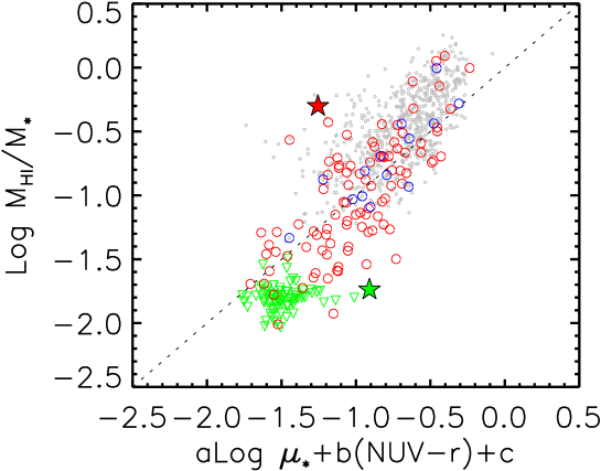
Figure 12: The best fit “plane” describing the relation between Hi mass fraction, stellar mass surface density and observed NUV$-r$ colour is plotted as a dotted line. All the symbols are the same as those in Fig. 8. The values of the coefficients listed above are the following: $a=-0.332,~{}b=-0.240,~{}c=2.856$.

We note that the most gas-rich galaxies in our sample, as well as the ALFALFA galaxies, lie systematically above the plane, as expected. The most gas-poor galaxies lie systematically below the plane. This may result from the fact that the non-detections are not used in the fit. With the increased sample sizes that will be available to us in future, we will be able to stack the non-detections to estimate an average gas content, and attempt to use this measurement as a way to anchor the prediction at the low gas fraction end.

Perhaps the most interesting use for our best-fit plane is as a means to identify interesting objects that deviate strongly from the average behavior of the sample. These outliers are the best candidates for galaxies that might be transitioning between the blue cloud of star-forming spirals and the red sequence of passively-evolving galaxies.

Galaxies which are anomalously gas-rich given their colours and densities scatter above the mean relation, while those that are gas-poor scatter below. This is clearly demonstrated by the Hi-rich ALFALFA galaxies, which are preferentially found above the line. Also, GASS 3505 (marked with a red star on the diagram), a galaxy that has optical morphology and colours characteristic of a normal elliptical, but a 50% Hi mass fraction, is a clear outlier in this plane.

Of equal interest are the galaxies with low Hi mass fractions, but that are still forming stars. These galaxies are found near the bottom the plots, but shifted to the right (e.g., GASS 7050, a gas-poor disk galaxy that was not detected in Hi, is indicated by a green star). These may be systems where the Hi gas has recently been stripped by tidal interactions or by ram-pressure exerted by intergalactic gas, or where other feedback processes have expelled the gas. In future work, we plan to investigate these different classes of transition galaxy in more detail.

8 Summary and Discussion

In this paper we introduce the GALEX Arecibo SDSS Survey (GASS), an on-going large program that is gathering high quality Hi-line spectra for an unbiased sample of $\sim$1000 massive galaxies using the Arecibo radio telescope. The sources are selected from the SDSS spectroscopic and GALEX imaging surveys, and have stellar masses $M_{\star}$$>10^{10}$ M_⊙ and redshifts $0.025<z<0.05$. They are observed until detected or until a low gas mass fraction limit (1.5$-$5% depending on stellar mass) is reached.

Blind Hi surveys such as ALFALFA, which detects $\sim$20% of the GASS targets, are heavily biased towards blue, gas-rich systems at the same redshifts. A number of past studies have investigated the Hi content of elliptical and early-type galaxies (e.g., Morganti et al., 2006; Oosterloo et al., 2007), but these samples are selected by morphology and hence may not be representative of the full population of massive galaxies. GASS is the first study to specifically target a sample that is homogeneously selected by stellar mass, a robust measure that is essential for understanding the observations and connecting them with theory.

We have presented the first Data Release, DR1, consisting of $\sim$20% of the final GASS sample. Based on this first data installment we have built an unbiased, representative sample, which has been used to explore the main scaling relations between Hi gas fraction and other parameters related to structure and stellar populations of the galaxies in this study. Our main findings are discussed below.

1. A large fraction ($\sim$60%) of the galaxies are detected in Hi. Even at stellar masses above $10^{11}$ M_⊙, the detected fraction does not fall below $\sim$40%. Around 9% of galaxies more massive than $10^{11}$ M_⊙ have Hi fractions larger than 0.1 and 34% have Hi fractions larger than 0.03.

2. We have studied the correlation between $M_{\rm HI}$/$M_{\star}$ ratio and a variety of different galaxy properties. We find that the gas fraction of massive galaxies correlates strongly with stellar mass, stellar surface mass density and NUV$-r$ colour, but correlates only weakly with the concentration index of the r-band light. The scatter in the correlations increases visibly outside the blue sequence of Hi-rich, star-forming spirals.

3. The gas content of massive galaxies decreases for increasing values of $M_{\star}$ and $\mu_{\star}$. The latter quantities are clearly related, but we presented evidence (although based on somewhat limited statistics) that the primary correlation is with stellar mass surface density, rather than with stellar mass.

4. We also found that the fraction of galaxies with significant gas content (i.e., $M_{\rm HI}$/$M_{\star}$ greater than a few percent) decreases strongly above a stellar surface mass density of $10^{8.5}$ M_⊙ kpc^-2. This is the threshold stellar mass density between disk-dominated, late-type galaxies and bulge-dominated, early-type objects identified by Kauffmann et al. (2006), across which the recent star formation histories of local galaxies have been shown to undergo a transition. Based on their study of the scatter in colour and spectral properties of SDSS galaxies, Kauffmann et al. argue that star formation proceeds at the same average rate per unit stellar mass below the characteristic surface density, and shuts down above the threshold. Schiminovich et al. (2007) also noted a striking change in the UV-derived specific SFRs of SDSS galaxies at the same characteristic $\mu_{\star}$ (see their Fig. 20).

5. A similar transition in gas properties near the characteristic stellar mass $M_{\star}$$\sim$3 $\times$$10^{10}$ M_⊙ (Strateva et al., 2001; Kauffmann et al., 2003; Baldry et al., 2004) is not evident from our data. This appears to be in contradiction to the results of Bothwell, Kennicutt & Lee (2009), who claim to detect such a transition in $M_{\rm HI}$/$M_{\star}$, based on a sample of much more nearby galaxies. We caution that our results are still limited by small statistics, particularly at the low stellar mass end.

One of the key goals of the GASS survey is to identify and quantify the incidence of transition objects, which might be moving between the blue, star-forming cloud and the red sequence of passively-evolving galaxies. Depending on their path to or from the red sequence, these objects should show signs of recent quenching of star formation or accretion of gas, respectively. This task requires us to establish the normal gas content of a galaxy of given mass, structural properties and star formation rate. The classic concept of Hi deficiency established for spiral galaxies (Haynes & Giovanelli, 1984; Solanes, Giovanelli, & Haynes, 1996) is a well-known attempt to quantify whether or not a galaxy has been recently stripped of its Hi gas. Our approach is to fit a plane to the 2-dimensional relation between Hi mass fraction, stellar surface mass density, and NUV$-r$ colour. We showed preliminary results that make use of Hi detections only, and will include non-detections at a later stage, when we have larger samples that will allow us to recover a signal from their stacked spectra.

The GASS survey has already identified a few interesting examples of transition galaxies. In this work we have pointed out two examples, GASS 3505 and GASS 7050, i.e., a very gas-rich, early-type galaxy and a gas-poor disk. Many examples of Hi-deficient galaxies are known from the literature. More intriguing are red sequence galaxies that might be accreting gas and maybe even regrowing a disk (such as perhaps GASS 3505). Two such systems, NGC 4203 and NGC 4262, have been identified by Cortese & Hughes (2009) from a more local sample of galaxies. The authors report convincing evidence that the Hi, which is distributed in ring-like structures in both NGC objects, might be of external origin. Interestingly, also GASS 3505 shows an external ring-like structure in the GALEX images. We have recently obtained VLA data for this galaxy, and will report on it in a separate paper.

The GASS data base of stellar and gas-dynamical measurements will provide an unprecedented view of the gas properties and kinematics of massive galaxies, complementing the results of on-going blind surveys such as ALFALFA. Once completed, GASS will allow us to move beyond the mean gas fraction scaling relations studied in this paper, and address second order questions, such as how the gas fractions depend on metallicity or other quantities at fixed stellar mass. GASS will also quantify the frequency with which different kinds of transition galaxies occur in the local universe, and how this depends on factors such as local environment and AGN content. Insight into the nature of massive and transition objects will give us a strong foundation to further understand the gas properties of high-redshift galaxies, and will help guide future directions for Hi surveys at existing and planned radio facilities.

Appendix: Notes on Individual Objects

We list here notes for galaxies marked with an asterisk in the last column of Tables 2 and 3. The galaxies are ordered by increasing GASS number. In what follows, AA1 and AA2 are abbreviations for ALFALFA detection codes 1 and 2, respectively.

Detections (Table 2)
3261 – detected on top of weak RFI across all band; AA1.
3504 – detected on top of weak RFI across all band; low frequency edge uncertain, systematic error.
3645 – detected on top of weak RFI across all band; AA2.
3777 – detected on top of RFI across all band; AA2.
3817 – hints of RFI across band; AA1.
3962 – disk $\sim$1.5′ N has z=0.027, no contamination problems; blue spiral $\sim$3′ E, z=0.0314 (1377.16 MHz), detected in board 4. Low frequency edge uncertain, systematic error.
3971 – hints of RFI across band in one pair; AA2; low frequency edge uncertain, systematic error.
6375 – group: 2 blue galaxies 2.7′ away, GASS 6373 (= VCC 1016, spiral, similar size) to the S and SDSS J122716.82+031812.9 (smaller) to the W, same cz. The two spirals do not look distorted and the Hi profile is not clearly confused, just slightly offset in z (but notice that GASS 6373 is offset in the wrong direction). Contamination likely.
6506 – GASS 6501, red galaxy $\sim$3′ away, 1355.75 MHz not detected; RFI spike at 1350 MHz.
7025 – high frequency peak uncertain.
7493 – GASS 7457 (non-detection) $\sim$1′ away, no contamination problems (z=0.026; GASS 7457 has z=0.036); uncertain profile, systematic error; SDSS emission line z (0.02622) in better agreement with Hi.
7509 – small satellites, some contamination very likely; stronger in polarization A; high frequency edge uncertain, systematic error.
9343 – 2 blue galaxies within 1′, no cz, possible contamination; poor fits to edges.
9463 – merger, plus another blue galaxy $\sim$1′ away with same z: confusion certain; very uncertain Hi profile, systematic error.
9514 – smaller disk galaxy $\sim$1′ away, same z, some contamination likely; AA2; poor fit to low frequency edge.
9619 – blue, disrupted little galaxy $\sim$3′ away, same z, some contamination possible.
9776 – small blue disk $\sim$15″ away, same cz (z=0.027568, 1382.30 MHz), some contamination certain. Looks like the edges of the Hi profile come from 9776, but the central peak is dominated by the companion.
9814 – blue smudges nearby + small galaxy $\sim$1.5′ NW, same cz; possible contamination; low frequency peak uncertain.
10019 – RFI spike near 1375.3 MHz, slightly drifting in frequency.
10132 – two small companions: a blue one $\sim$1.3′ N, strong $\rm H\alpha$ emission in SDSS spectrum, z=0.0438 (1360.80 MHz), and a galaxy $\sim$1.5′ E, no $\rm H\alpha$  in SDSS spectrum, z=0.0444 (GASS 10132 has z=0.0443). The strong peak in the Hi spectrum is centered on the blue companion. Blend.
11016 – galaxy pair: 11016 is a red gal, no emission lines in SDSS spectrum, centered at 1369.07 MHz, the companion is a blue galaxy 1.2′ SE, strong emission lines in SDSS spectrum, centered at 1368.93 MHz. Confusion certain.
11223 – small early type $\sim$40″ away, no cz, small contamination possible; poor fit to high frequency edge; AA2.
11386 – small peak outside Hi profile (on the high frequency side) is mostly in polarization B.
11956 – companion also detected (SDSS J000814.67+150752.9, z=0.0372, 1369.46 MHz, blue disk 2.1′ SW), no overlap.
11989 – small blue galaxy 2′ away, no cz, but confusion unlikely. High frequency edge uncertain, systematic error; AA4 (i.e., classified by ALFALFA as tentative detection with optical counterpart of unknown redshift).
12371 – 3 blue galaxies within 3′, no contamination problems (largest one has z=0.008, other two have z=0.027 and are detected in board 4 (1383 MHz).
12983 – low frequency edge uncertain, systematic error.
13227 – stronger in polarization B; uncertain profile, poor fit to high frequency edge, systematic error.
14831 – small galaxies nearby (within $\sim$1′), no cz; some contamination possible; high frequency edge uncertain, systematic error.
15181 – AA1.
17640 – AA2.
18279 – confused or blend: most of the signal comes from blue galaxy $\sim$1.5′ away, z=0.0492 (1353.80 MHz); 2 other galaxies within 2′ have very different z (0.18 and 0.07).
18421 – stronger in polarization B.
18581 – low frequency peak uncertain.
20133 – galaxy pair: GASS 20165 $\sim$1′ away, z=0.0498 (1353.04 MHz; GASS 20133 has z=0.0489, 1354.19 MHz); however 20165 is a red, early type gal, not detected in 10m on-source, so significant contamination is unlikely.
20144 – uncertain profile edges, systematic error.
20286 – RFI at 1376 MHz.
23315 – blue disk $\sim$1′ away has z=0.054, no contamination; low frequency edge uncertain, systematic error.
23445 – 2 galaxies at $\sim$2.7′: one at N has z=0.08, one at W is small, has $\sim$same cz (z=0.047065, 1356.56 MHz) and is not detected in spectrum (a bit offset so should be visible if there); better in polarization B; uncertain profile.
24740 – uncertain profile, systematic error.
26822 – AA2.
28526 – RFI spike near 1354 MHz (within profile), 2 channels replaced by interpolation.
29487 – small companion 2.4′ S, z=0.0424 (1362.63 MHz, 0.5 MHz offset), contamination possible but unlikely; strong, narrow RFI near 1359 MHz.
29505 – much stronger in polarization B; no trace of RFI, well centered on SDSS z.
29842 – AA2.
30175 – blue companion 1.6′ away, slightly lower z (z=0.0223, 1389.42 MHz) also detected. Two other galaxies $\sim$3′ away have z=0.08.
30401 – AA2.
31156 – AA2.
38462 – poor fits to edges.
38703 – stronger in polarization B.
38717 – narrow RFI at 1360 and 1370 MHz (no radar blanker).
38758 – small, blue companion $\sim$0.5′ away, no cz; galaxy clearly distorted, contamination very likely.
38964 – small satellite to the S? blue, edge-on galaxy $\gtrsim$ 3′ away, z=0.033468 (1.6 MHz away), not detected but might be responsible for asymmetry (raising low frequency peak).
39567 – GASS 39600 $\sim$2.5′ away to the N, no contamination problems (z=0.044, GASS 39567 has z=0.031); much stronger in polarization B.
39595 – AA2. Low frequency edge uncertain, systematic error.
40007 – galaxy pair (separation 1.3′, difference of recessional velocities is 60 km s^-1); 2 blue spirals, same cz, $\sim$3′ and 4.5′ away (group); Hi spectrum does not look confused but contamination certain (note z off with respect to SDSS redshift of both galaxies).
40024 – group: 3 small galaxies around (1′-3), 2 with $\sim$same cz, one without cz; some contamination likely; high frequency edge and peak uncertain, systematic error, poor fit.
40393 – uncertain peaks.
40494 – RFI spike near 1357 MHz (within profile), 3 channels replaced by interpolation.
40781 – strong RFI spike at 1356 MHz (within profile), 4 channels replaced by interpolation.
41969 – AA1.
41970 – small disk galaxy 10″ to the W, contamination possible (perhaps higher z, though).
42015 – AA2.
42167 – 3 disks within 2′-4′ have different z (largest one at $\sim$4′, 1373.17 MHz, not detected), no contamination problems.
47221 – low frequency edge uncertain, systematic error (little side peak is in polarization B only).
47405 – high frequency edge uncertain, systematic error.

Non-detections (Table 3)
7286 – small companion $\sim$1.5′ away, same z.
7457 – see GASS 7493 (detection).
9507 – RFI spike at 1352 MHz.
9891 – blue disk $\sim$2.5′ away, z=0.0243 (1386.71 MHz) not detected.
10150 – galaxy $\sim$1′ away has z=0.092, no contamination problems.
10358 – group (3 galaxies $\sim$same cz within 3′).
10367 – group (3 galaxies $\sim$same cz within 1.5′-4′).
10404 – small blue galaxy 20″ E, no cz, responsible for small spike at 1369.3 MHz?.
12455 – group: 2 other galaxies at 2.5′ W and 3.5′ E, $\sim$same cz; marginally detected the one at 2.5′ (small edge-on disk, z=0.0484, 1354.83 MHz)?.
12458 – RFI spike at 1370.2 MHz.
12460 – RFI spike at 1350.8 MHz. Detected blue companion (irregular galaxy $\sim$1′ away, no cz) at 1352.2 MHz? Not seen RFI there, but much stronger in polarization B.
13156 – AA2.
13549 – group: several small gals, $\sim$same z, within 3′; also a larger early type, no cz.
18422 – small galaxy $\sim$1.3′ W, no cz (+ other, smaller ones).
21023 – RFI at 1358-59 MHz, slightly drifting in frequency.
25154 – galaxy pair, companion is a spiral $\sim$1′ away, optical em lines, z=0.0364 (1370.52 MHz), also not detected.
25214 – group (4 galaxies $\sim$same cz within 3′).
25575 – galaxy pair (galaxy $\sim$same cz 20″ W).
26958 – disturbed morphology, merger? marginally detected companion (blue disk $\sim$0.5′ away, no cz)?.
29090 – detected blue edge-on disk $\sim$3′ S; 3 other disks $\sim$3′-4′ away.
29420 – group: two small galaxies $\sim$2′ away, same cz, + others, no cz; looks like a galaxy is detected in the off.
29699 – group: 2 galaxies $\sim$same z within 2′, and another one at z=0.044.
30479 – disk $\sim$1.5′ away has z=0.08, no contamination problems.
38472 – blue galaxy $\sim$1′ SW has z=0.202, no contamination problems.
39448 – blue galaxy $\sim$1′ away, same cz (z=0.0341; GASS 39448 has z=0.0339), contamination certain.
39465 – blue irregular galaxy $\sim$1′ NW detected in board 3; galaxy $\sim$1′ SW has z=0.076; 2 galaxies $\sim$0.5′ SW, no cz, marginally detected?.
39606 – $\sim$3′ away from GASS 39607, same cz, also not detected.
39607 – see GASS 39606.
40257 – group: 3 small galaxies within 2.5′ E and a large disk $\sim$2′ NW, $\sim$same cz.
40317 – group: 3 galaxies within 2.5′, $\sim$same cz; marginally detected blue irregular, 2′ SW, z=0.0404 (1365.25 MHz)?.
40686 – group: 4 galaxies within 2′, $\sim$same cz, one detected (SDSS J131527.88+095243.7, a bluish, edge-on disk $\sim$2′ away, z=0.0505, 1352.12 MHz).
40790 – small companion $\sim$1′ away, z=0.0499 (1352.90 MHz), also not detected.
41974 – group in background (3 galaxies at 2′-3′ with z=0.045-0.047), no contamination problems.
42020 – blue irregular galaxy nearly attached, no cz; neg. spike near 1373 MHz is not RFI and is in both pols… galaxy in off?.
42156 – detected SDSS J151719.24+072828.3, a blue disk $\sim$1.5′ SW, z=0.0367 (1370.16 MHz). Possible contribution from GASS 42164 at the same cz (1370.03 MHz), a larger, face-on, red spiral $\sim$2′ away from GASS 42156. Also, small disk, 2′ E, z=0.077. No confusion problems.

Table 1: SDSS and UV Parameters of the GASS Galaxies.

			Log $M_{\star}$	$R_{50,z}$	$R_{50}$	$R_{90}$	Log $\mu_{\star}$	extr	r	NUV$-r$	TNUV	$T_{\rm max}$
GASS	SDSS ID	$z_{\rm SDSS}$	(M⊙)	(″)	(″)	(″)	(M⊙ kpc-2)	(mag)	(mag)	(mag)	(sec)	(min)
(1)	(2)	(3)	(4)	(5)	(6)	(7)	(8)	(9)	(10)	(11)	(12)	(13)
11956	J000820.76+150921.6	0.0395	10.09	2.99	3.10	6.68	8.48	0.16	16.28	3.04	1680	90
12025	J001934.54+161215.0	0.0366	10.84	3.67	3.92	11.86	9.13	0.18	14.74	5.93	4835	14
11989	J002558.89+135545.8	0.0419	10.69	2.53	2.66	8.02	9.18	0.22	15.14	5.79	3344	47
3261	J005532.61+154632.9	0.0375	10.08	2.84	3.03	7.70	8.57	0.26	15.49	2.63	1918	72
3645	J011501.75+152448.6	0.0307	10.33	3.07	3.22	8.74	8.93	0.17	15.12	3.97	1440	32
3505	J011746.76+131924.5	0.0479	10.21	1.90	1.99	6.56	8.83	0.10	16.35	4.92	1647	198
3504	J011823.44+133728.4	0.0380	10.16	6.53	8.53	15.68	7.91	0.11	15.34	2.85	1647	76
3777	J012316.81+143932.4	0.0396	10.26	2.68	2.87	6.35	8.75	0.14	15.69	3.17	1654	90
3817	J014325.96+135116.8	0.0450	10.07	3.94	4.38	10.70	8.11	0.18	15.76	2.36	3361	153
4239	J015816.23+141747.9	0.0261	10.80	4.64	5.14	17.23	9.18	0.15	13.92	5.58	1663	4
3962	J020359.14+141837.3	0.0427	10.90	4.66	5.26	15.46	8.84	0.19	14.51	3.22	1664	19
3971	J020552.48+142516.2	0.0426	10.43	3.85	4.38	11.99	8.54	0.19	15.82	3.33	1645	122
57017	J092229.28+142743.3	0.0323	10.54	3.04	3.95	12.16	9.10	0.09	16.22	4.00	2857	33
20133	J093236.58+095025.9	0.0489	10.86	4.38	4.81	11.05	8.73	0.11	14.69	…	…	42
20144	J093502.01+095512.4	0.0496	10.06	3.76	4.08	7.39	8.06	0.08	16.27	2.54	106	229
20286	J095439.45+092640.7	0.0346	10.53	3.59	3.88	10.21	8.89	0.10	15.74	4.11	3178	44
14831	J100530.26+054019.4	0.0444	11.21	4.60	5.00	13.62	9.13	0.05	14.59	4.25	299	5
14943	J101600.20+061505.2	0.0458	11.33	4.56	4.85	16.36	9.23	0.06	13.74	6.44	330	4
18900	J102001.61+083053.6	0.0453	10.92	2.72	2.62	8.28	9.28	0.08	14.63	5.39	6825	23
22999	J102316.42+115120.4	0.0455	10.64	4.20	4.65	9.77	8.62	0.10	15.46	3.79	112	83
26602	J103347.41+124358.1	0.0325	10.74	3.41	3.59	11.52	9.20	0.08	14.56	6.40	211	13
15181	J104002.96+060114.0	0.0468	11.18	6.62	7.36	21.66	8.73	0.06	14.95	4.78	2583	8
23315	J104200.74+114648.0	0.0329	10.45	2.87	3.17	7.91	9.05	0.08	15.05	4.34	1701	42
29505	J104858.81+130058.5	0.0362	10.76	5.24	5.66	13.41	8.75	0.09	14.37	3.67	1676	19
23408	J105322.36+111050.4	0.0430	11.04	5.49	6.26	19.95	8.84	0.06	14.20	5.53	1572	10
23445	J105602.37+115219.8	0.0478	11.00	5.72	6.14	17.85	8.66	0.05	14.68	5.22	200	20
23450	J105648.58+120535.7	0.0476	10.81	2.37	2.64	8.26	9.24	0.05	15.19	5.51	203	47
17659	J105807.59+091633.9	0.0344	11.17	5.04	5.67	17.93	9.23	0.08	13.66	5.61	333	2
17640	J105929.94+084233.1	0.0349	11.04	4.59	5.37	16.54	9.18	0.09	14.51	5.61	442	4
5442	J110032.51+020657.8	0.0394	11.10	8.26	11.11	19.42	8.62	0.12	13.95	2.99	1501	6
29699	J110818.34+131327.5	0.0340	11.01	6.07	7.30	24.48	8.92	0.05	14.11	5.15	205	5
12371	J111306.40+051403.0	0.0432	10.80	3.87	4.69	13.54	8.89	0.17	14.72	3.34	1687	33
12455	J112017.79+041913.3	0.0491	11.45	4.58	4.80	16.44	9.28	0.12	13.84	6.26	1536	3
12460	J112048.30+035021.0	0.0494	10.98	3.75	4.43	13.86	8.97	0.12	15.14	5.13	96	25
12458	J112118.26+033953.0	0.0394	11.04	3.50	3.71	11.89	9.30	0.12	14.18	5.77	2045	7
29842	J112131.76+132535.7	0.0341	10.80	5.33	5.98	15.50	8.82	0.07	14.33	3.69	3072	12
30175	J121602.67+141121.8	0.0254	10.74	4.71	6.35	18.42	9.13	0.11	13.98	…	…	5
24740	J121718.89+084332.7	0.0492	10.20	3.36	3.61	8.63	8.30	0.05	16.76	4.12	2937	222
24741	J121750.81+082549.0	0.0492	10.91	3.50	4.20	12.26	8.98	0.06	14.68	2.64	3034	33
18335	J121853.94+100010.1	0.0431	10.87	3.05	3.20	10.13	9.17	0.06	14.83	6.03	3155	23
18421	J122006.47+100429.2	0.0434	10.60	3.40	3.63	12.81	8.80	0.06	14.97	4.10	3155	82
18279	J122023.10+085137.0	0.0488	10.60	2.53	2.63	7.50	8.95	0.06	15.59	3.84	3034	136
24094	J122030.18+112027.3	0.0431	11.08	5.24	5.69	14.57	8.91	0.09	14.26	4.31	3280	9
24757	J122048.14+084214.4	0.0494	10.04	5.04	6.41	13.37	7.78	0.06	15.94	2.12	3034	226
18422	J122123.25+095053.0	0.0467	10.56	2.21	2.27	6.78	9.07	0.06	15.09	5.28	3155	134
30338	J122319.58+141813.4	0.0418	10.95	4.37	4.93	14.39	8.97	0.11	14.70	4.76	671	14
6375	J122727.61+031807.6	0.0488	11.05	4.42	6.23	18.91	8.92	0.06	14.55	2.65	5659	17
18469	J123251.49+084423.9	0.0338	10.15	5.02	5.32	9.57	8.24	0.05	15.19	2.51	2449	47
18581	J123443.54+090016.8	0.0430	10.57	3.07	3.26	10.47	8.87	0.05	14.65	3.14	2449	92
30401	J123445.19+143326.5	0.0465	10.50	3.13	4.05	11.04	8.71	0.10	15.71	3.55	128	173
12966	J123632.24+061010.5	0.0395	11.18	5.84	6.30	16.21	9.00	0.05	13.96	5.25	200	4
30479	J123708.06+142426.9	0.0308	10.29	2.15	2.25	6.55	9.19	0.09	15.35	5.46	1819	32
28143	J123711.40+083929.8	0.0283	10.30	3.65	4.20	12.09	8.83	0.05	14.99	3.11	1696	23
30471	J123753.20+141652.7	0.0263	10.83	5.18	5.70	16.96	9.11	0.08	13.65	5.58	1819	4
12983	J124032.46+052119.9	0.0466	11.04	4.24	4.76	12.89	8.98	0.06	14.68	4.35	186	15
6506	J124309.36+033452.2	0.0487	10.77	5.08	5.65	11.14	8.52	0.09	14.89	3.05	1014	62
13037	J124314.97+040502.0	0.0485	11.03	3.23	3.46	11.36	9.18	0.08	14.72	5.85	292	18
40393	J124723.17+081732.6	0.0485	10.47	3.23	3.35	8.72	8.62	0.07	15.61	3.42	2641	209
6565	J124938.19+024520.2	0.0476	10.89	2.65	2.75	9.05	9.22	0.09	14.91	5.88	1157	33
6583	J125055.79+031149.3	0.0483	11.20	4.24	4.64	15.08	9.12	0.08	14.15	5.59	1157	8
26822	J125129.06+134654.5	0.0376	11.03	5.82	7.12	17.72	8.89	0.11	13.81	3.48	221	6
40494	J125704.49+103714.5	0.0463	11.16	4.83	5.23	13.20	9.00	0.06	14.20	3.86	233	8
28526	J125828.59+112535.3	0.0487	10.32	4.41	4.74	9.20	8.19	0.10	15.71	2.91	149	211
40500	J125911.09+103006.0	0.0460	10.88	3.26	3.39	11.59	9.07	0.06	14.91	5.22	149	29
30508	J125926.22+142030.0	0.0471	11.02	4.62	5.06	17.12	8.88	0.07	14.60	5.25	291	17
13227	J125950.03+050251.2	0.0483	11.22	6.57	7.71	18.47	8.75	0.11	14.18	4.45	128	7
13156	J130446.99+035417.8	0.0408	11.02	5.19	5.37	14.95	8.91	0.08	14.75	6.04	3371	9
25154	J130457.41+120444.6	0.0358	11.13	4.92	5.59	16.77	9.18	0.08	13.81	5.93	259	3
40570	J131104.94+084828.3	0.0325	11.14	6.20	6.61	18.64	9.08	0.08	13.43	5.61	244	2
25214	J131232.81+114344.2	0.0311	11.16	5.91	6.39	20.36	9.18	0.07	13.46	5.92	128	2
40686	J131529.82+095100.6	0.0496	11.15	3.84	4.96	16.40	9.13	0.07	14.44	5.24	203	11
40781	J131934.30+102717.5	0.0480	11.10	3.84	4.32	13.79	9.11	0.06	14.56	4.05	203	13
40790	J131944.64+102145.9	0.0489	11.19	4.53	4.72	15.15	9.03	0.06	14.27	5.85	203	9
25347	J133019.15+113042.5	0.0378	11.09	4.23	4.64	16.75	9.22	0.08	13.91	5.90	213	5
40024	J133338.20+131409.6	0.0432	11.16	4.24	4.69	15.40	9.17	0.07	14.26	4.99	217	6
40007	J133542.39+131951.2	0.0428	11.07	5.95	6.48	15.61	8.80	0.07	14.12	3.07	217	9
13549	J134525.31+034823.8	0.0325	10.82	4.16	4.38	14.63	9.11	0.07	14.15	5.66	2971	9
7031	J134647.18+020712.1	0.0331	10.60	2.50	2.82	8.91	9.31	0.07	15.39	5.11	3197	28
7050	J134909.69+024511.5	0.0489	10.99	3.77	3.91	8.45	8.99	0.07	17.02	3.25	3220	23
7058	J135032.13+031138.9	0.0324	10.84	9.31	9.88	18.64	8.42	0.08	13.72	3.29	3220	8
7025	J135033.80+021355.9	0.0422	10.72	3.48	4.07	11.11	8.93	0.08	15.34	3.32	3197	43
40317	J135533.72+144552.7	0.0408	11.07	3.55	3.97	13.47	9.29	0.06	14.33	5.45	196	7
40257	J135842.23+132722.9	0.0393	11.13	5.08	5.60	18.03	9.07	0.07	13.94	5.72	240	5
40247	J135942.61+124412.5	0.0392	11.35	4.93	5.38	18.15	9.32	0.09	13.60	5.69	240	2
9301	J140316.98+042147.4	0.0462	11.33	2.42	2.57	7.50	9.77	0.08	15.38	3.36	20281	4
25575	J140606.72+123013.6	0.0379	11.22	4.37	4.99	15.34	9.32	0.08	14.02	5.52	220	3
9287	J140836.94+032522.6	0.0404	10.94	4.45	4.90	13.11	8.97	0.08	14.50	3.94	1679	13
38529	J140946.81+113505.4	0.0382	11.32	6.21	7.21	21.57	9.11	0.06	13.69	5.57	110	2
7286	J141432.05+031124.9	0.0269	10.73	5.29	5.49	13.65	8.97	0.09	13.54	4.56	1696	6
9384	J141509.84+042840.4	0.0491	10.79	4.04	4.65	12.13	8.73	0.08	15.14	3.72	2525	58
38462	J141545.94+102619.8	0.0258	10.75	6.14	6.86	16.22	8.90	0.08	14.07	4.39	110	5
38472	J141608.76+103543.8	0.0264	10.19	3.20	3.30	10.14	8.89	0.07	14.99	5.45	208	17
9343	J141648.38+033748.2	0.0493	10.72	2.18	2.54	7.95	9.20	0.09	15.52	4.10	1706	80
38591	J141740.51+103459.9	0.0271	10.28	3.97	4.60	15.87	8.77	0.08	14.91	6.03	110	19
41323	J141822.46+080551.0	0.0440	11.02	4.30	4.18	13.55	9.00	0.09	14.39	5.53	131	13
30811	J141845.69+055004.7	0.0489	11.28	4.14	4.24	13.54	9.21	0.07	14.21	5.26	1732	6
9507	J142032.84+050638.3	0.0496	10.73	3.29	3.43	8.58	8.84	0.09	15.44	4.85	2740	81
9514	J142209.71+043116.1	0.0267	10.51	4.03	4.86	14.41	9.00	0.09	14.88	4.53	2205	17
9463	J142505.50+031359.3	0.0356	10.79	3.32	3.54	11.08	9.19	0.10	14.48	4.54	1756	15
7499	J142632.10+024506.0	0.0394	10.76	4.12	4.52	13.08	8.88	0.09	14.63	3.26	1692	27
7457	J142713.78+025048.6	0.0357	10.81	3.67	3.86	12.20	9.12	0.09	14.38	5.82	1692	14
7493	J142720.13+025018.1	0.0264	10.56	4.58	5.08	12.36	8.95	0.09	14.49	3.70	1692	13

Table 1: – continued

			Log $M_{\star}$	$R_{50,z}$	$R_{50}$	$R_{90}$	Log $\mu_{\star}$	extr	r	NUV$-r$	TNUV	$T_{\rm max}$
GASS	SDSS ID	$z_{\rm SDSS}$	(M⊙)	(″)	(″)	(″)	(M⊙ kpc-2)	(mag)	(mag)	(mag)	(sec)	(min)
(1)	(2)	(3)	(4)	(5)	(6)	(7)	(8)	(9)	(10)	(11)	(12)	(13)
9619	J142833.30+031543.1	0.0277	11.04	8.35	8.85	24.00	8.86	0.07	13.54	4.65	1692	2
7509	J143019.95+030529.0	0.0312	10.51	3.56	3.62	9.64	8.97	0.09	14.71	3.89	1690	32
9604	J143052.86+031608.2	0.0316	10.80	4.19	4.54	12.85	9.10	0.08	14.43	3.69	1691	9
41482	J143152.89+071915.1	0.0273	11.07	5.40	6.53	19.43	9.28	0.08	13.91	5.44	1684	1
7561	J143335.68+023819.3	0.0283	10.59	3.90	4.36	14.30	9.05	0.10	14.59	4.02	1690	15
9814	J143348.34+035724.7	0.0293	10.87	6.01	7.20	17.00	8.93	0.10	13.90	4.21	1696	5
9776	J143446.68+032029.7	0.0276	11.04	5.01	5.68	18.45	9.31	0.11	14.18	5.76	1696	2
9572	J143535.74+034121.2	0.0280	10.66	5.44	6.18	14.75	8.84	0.11	14.61	4.09	1696	10
29090	J143810.20+092009.7	0.0303	11.01	5.49	5.42	16.63	9.11	0.10	13.69	5.86	362	3
7581	J143915.52+024340.9	0.0279	11.04	6.19	6.41	18.85	9.12	0.09	13.45	5.75	2701	2
9748	J143917.94+032206.0	0.0279	10.83	8.09	9.19	23.71	8.67	0.09	13.85	5.74	1690	5
9917	J144025.99+033556.0	0.0281	10.66	2.27	2.35	7.14	9.60	0.09	14.53	5.58	1690	10
9704	J144059.30+030813.5	0.0265	10.95	5.79	6.33	17.22	9.12	0.10	13.77	5.37	2701	2
9891	J144225.70+031354.9	0.0258	10.97	5.20	5.46	15.54	9.27	0.09	13.53	5.19	1687	2
9863	J144725.16+032627.9	0.0274	10.52	2.90	3.05	10.23	9.27	0.10	14.70	5.11	2190	18
38751	J144734.58+091351.7	0.0290	10.20	7.16	7.85	17.00	8.12	0.09	15.25	3.02	11717	25
38758	J144743.50+093217.4	0.0291	10.78	2.66	2.89	9.62	9.55	0.08	14.10	5.37	221	7
38752	J144759.39+092534.4	0.0288	10.30	9.12	10.21	18.65	8.01	0.09	14.58	2.86	11717	24
29420	J144858.71+122924.4	0.0474	11.26	4.74	5.08	16.22	9.09	0.08	14.10	5.44	87	6
38748	J144859.36+093017.1	0.0467	10.90	2.32	2.38	7.77	9.37	0.07	14.97	6.06	11717	28
38717	J144929.32+090445.1	0.0405	10.41	4.48	5.04	12.85	8.44	0.08	15.35	3.02	11717	100
38716	J145008.03+090445.8	0.0500	10.06	3.37	3.64	9.79	8.14	0.08	16.57	2.56	11717	236
38718	J145009.95+091241.5	0.0291	10.05	3.13	3.07	8.29	8.68	0.08	15.25	3.07	11717	25
38703	J145029.39+085937.7	0.0401	10.28	3.19	3.36	9.54	8.60	0.08	15.50	2.76	11717	96
10031	J145106.43+045032.6	0.0273	10.83	4.70	4.94	13.96	9.16	0.10	13.97	5.78	1693	4
10019	J145153.39+032147.7	0.0308	10.68	6.32	7.19	17.82	8.65	0.12	14.20	2.95	5768	14
10010	J145233.83+030840.5	0.0277	10.82	5.63	6.19	17.35	8.99	0.13	14.24	4.12	5768	5
10040	J145235.22+043245.1	0.0286	10.98	5.38	6.04	16.33	9.16	0.11	13.82	5.15	3652	3
10132	J145805.70+031745.7	0.0443	11.05	3.60	3.74	11.59	9.18	0.13	14.59	5.80	1702	11
10145	J145806.39+040603.6	0.0444	11.06	4.12	4.57	15.21	9.07	0.15	14.22	4.46	2452	11
10150	J150026.75+041044.4	0.0328	10.53	3.50	3.70	9.26	8.96	0.13	14.77	3.73	2298	36
38964	J150216.35+115503.2	0.0322	11.27	5.74	6.86	19.22	9.28	0.12	13.56	5.41	78	1
10218	J151140.36+034034.2	0.0464	10.76	4.37	5.00	13.00	8.69	0.12	14.55	2.74	1666	52
42015	J151201.77+061309.3	0.0462	10.18	5.02	6.46	12.80	7.99	0.10	15.53	2.38	1488	171
10292	J151322.09+040701.2	0.0426	10.44	2.45	2.54	6.77	8.95	0.11	15.63	5.53	1666	124
42025	J151507.55+070116.5	0.0367	10.88	4.03	4.52	13.63	9.08	0.13	14.72	4.90	1605	12
42020	J151516.46+063918.5	0.0352	10.51	3.82	3.87	11.24	8.80	0.09	15.20	5.75	1696	52
42017	J151524.84+062654.0	0.0452	10.55	1.67	1.77	5.37	9.33	0.10	15.59	5.81	1696	125
41969	J151531.54+062213.3	0.0351	10.42	5.18	5.98	16.98	8.45	0.11	14.43	2.04	1696	55
42140	J151531.97+072829.0	0.0457	10.98	3.84	4.04	12.65	9.02	0.09	14.57	5.99	147	18
10367	J151553.85+030301.1	0.0379	11.08	4.68	5.24	13.10	9.12	0.14	14.31	4.54	2527	5
42141	J151619.14+070944.4	0.0360	10.97	8.57	10.40	19.16	8.53	0.10	13.95	3.49	2261	7
41970	J151630.15+061408.6	0.0458	10.65	3.38	3.96	9.76	8.80	0.11	16.27	3.77	1696	84
10358	J151711.15+032105.7	0.0370	11.09	4.60	4.88	15.01	9.17	0.11	14.14	5.86	3103	5
10404	J151722.96+041248.9	0.0361	11.02	3.60	3.83	12.72	9.34	0.12	14.04	5.87	11092	5
42156	J151724.33+072921.9	0.0336	10.52	3.48	3.72	11.28	8.93	0.09	15.08	5.79	2261	42
41974	J151758.30+064445.4	0.0349	10.64	4.16	4.42	12.95	8.86	0.09	14.96	5.56	2261	28
42175	J151832.42+070720.7	0.0456	10.88	3.49	3.68	11.39	9.01	0.10	14.75	5.71	2261	28
10447	J151840.93+042505.3	0.0471	10.68	3.59	3.75	9.84	8.76	0.12	15.39	5.45	1930	80
42167	J151853.66+073433.3	0.0369	10.39	2.94	3.01	9.91	8.86	0.12	15.41	5.31	2261	68
39469	J151903.38+080819.4	0.0338	11.12	5.79	6.87	21.16	9.09	0.09	13.88	5.27	108	3
39467	J151953.53+080557.2	0.0334	10.98	5.46	5.96	17.11	9.00	0.09	14.13	5.60	108	5
39465	J152028.70+081706.6	0.0372	10.50	2.56	2.59	8.00	9.09	0.08	15.29	5.81	108	69
39448	J152037.22+080305.7	0.0338	10.09	1.77	1.97	6.10	9.08	0.09	16.10	5.42	108	47
39605	J152559.84+094724.5	0.0339	10.13	1.86	2.00	6.44	9.07	0.10	15.92	5.45	175	48
39607	J152706.28+094746.3	0.0438	10.90	2.60	2.74	8.60	9.33	0.10	14.78	…	…	22
39595	J152716.72+100240.2	0.0435	10.87	3.66	4.25	13.37	9.01	0.11	14.61	3.50	188	24
39606	J152716.73+094603.8	0.0437	10.65	3.06	3.24	9.09	8.94	0.11	15.20	5.41	188	67
39567	J152747.42+093729.6	0.0312	10.57	2.85	3.07	9.55	9.22	0.10	14.93	3.84	107	25
26980	J154010.48+060427.8	0.0484	10.09	3.46	3.69	9.89	8.18	0.19	16.77	3.15	11120	207
26958	J154654.33+055328.3	0.0419	11.26	5.30	6.23	19.22	9.10	0.15	13.52	4.71	189	4
47221	J154902.67+175625.5	0.0318	10.54	4.76	5.06	11.10	8.72	0.11	14.63	3.05	4899	31
42402	J155125.21+254539.0	0.0460	11.03	5.37	6.14	16.67	8.78	0.19	14.47	4.18	125	15
21023	J155636.91+272911.9	0.0415	10.32	1.50	1.47	4.66	9.27	0.11	16.01	5.84	10176	110
31156	J155752.01+041544.3	0.0258	10.68	4.74	5.56	16.52	9.05	0.21	14.09	5.76	2173	7
29487	J155754.56+092435.7	0.0428	11.17	3.91	4.24	13.35	9.26	0.12	14.07	5.56	1688	6
47405	J155928.62+201303.1	0.0491	10.38	3.93	4.06	10.13	8.34	0.14	15.18	2.26	2609	220
10817	J220120.93+121148.1	0.0291	10.61	2.81	2.87	9.50	9.33	0.24	14.55	6.34	208	15
10872	J221321.50+132611.3	0.0281	10.48	4.57	4.85	13.23	8.81	0.17	14.76	5.15	7104	22
10884	J221430.63+130444.9	0.0257	10.47	3.83	4.26	12.50	9.04	0.19	14.84	5.97	1696	15
11016	J223619.86+141852.3	0.0375	10.25	2.54	2.86	9.18	8.83	0.16	15.91	4.63	31414	72
11223	J230616.43+135856.3	0.0355	10.64	4.10	4.44	10.21	8.85	0.63	14.35	3.47	1687	31
11298	J231330.39+140350.0	0.0394	10.10	3.82	4.56	11.92	8.29	0.18	16.60	3.88	3264	89
11386	J232611.29+140148.1	0.0462	10.56	2.21	2.52	8.72	9.08	0.13	15.78	4.69	2434	129

Table 2: Hi Properties of GASS Detections.

			$T_{\rm on}$	$\Delta v$		$W_{50}$	$W_{50}$c	$F$	rms		Log $M_{\rm HI}$
GASS	SDSS ID	$z_{\rm SDSS}$	(min)	(km s-1)	$z$	(km s-1)	(km s-1)	(Jy km s-1)	(mJy)	S/N	(M⊙)	Log $M_{\rm HI}$/$M_{\star}$	Q
(1)	(2)	(3)	(4)	(5)	(6)	(7)	(8)	(9)	(10)	(11)	(12)	(13)	(14)
11956	J000820.76+150921.6	0.0395	40	21	0.039654	305$\pm$13	274	0.22$\pm$0.04	0.19	9.9	9.18	$-$0.91	1*
11989	J002558.89+135545.8	0.0419	48	21	0.041922	249$\pm$21	219	0.16$\pm$0.03	0.17	9.0	9.10	$-$1.59	1*
3261	J005532.61+154632.9	0.0375	5	10	0.037449	168$\pm$ 2	152	1.52$\pm$0.08	0.81	32.2	9.97	$-$0.11	1*
3645	J011501.75+152448.6	0.0307	15	15	0.030745	333$\pm$ 4	309	0.79$\pm$0.07	0.43	18.2	9.51	$-$0.82	1*
3505	J011746.76+131924.5	0.0479	10	13	0.047936	202$\pm$ 3	180	0.79$\pm$0.07	0.54	20.2	9.91	$-$0.30	1
3504	J011823.44+133728.4	0.0380	5	10	0.038016	55$\pm$15	43	0.72$\pm$0.06	0.78	27.8	9.66	$-$0.50	1*
3777	J012316.81+143932.4	0.0396	10	16	0.039751	261$\pm$14	236	0.52$\pm$0.07	0.49	11.9	9.56	$-$0.70	1*
3817	J014325.96+135116.8	0.0450	5	13	0.045018	292$\pm$ 3	267	1.62$\pm$0.10	0.71	26.2	10.16	0.09	1*
3962	J020359.14+141837.3	0.0427	9	21	0.042903	470$\pm$18	430	0.67$\pm$0.10	0.43	10.2	9.74	$-$1.16	1*
3971	J020552.48+142516.2	0.0426	8	16	0.042670	383$\pm$12	353	0.68$\pm$0.09	0.47	13.4	9.74	$-$0.69	1*
57017	J092229.28+142743.3	0.0323	5	13	0.032266	379$\pm$ 5	355	1.47$\pm$0.12	0.75	20.1	9.83	$-$0.71	1
20133	J093236.58+095025.9	0.0489	15	21	0.048977	299$\pm$ 7	265	0.33$\pm$0.06	0.29	9.8	9.54	$-$1.32	1*
20144	J093502.01+095512.4	0.0496	15	21	0.049618	94$\pm$21	69	0.21$\pm$0.04	0.40	8.5	9.37	$-$0.69	1*
20286	J095439.45+092640.7	0.0346	10	15	0.034717	414$\pm$ 3	385	0.57$\pm$0.10	0.55	8.9	9.48	$-$1.05	1*
14831	J100530.26+054019.4	0.0444	5	21	0.044411	490$\pm$20	449	1.03$\pm$0.12	0.50	12.8	9.95	$-$1.26	1*
22999	J102316.42+115120.4	0.0455	45	21	0.045238	457$\pm$22	417	0.38$\pm$0.05	0.21	12.5	9.54	$-$1.10	1
15181	J104002.96+060114.0	0.0468	5	10	0.046962	563$\pm$ 5	528	2.25$\pm$0.13	0.72	24.4	10.34	$-$0.84	1*
23315	J104200.74+114648.0	0.0329	50	21	0.033036	289$\pm$39	260	0.13$\pm$0.04	0.19	6.1	8.80	$-$1.65	2*
29505	J104858.81+130058.5	0.0362	20	21	0.036278	338$\pm$19	306	0.29$\pm$0.05	0.23	10.3	9.22	$-$1.54	1*
23445	J105602.37+115219.8	0.0478	20	16	0.048003	235$\pm$11	209	0.24$\pm$0.05	0.34	8.2	9.39	$-$1.61	1*
17640	J105929.94+084233.1	0.0349	4	21	0.034891	459$\pm$ 2	423	0.74$\pm$0.14	0.62	8.1	9.60	$-$1.44	1*
5442	J110032.51+020657.8	0.0394	5	13	0.039494	355$\pm$ 2	329	4.32$\pm$0.15	0.97	46.8	10.47	$-$0.63	1
12371	J111306.40+051403.0	0.0432	5	21	0.043180	390$\pm$ 1	354	0.91$\pm$0.15	0.68	10.4	9.87	$-$0.93	1*
29842	J112131.76+132535.7	0.0341	8	15	0.034137	490$\pm$ 2	459	0.70$\pm$0.10	0.48	10.7	9.55	$-$1.25	1*
30175	J121602.67+141121.8	0.0254	15	20	0.025448	275$\pm$ 2	249	0.19$\pm$0.06	0.33	5.5	8.74	$-$2.00	2*
24740	J121718.89+084332.7	0.0492	90	21	0.049141	246$\pm$27	214	0.08$\pm$0.02	0.13	6.1	8.93	$-$1.27	2*
24741	J121750.81+082549.0	0.0492	5	16	0.049231	434$\pm$11	399	1.21$\pm$0.12	0.60	16.4	10.11	$-$0.80	1
18335	J121853.94+100010.1	0.0431	20	21	0.043237	513$\pm$ 2	472	0.46$\pm$0.06	0.26	10.5	9.58	$-$1.29	1
18421	J122006.47+100429.2	0.0434	30	21	0.043233	344$\pm$ 9	310	0.19$\pm$0.05	0.24	6.6	9.20	$-$1.40	1*
18279	J122023.10+085137.0	0.0488	5	21	0.048911	362$\pm$11	325	0.63$\pm$0.11	0.54	9.5	9.83	$-$0.77	5*
24757	J122048.14+084214.4	0.0494	5	10	0.049418	70$\pm$ 3	57	1.02$\pm$0.05	0.75	35.9	10.04	0.00	1
30338	J122319.58+141813.4	0.0418	14	21	0.041916	543$\pm$13	500	0.56$\pm$0.08	0.31	10.3	9.64	$-$1.31	1
6375	J122727.61+031807.6	0.0488	5	13	0.049067	501$\pm$ 6	465	2.75$\pm$0.15	0.79	27.3	10.47	$-$0.58	1*
18469	J123251.49+084423.9	0.0338	10	13	0.033793	223$\pm$ 5	204	0.52$\pm$0.06	0.49	14.2	9.42	$-$0.73	1
18581	J123443.54+090016.8	0.0430	10	21	0.042996	337$\pm$26	303	0.91$\pm$0.07	0.38	20.3	9.87	$-$0.70	1*
30401	J123445.19+143326.5	0.0465	5	16	0.046472	237$\pm$ 7	212	0.87$\pm$0.10	0.67	15.1	9.92	$-$0.58	1*
28143	J123711.40+083929.8	0.0283	5	13	0.028270	349$\pm$ 1	328	1.16$\pm$0.11	0.67	18.3	9.61	$-$0.69	1
12983	J124032.46+052119.9	0.0466	20	21	0.046706	440$\pm$40	400	0.47$\pm$0.07	0.31	10.7	9.66	$-$1.38	1*
6506	J124309.36+033452.2	0.0487	10	16	0.048747	377$\pm$ 5	344	0.86$\pm$0.09	0.48	16.4	9.96	$-$0.81	1*
40393	J124723.17+081732.6	0.0485	20	21	0.048690	159$\pm$40	132	0.25$\pm$0.03	0.24	12.5	9.42	$-$1.05	1*
26822	J125129.06+134654.5	0.0376	5	16	0.037499	432$\pm$ 4	401	1.24$\pm$0.11	0.57	18.1	9.88	$-$1.15	1*
40494	J125704.49+103714.5	0.0463	8	16	0.046345	350$\pm$ 6	320	0.95$\pm$0.08	0.44	20.6	9.96	$-$1.20	1*
28526	J125828.59+112535.3	0.0487	9	16	0.048697	301$\pm$ 3	272	0.51$\pm$0.09	0.53	9.7	9.73	$-$0.59	1*
13227	J125950.03+050251.2	0.0483	8	21	0.048353	313$\pm$38	278	0.44$\pm$0.10	0.50	7.8	9.66	$-$1.56	2*
40781	J131934.30+102717.5	0.0480	12	21	0.047963	509$\pm$16	465	0.88$\pm$0.09	0.35	15.1	9.95	$-$1.15	1*
40024	J133338.20+131409.6	0.0432	10	21	0.043220	605$\pm$57	560	1.03$\pm$0.09	0.32	16.3	9.93	$-$1.23	1*
40007	J133542.39+131951.2	0.0428	5	16	0.042516	450$\pm$15	417	1.39$\pm$0.12	0.60	18.6	10.05	$-$1.02	5*
7031	J134647.18+020712.1	0.0331	15	21	0.033150	386$\pm$ 4	353	0.27$\pm$0.07	0.34	6.3	9.12	$-$1.48	1
7058	J135032.13+031138.9	0.0324	9	21	0.032442	168$\pm$ 6	143	0.47$\pm$0.08	0.55	10.3	9.34	$-$1.50	1
7025	J135033.80+021355.9	0.0422	10	16	0.042042	435$\pm$20	402	1.22$\pm$0.11	0.55	18.3	9.98	$-$0.74	1*
9301	J140316.98+042147.4	0.0462	4	21	0.046175	345$\pm$10	309	0.78$\pm$0.13	0.66	9.8	9.87	$-$1.46	1
9287	J140836.94+032522.6	0.0404	5	21	0.040505	346$\pm$ 5	313	1.06$\pm$0.11	0.55	15.9	9.88	$-$1.06	1
9384	J141509.84+042840.4	0.0491	5	16	0.049154	413$\pm$10	378	0.75$\pm$0.10	0.54	12.1	9.91	$-$0.88	1
38462	J141545.94+102619.8	0.0258	15	21	0.025861	316$\pm$22	288	0.23$\pm$0.06	0.33	6.0	8.82	$-$1.93	2*
9343	J141648.38+033748.2	0.0493	10	21	0.049461	371$\pm$21	333	0.89$\pm$0.09	0.41	17.1	9.99	$-$0.73	1*
9514	J142209.71+043116.1	0.0267	4	21	0.026698	390$\pm$46	359	1.16$\pm$0.13	0.60	15.4	9.56	$-$0.95	1*
9463	J142505.50+031359.3	0.0356	20	21	0.035398	458$\pm$84	422	0.26$\pm$0.06	0.28	6.2	9.15	$-$1.64	3*
7499	J142632.10+024506.0	0.0394	5	10	0.039401	409$\pm$ 2	383	2.00$\pm$0.13	0.82	26.4	10.14	$-$0.62	1
7493	J142720.13+025018.1	0.0264	5	21	0.026101	266$\pm$45	239	0.87$\pm$0.12	0.57	14.6	9.41	$-$1.15	1*
9619	J142833.30+031543.1	0.0277	4	15	0.027753	568$\pm$ 2	538	1.59$\pm$0.19	0.87	11.7	9.73	$-$1.31	1*
7509	J143019.95+030529.0	0.0312	15	21	0.031208	321$\pm$21	291	0.28$\pm$0.06	0.33	7.5	9.08	$-$1.43	1*
9604	J143052.86+031608.2	0.0316	5	13	0.031702	416$\pm$ 5	391	1.71$\pm$0.13	0.75	21.7	9.88	$-$0.92	1
7561	J143335.68+023819.3	0.0283	10	10	0.028303	393$\pm$ 2	372	1.87$\pm$0.09	0.61	35.1	9.82	$-$0.77	1
9814	J143348.34+035724.7	0.0293	10	21	0.029490	280$\pm$10	252	0.50$\pm$0.09	0.48	9.7	9.28	$-$1.59	1*
9776	J143446.68+032029.7	0.0276	4	21	0.027349	345$\pm$ 2	316	0.68$\pm$0.12	0.61	9.3	9.35	$-$1.69	1*
9572	J143535.74+034121.2	0.0280	10	15	0.027879	333$\pm$ 3	309	0.78$\pm$0.08	0.50	15.5	9.43	$-$1.23	1
9863	J144725.16+032627.9	0.0274	14	10	0.027389	336$\pm$ 2	317	2.73$\pm$0.07	0.50	67.2	9.95	$-$0.57	1
38751	J144734.58+091351.7	0.0290	10	15	0.029043	334$\pm$ 2	309	0.95$\pm$0.09	0.51	18.3	9.54	$-$0.66	1
38758	J144743.50+093217.4	0.0291	8	21	0.029340	381$\pm$ 8	350	0.55$\pm$0.09	0.44	10.0	9.32	$-$1.46	1*
38752	J144759.39+092534.4	0.0288	5	15	0.028793	222$\pm$ 3	201	1.00$\pm$0.10	0.69	17.6	9.56	$-$0.74	1
38748	J144859.36+093017.1	0.0467	50	21	0.046889	510$\pm$ 5	466	0.17$\pm$0.04	0.18	5.6	9.21	$-$1.69	2
38717	J144929.32+090445.1	0.0405	10	13	0.040711	317$\pm$ 5	293	0.76$\pm$0.08	0.50	16.9	9.75	$-$0.66	1*
38716	J145008.03+090445.8	0.0500	5	13	0.049965	317$\pm$ 3	290	1.16$\pm$0.10	0.65	19.6	10.11	0.05	1
38718	J145009.95+091241.5	0.0291	5	21	0.029103	186$\pm$ 5	160	0.36$\pm$0.07	0.50	8.2	9.13	$-$0.92	1
38703	J145029.39+085937.7	0.0401	5	21	0.040121	225$\pm$12	196	0.40$\pm$0.08	0.51	8.1	9.45	$-$0.83	1*
10019	J145153.39+032147.7	0.0308	5	10	0.030815	354$\pm$ 1	334	4.11$\pm$0.11	0.80	61.5	10.23	$-$0.45	1*
10010	J145233.83+030840.5	0.0277	5	13	0.027769	442$\pm$ 2	418	3.25$\pm$0.13	0.75	39.0	10.04	$-$0.78	1
10132	J145805.70+031745.7	0.0443	12	21	0.044397	419$\pm$ 7	381	0.53$\pm$0.08	0.35	10.9	9.66	$-$1.39	5*
10145	J145806.39+040603.6	0.0444	10	21	0.044464	300$\pm$ 4	267	0.49$\pm$0.07	0.36	12.0	9.63	$-$1.43	1
38964	J150216.35+115503.2	0.0322	9	21	0.032329	666$\pm$ 2	625	0.39$\pm$0.11	0.39	4.8	9.26	$-$2.01	2*
10218	J151140.36+034034.2	0.0464	5	10	0.046345	233$\pm$ 2	213	1.85$\pm$0.09	0.81	33.3	10.25	$-$0.51	1
42015	J151201.77+061309.3	0.0462	5	16	0.046172	178$\pm$11	155	0.76$\pm$0.12	0.92	11.1	9.86	$-$0.32	1*
42025	J151507.55+070116.5	0.0367	12	15	0.036712	409$\pm$ 3	379	0.49$\pm$0.07	0.39	11.0	9.47	$-$1.40	1
41969	J151531.54+062213.3	0.0351	5	5	0.035088	109$\pm$ 1	101	3.50$\pm$0.07	1.21	87.7	10.28	$-$0.14	1*
42141	J151619.14+070944.4	0.0360	8	15	0.036055	358$\pm$ 4	331	0.96$\pm$0.09	0.54	16.8	9.74	$-$1.23	1
41970	J151630.15+061408.6	0.0458	25	21	0.045798	438$\pm$ 4	398	0.35$\pm$0.06	0.28	8.6	9.51	$-$1.14	1*
42167	J151853.66+073433.3	0.0369	64	21	0.036929	208$\pm$ 5	181	0.08$\pm$0.02	0.14	6.0	8.66	$-$1.73	1*
39595	J152716.72+100240.2	0.0435	2	21	0.043447	381$\pm$21	345	1.32$\pm$0.23	1.09	9.5	10.04	$-$0.83	1*
39567	J152747.42+093729.6	0.0312	20	21	0.031252	353$\pm$ 7	322	0.22$\pm$0.06	0.28	6.5	8.98	$-$1.59	1*
26980	J154010.48+060427.8	0.0484	9	16	0.048300	307$\pm$ 2	278	0.57$\pm$0.09	0.55	10.5	9.77	$-$0.32	1
47221	J154902.67+175625.5	0.0318	14	21	0.031792	283$\pm$30	255	0.42$\pm$0.07	0.39	10.0	9.27	$-$1.27	1*
42402	J155125.21+254539.0	0.0460	5	13	0.046055	525$\pm$ 3	489	3.33$\pm$0.13	0.69	36.1	10.50	$-$0.53	1
31156	J155752.01+041544.3	0.0258	4	15	0.025791	213$\pm$ 3	193	0.85$\pm$0.10	0.72	14.6	9.39	$-$1.29	1*
29487	J155754.56+092435.7	0.0428	10	16	0.042860	232$\pm$ 8	207	0.30$\pm$0.07	0.52	6.9	9.39	$-$1.78	2*
47405	J155928.62+201303.1	0.0491	10	16	0.049134	214$\pm$17	189	0.76$\pm$0.07	0.50	18.6	9.91	$-$0.47	1*
11016	J223619.86+141852.3	0.0375	5	16	0.037593	389$\pm$ 2	360	1.05$\pm$0.12	0.68	14.1	9.82	$-$0.43	5*
11223	J230616.43+135856.3	0.0355	20	21	0.035611	344$\pm$33	312	0.40$\pm$0.06	0.30	11.1	9.35	$-$1.29	1*
11298	J231330.39+140350.0	0.0394	10	16	0.039444	349$\pm$ 2	321	0.67$\pm$0.08	0.48	13.4	9.66	$-$0.44	1
11386	J232611.29+140148.1	0.0462	43	21	0.046285	336$\pm$ 1	300	0.20$\pm$0.04	0.18	9.2	9.28	$-$1.28	1*

Table 3: GASS Non-detections.

			$T_{\rm on}$	rms	Log $M_{\rm HI}$,lim
GASS	SDSS ID	$z_{\rm SDSS}$	(min)	(mJy)	(M⊙)	Log $M_{\rm HI}$,lim/$M_{\star}$	Note
(1)	(2)	(3)	(4)	(5)	(6)	(7)	(8)
12025	J001934.54+161215.0	0.0366	14	0.43	$<\,$9.10	$<-$1.74	…
4239	J015816.23+141747.9	0.0261	5	0.58	$<\,$8.92	$<-$1.88	…
14943	J101600.20+061505.2	0.0458	4	0.69	$<\,$9.50	$<-$1.83	…
18900	J102001.61+083053.6	0.0453	23	0.28	$<\,$9.09	$<-$1.83	…
26602	J103347.41+124358.1	0.0325	15	0.40	$<\,$8.95	$<-$1.80	…
23408	J105322.36+111050.4	0.0430	10	0.45	$<\,$9.26	$<-$1.78	…
23450	J105648.58+120535.7	0.0476	48	0.18	$<\,$8.96	$<-$1.85	…
17659	J105807.59+091633.9	0.0344	4	0.74	$<\,$9.27	$<-$1.90	…
29699	J110818.34+131327.5	0.0340	5	0.66	$<\,$9.21	$<-$1.80	*
12455	J112017.79+041913.3	0.0491	4	0.72	$<\,$9.58	$<-$1.87	*
12460	J112048.30+035021.0	0.0494	25	0.29	$<\,$9.19	$<-$1.79	*
12458	J112118.26+033953.0	0.0394	8	0.47	$<\,$9.20	$<-$1.84	*
24094	J122030.18+112027.3	0.0431	10	0.46	$<\,$9.26	$<-$1.82	…
18422	J122123.25+095053.0	0.0467	90	0.17	$<\,$8.91	$<-$1.65	*
12966	J123632.24+061010.5	0.0395	4	0.72	$<\,$9.38	$<-$1.80	…
30479	J123708.06+142426.9	0.0308	70	0.17	$<\,$8.54	$<-$1.75	*
30471	J123753.20+141652.7	0.0263	4	0.68	$<\,$9.00	$<-$1.83	…
13037	J124314.97+040502.0	0.0485	18	0.35	$<\,$9.26	$<-$1.77	…
6565	J124938.19+024520.2	0.0476	38	0.28	$<\,$9.13	$<-$1.76	…
6583	J125055.79+031149.3	0.0483	8	0.59	$<\,$9.48	$<-$1.72	…
40500	J125911.09+103006.0	0.0460	29	0.28	$<\,$9.12	$<-$1.76	…
30508	J125926.22+142030.0	0.0471	17	0.39	$<\,$9.28	$<-$1.74	…
13156	J130446.99+035417.8	0.0408	9	0.59	$<\,$9.32	$<-$1.70	*
25154	J130457.41+120444.6	0.0358	4	0.75	$<\,$9.32	$<-$1.81	*
40570	J131104.94+084828.3	0.0325	4	0.73	$<\,$9.22	$<-$1.92	…
25214	J131232.81+114344.2	0.0311	4	0.68	$<\,$9.14	$<-$2.02	*
40686	J131529.82+095100.6	0.0496	10	0.39	$<\,$9.32	$<-$1.84	*
40790	J131944.64+102145.9	0.0489	9	0.44	$<\,$9.36	$<-$1.83	*
25347	J133019.15+113042.5	0.0378	5	0.59	$<\,$9.26	$<-$1.83	…
13549	J134525.31+034823.8	0.0325	10	0.49	$<\,$9.04	$<-$1.78	*
7050	J134909.69+024511.5	0.0489	23	0.34	$<\,$9.25	$<-$1.74	…
40317	J135533.72+144552.7	0.0408	8	0.52	$<\,$9.27	$<-$1.80	*
40257	J135842.23+132722.9	0.0393	5	0.63	$<\,$9.32	$<-$1.81	*
40247	J135942.61+124412.5	0.0392	4	0.70	$<\,$9.37	$<-$1.98	…
25575	J140606.72+123013.6	0.0379	5	0.60	$<\,$9.27	$<-$1.95	*
38529	J140946.81+113505.4	0.0382	4	0.63	$<\,$9.29	$<-$2.03	…
7286	J141432.05+031124.9	0.0269	10	0.51	$<\,$8.89	$<-$1.84	*
38472	J141608.76+103543.8	0.0264	43	0.22	$<\,$8.52	$<-$1.67	*
38591	J141740.51+103459.9	0.0271	48	0.19	$<\,$8.46	$<-$1.82	…
41323	J141822.46+080551.0	0.0440	13	0.35	$<\,$9.16	$<-$1.86	…
30811	J141845.69+055004.7	0.0489	5	0.65	$<\,$9.53	$<-$1.75	…
9507	J142032.84+050638.3	0.0496	75	0.18	$<\,$8.98	$<-$1.75	*
7457	J142713.78+025048.6	0.0357	15	0.40	$<\,$9.03	$<-$1.78	*
41482	J143152.89+071915.1	0.0273	4	0.74	$<\,$9.07	$<-$2.00	…
29090	J143810.20+092009.7	0.0303	4	0.62	$<\,$9.08	$<-$1.93	*
7581	J143915.52+024340.9	0.0279	4	0.70	$<\,$9.06	$<-$1.98	…
9748	J143917.94+032206.0	0.0279	5	0.68	$<\,$9.05	$<-$1.78	…
9917	J144025.99+033556.0	0.0281	10	0.46	$<\,$8.88	$<-$1.78	…
9704	J144059.30+030813.5	0.0265	4	0.81	$<\,$9.08	$<-$1.87	…
9891	J144225.70+031354.9	0.0258	4	0.74	$<\,$9.02	$<-$1.95	*
29420	J144858.71+122924.4	0.0474	5	0.66	$<\,$9.51	$<-$1.75	*
10031	J145106.43+045032.6	0.0273	8	0.55	$<\,$8.94	$<-$1.89	…
10040	J145235.22+043245.1	0.0286	4	0.66	$<\,$9.06	$<-$1.92	…
10150	J150026.75+041044.4	0.0328	34	0.24	$<\,$8.73	$<-$1.80	*
10292	J151322.09+040701.2	0.0426	90	0.15	$<\,$8.77	$<-$1.67	…
42020	J151516.46+063918.5	0.0352	53	0.19	$<\,$8.71	$<-$1.80	*
42017	J151524.84+062654.0	0.0452	90	0.15	$<\,$8.84	$<-$1.71	…
42140	J151531.97+072829.0	0.0457	18	0.32	$<\,$9.16	$<-$1.82	…
10367	J151553.85+030301.1	0.0379	5	0.67	$<\,$9.32	$<-$1.76	*
10358	J151711.15+032105.7	0.0370	4	0.78	$<\,$9.36	$<-$1.73	*
10404	J151722.96+041248.9	0.0361	5	0.70	$<\,$9.29	$<-$1.73	*
42156	J151724.33+072921.9	0.0336	40	0.20	$<\,$8.67	$<-$1.85	*
41974	J151758.30+064445.4	0.0349	28	0.24	$<\,$8.79	$<-$1.85	*
42175	J151832.42+070720.7	0.0456	30	0.28	$<\,$9.10	$<-$1.78	…
10447	J151840.93+042505.3	0.0471	87	0.16	$<\,$8.88	$<-$1.80	…
39469	J151903.38+080819.4	0.0338	4	0.84	$<\,$9.31	$<-$1.81	…
39467	J151953.53+080557.2	0.0334	5	0.66	$<\,$9.20	$<-$1.78	…
39465	J152028.70+081706.6	0.0372	70	0.18	$<\,$8.73	$<-$1.77	*
39448	J152037.22+080305.7	0.0338	89	0.16	$<\,$8.59	$<-$1.49	*
39605	J152559.84+094724.5	0.0339	89	0.15	$<\,$8.56	$<-$1.57	…
39607	J152706.28+094746.3	0.0438	20	0.32	$<\,$9.13	$<-$1.77	*
39606	J152716.73+094603.8	0.0437	69	0.17	$<\,$8.84	$<-$1.81	*
26958	J154654.33+055328.3	0.0419	4	0.81	$<\,$9.49	$<-$1.77	*
21023	J155636.91+272911.9	0.0415	89	0.16	$<\,$8.78	$<-$1.54	*
10817	J220120.93+121148.1	0.0291	15	0.38	$<\,$8.83	$<-$1.78	…
10872	J221321.50+132611.3	0.0281	24	0.33	$<\,$8.74	$<-$1.74	…
10884	J221430.63+130444.9	0.0257	18	0.31	$<\,$8.63	$<-$1.84	…

Table 4: Weighted Average and Median Gas Fractions Plotted in Figure 9

		$\langle M_{\rm HI}/M_{\star}\rangle$	$\langle M_{\rm HI}/M_{\star}\rangle$	$M_{\rm HI}$/$M_{\star}$
$x$	$\langle x\rangle$	(average)a	(average)b	(median)c	$\langle N\rangle^{d}$
Log $M_{\star}$	10.16	0.352$\pm$0.062	0.348$\pm$0.065	0.206	24
	10.49	0.124$\pm$0.026	0.117$\pm$0.027	0.049	37
	10.77	0.078$\pm$0.023	0.072$\pm$0.024	0.030	51
	11.05	0.050$\pm$0.011	0.042$\pm$0.011	0.017	60
	11.29	0.024$\pm$0.011	0.014$\pm$0.013	0.016	15
Log $\mu_{\star}$	8.23	0.487$\pm$0.111	0.487$\pm$0.111	0.316	10
	8.58	0.236$\pm$0.045	0.235$\pm$0.045	0.149	20
	8.88	0.097$\pm$0.020	0.092$\pm$0.020	0.050	65
	9.15	0.036$\pm$0.007	0.026$\pm$0.007	0.017	73
	9.36	0.020$\pm$0.006	0.011$\pm$0.008	0.017	12
$R_{90}/R_{50}$	1.89	0.236$\pm$0.077	0.236$\pm$0.077	0.193	12
	2.34	0.205$\pm$0.056	0.204$\pm$0.057	0.072	26
	2.70	0.154$\pm$0.024	0.149$\pm$0.024	0.070	52
	3.10	0.059$\pm$0.011	0.049$\pm$0.012	0.018	77
	3.39	0.040$\pm$0.015	0.030$\pm$0.017	0.016	19
NUV$-r$	2.89	0.280$\pm$0.036	0.280$\pm$0.036	0.208	27
	3.60	0.116$\pm$0.016	0.115$\pm$0.016	0.077	33
	4.36	0.093$\pm$0.021	0.090$\pm$0.022	0.048	29
	5.33	0.041$\pm$0.008	0.028$\pm$0.008	0.016	45
	5.86	0.019$\pm$0.002	0.006$\pm$0.003	0.016	41

Notes. — ^aWeighted, average gas fraction; Hi mass of non-detections set to upper limit. ^bWeighted, average gas fraction; Hi mass of non-detections set to zero. ^cWeighted, median gas fraction; Hi mass of non-detections set to upper limit. ^dAverage number of galaxies in bin.

References

- Adelman-McCarthy et al. (2008) Adelman-McCarthy, J. K., Agüeros, M. A., Allam, S. S. et al. 2008, ApJS, 175, 297
- Baldry et al. (2004) Baldry, I. K., Glazebrook, K., Brinkmann, J. et al. 2004, ApJ, 600, 681
- Barnes et al. (2001) Barnes, D. G. et al. 2001, MNRAS, 322, 486
- Bell et al. (2003) Bell, E. F., McIntosh, D. H., Katz, N., & Weinberg, M. D. 2003, ApJ, 585, L117
- Bernardi et al. (2003) Bernardi, M. et al. 2003, AJ, 125, 1866
- Bertin & Arnouts (1996) Bertin, E. & Arnouts, S. 1996, A&AS, 117, 393
- Bothwell, Kennicutt & Lee (2009) Bothwell, M. S., Kennicutt, R. C., & Lee, J. C. 2009, MNRAS, in press
- Catinella, Haynes, & Giovanelli (2007) Catinella, B., Haynes, M. P., & Giovanelli, R. 2007, AJ, 134, 334
- Catinella et al. (2008) Catinella, B., Haynes, M. P., Giovanelli, R., Gardner, J. P., & Connolly, A. J. 2008, ApJ, 685, L13
- Chabrier (2003) Chabrier, G. 2003, PASP, 115, 763
- Cortese et al. (2008) Cortese, L., Boselli, A., Franzetti, P., Decarli, R., Gavazzi, G., Boissier, S., & Buat, V. 2008, MNRAS, 386, 1157
- Cortese & Hughes (2009) Cortese, L. & Hughes, T. M. 2009, MNRAS, 400, 1225
- Dekel & Birnboim (2006) Dekel, A. & Birnboim, Y. 2006, MNRAS, 368, 2
- Gadotti (2009) Gadotti, D. A. 2009, MNRAS, 393, 1531
- Giovanelli et al. (2005) Giovanelli, R. et al. 2005, AJ, 130, 2598
- Giovanelli et al. (2007) Giovanelli, R. et al. 2007, AJ, 133, 2569
- Haynes & Giovanelli (1984) Haynes, M. P., & Giovanelli, R. 1984, AJ, 89, 758
- Hopkins et al. (2008) Hopkins, P. F., Cox, T. J., Kereš, D., & Hernquist, L. 2008, ApJS, 175, 390
- Johnson et al. (2007) Johnson, B. D., Schiminovich, D., Seibert, M. et al. 2007, ApJS, 173, 377
- Kannappan (2004) Kannappan, S. J. 2004, ApJ, 611, L89
- Kauffmann et al. (2003) Kauffmann, G., Heckman, T. M., White, S. D. et al. 2003, MNRAS, 341, 54
- Kauffmann et al. (2006) Kauffmann, G., Heckman, T. M., De Lucia, G. et al. 2006, MNRAS, 367, 1394
- Kennicutt (1998) Kennicutt, R. C. 1998, ARAA, 36, 189
- Kent et al. (2008) Kent, B. R. et al. 2008, AJ, 136, 713
- Kereš et al. (2005) Kereš, D., Katz, N., Weinberg, D. H., & Davé, R. 2005, MNRAS, 363, 2
- Knapp, Turner, & Cunniffe (1985) Knapp, G. R., Turner, E. L., & Cunniffe, P. E. 1985, AJ, 90, 454
- Martin et al. (2005) Martin, D. C. et al. 2005, ApJ, 619, L1
- Martin et al. (2007) Martin, D. C. et al. 2007, ApJS, 173, 342
- Meyer et al. (2004) Meyer, M. J., et al. 2004, MNRAS, 350, 1195
- Morganti et al. (2006) Morganti, R., et al. 2006, MNRAS, 371, 157
- Oosterloo et al. (2007) Oosterloo, T. A., Morganti, R., Sadler, E. M., van der Hulst, T., & Serra, P. 2007, A&A, 465, 787
- Paturel et al. (2003) Paturel, G., Theureau, G., Bottinelli, L., Gouguenheim, L., Coudreau-Durand, N., Hallet, N., & Petit, C. 2003, A&A, 412, 57
- Roberts & Haynes (1994) Roberts, M. S., & Haynes, M. P. 1994, ARAA, 32, 115
- Roberts et al. (1991) Roberts, M. S., Hogg, D. E., Bregman, J. N., Forman, W. R., & Jones, C. 1991, ApJS, 75, 751
- Saintonge (2007) Saintonge, A. 2007, AJ, 133, 2087
- Salim et al. (2007) Salim, S. et al. 2007, ApJS, 173, 267
- Schiminovich et al. (2007) Schiminovich, D. et al. 2007, ApJS, 173, 315
- Schmidt (1959) Schmidt, M. 1959, ApJ, 129, 243
- Solanes, Giovanelli, & Haynes (1996) Solanes, J. M., Giovanelli, R., & Haynes, M. P. 1996, ApJ, 461, 609
- Springob et al. (2005) Springob, C. M., Haynes, M. P., Giovanelli, R., & Kent, B. R. 2005, ApJS, 160, 149 (S05)
- Stierwalt et al. (2009) Stierwalt, S., Haynes, M. P., Giovanelli, R., Kent, B. R., Martin, A. M., Saintonge, A., Karachentsev, I. D. & Karachentseva, V. E. 2009, AJ, 138, 338
- Strateva et al. (2001) Strateva, I., Ivezić, Ž., Knapp, G. R. et al. 2001, AJ, 122, 1861
- Wang et al. (2009) Wang, J., Overzier, R., Kauffmann, G., von der Linden, A., & Kong, X. 2009, MNRAS, in press (arXiv: 0909.1196)
- Weinmann et al. (2009) Weinmann, S. M., Kauffmann, G., van den Bosch, F. C., Pasquali, A., McIntosh, D. H., Mo, H., Yang, X., & Guo, Y. 2009, MNRAS, 394, 1213
- Wong et al. (2006) Wong, O. I. et al. 2006, MNRAS, 371, 1855
- Wyder et al. (2007) Wyder, T. K., Martin, D. C., Schiminovich, D. et al. 2007, ApJS, 173, 293
- York et al. (2000) York, D. G., et al. 2000, AJ, 120, 1579
- Zhang et al. (2009) Zhang, W., Li, C., Kauffmann, G., Zou, H., Catinella, B., Shen, S., Guo, Q., & Chang, R. 2009, MNRAS, 397, 1243