Super-Hubble de Sitter Fluctuations
and the Dynamical RG

Abstract:

Perturbative corrections to correlation functions for interacting theories in de Sitter spacetime often grow secularly with time, due to the properties of fluctuations on super-Hubble scales. This growth can lead to a breakdown of perturbation theory at late times. We argue that Dynamical Renormalization Group (DRG) techniques provide a convenient framework for interpreting and resumming these secularly growing terms. In the case of a massless scalar field in de Sitter with quartic self-interaction, the resummed result is also less singular in the infrared, in precisely the manner expected if a dynamical mass is generated. We compare this improved infrared behavior with large-$N$ expansions when applicable.

1 Introduction

Detailed observations of the properties of the Cosmic Microwave Background (CMB) [1] have lifted cosmology to a precision science, raising the bar for theorists who compute the predictions with which these observations must be compared in order to extract their meaning. This is true in particular for calculations of primordial fluctuations from very early inflationary environments, spurring detailed studies of various kinds of corrections to the early classic computations [2]. Such studies [3]—[17] are forcing a re-examination of how to interpret the relatively unusual properties of fluctuations over super-Hubble distances that have long been known to arise when computing for de Sitter, and near-de Sitter, spacetimes [18].

Super-Hubble fluctuations raise two, related, puzzles for perturbation theory in de Sitter space. One of these is the presence of infrared divergences, and the other is the appearance of secular time dependence in successive orders of perturbation theory. In this paper we focus on the secular growth, which is troublesome because it undermines the validity of perturbative calculations at late times, and so leaves open the ultimate late-time fate of the system. We argue that this late-time behavior can be understood in a controlled way by using the Dynamical Renormalization Group (DRG) [19] — a technique for dealing with similar problems in condensed matter physics. (See ref. [20] for some earlier applications of DRG methods to cosmology.) The DRG is designed for the situation where perturbative solutions to time-dependent equations are limited by the appearance of a secular and growing time-dependence that restricts the domain of validity of perturbative methods. The DRG allows the late-time behavior to be inferred nonetheless, by using renormalization group (RG) methods to extend the domain of validity of the perturbative solution. This technique is well-adapted to perturbative calculations in de Sitter spacetimes, which often reveal such a secular dependence on the cosmological scale-factor, $a(t)$.

We believe it is important to distinguish RG methods, such as these, from wholesale resummation techniques that identify and resum specific infinite classes of graphs (such as chain, planar, daisy or cactus graphs). Although RG methods can also be interpreted as resummations, these need not be explicitly performed graphically since the leading logarithms can instead be obtained by integrating the appropriate RG equation. Explicit resummations, such as arise for hard thermal loops or in large-$N$ expansions for example, are normally required to describe a more serious breakdown of perturbation theory than is necessary simply to track large logarithms.

Although our technique is aimed at understanding the late-time behavior of de Sitter correlation functions, we find it also sheds light on the related infrared divergences in de Sitter space. This is because the resummed late-time correlations can also be less singular in the infrared, and this improved IR behavior can cure the infrared singularity. To further explore this connection, we examine the special case of $N$ scalars and compare the DRG resummed results with those obtained using large-$N$ techniques. This comparison shows how the infrared behavior identified by the DRG properly captures the effects of dynamical mass generation in the large-$N$ theory, which is also responsible for removing the IR divergences. The DRG resummed result resembles a mass even when $N=1$, however, and this can be interpreted as evidence in favour of stochastic arguments for dynamical mass generation for the long-wavelength de Sitter modes [21]. However, when we perform the DRG analysis for a cubic scalar interaction, we instead find a substantially different result that does not have a similar interpretation in terms of a mass. We argue that this is consistent with the expectation that a dynamical mass is not generated in this particular case.

It is important to distinguish between two different types of possible secular growth that can appear in de Sitter calculations. The first kind counts the number of $e$-folds between horizon crossing for a given mode with comoving momenta $k$ and some conformal time $\tau$, generically of the form $\ln(-k\tau)$. The second kind counts the number of $e$-folds between some fixed time $\tau_{0}$, such as the beginning of inflation, and the time of interest [22]. For interacting theories the first of these can arise at next-to-leading order even in de Sitter invariant situations. The second, by contrast, arises in situations when de Sitter invariance is broken by the existence of a preferred time scale, and can appear even at leading order without self-interactions. While in principle, the DRG could be applied to both cases, in this paper we concentrate only on the de Sitter invariant case, tracking loop-induced secular growth from horizon crossing.

Large logs of the form $\ln(-k\tau)$ have been dealt with in various ways in the literature, mostly in the context of observable curvature fluctuations after a period of inflation. In that case, one possibility is to simply keep them in the calculation of the scalar field fluctuations. Indeed for the modes of observational interest this factor is at most of order $60$ which, while large, may not be so large as to destabilize the perturbation series for practical purposes. More importantly, for a finite period of inflation the real variable of interest is the curvature perturbation, which is conserved outside the horizon for single-field scenarios. In that case one may use the quantum calculation to evaluate correlations of scalar field fluctuations near horizon crossing (where the log piece is negligible), then change gauge and follow the classical evolution of the curvature perturbation between horizon exit and re-entry [23]. In addition, van der Meulen and Smit [5] have argued more formally that the classical equation of motion captures the leading log behavior, up to 1-loop. In this work, we use the presence of the $\ln(-k\tau)$ terms as a tool for understanding the late time behavior of fields in de Sitter space. We believe this approach clarifies the physical picture in a way that can ultimately be useful for observational questions as well.

We organize our presentation in the following way. First, §2 describes a representative one-loop calculation for a real scalar field in de Sitter space, illustrating the infrared divergences that emerge. This is followed, in §3, by a quick review of both traditional and dynamical RG methods, together with their implication for the scalar field example of §2. This calculation shows in particular how the late-time behavior also resums the large IR logs. §4 then examines the case of $N$ scalar fields, where it is shown that the DRG reproduces previous results for the late-time limit of large-$N$ scalar fluctuations. §5 then performs a similar calculation for scalars having cubic interactions. We discuss our conclusions in §6. The appendices contain a brief review of how the various couplings we examine are renormalized.

2 Next-to-Leading Order de Sitter calculations

In this section we use a simple example to display the large logarithms whose interpretation is the focus of this paper.

2.1 Scalars in de Sitter space

To this end consider a single real scalar field, $\phi$, coupled to gravity through the action

$$S=-\int{\rm d}^{4}x\;\sqrt{-g}\;\left[\frac{1}{2}\,g^{\mu\nu}\,\partial_{\mu}\phi\,\partial_{\nu}\phi+V_{0}+\frac{m_{0}^{2}}{2}\,\phi^{2}+\frac{\lambda_{0}}{4!}\,\phi^{4}+\frac{\xi_{0}}{2}\,R\,\phi^{2}\right]\,.$$ (1)

The subscript ‘$0$’ is meant to remind that what appears here are bare quantities, $m^{2}_{0}=m_{\scriptscriptstyle R}^{2}+\delta m^{2}$, that include the counter-terms required for the renormalization of ultraviolet (UV) divergences. From this point on, we often drop the subscripts ‘$R$’ and ‘$0$,’ except when emphasizing the renormalization, and usually quantities without a subscript can be assumed to be renormalized.

Our interest in what follows is in fluctuations about de Sitter space, in which case $m$ and $\xi$ only appear through the effective-mass combination

$$M^{2}=m^{2}+\xi\,R=m^{2}-12\,\xi H^{2}\,.$$ (2)

The massless limit described in subsequent sections describes the case $|M^{2}|\ll H^{2}$, which includes (but is not restricted to) the case $\xi=m^{2}=0$. Notice that this region is not an IR attractor of the renormalization group equations for the constants $m^{2}$ and $\xi$, which (see Appendix A) over scales $\mu\gg H$ renormalize according to

$$\mu\frac{\partial m^{2}}{\partial\mu}=\frac{\lambda\,m^{2}}{16\pi^{2}}\quad\hbox{and}\quad\mu\frac{\partial\xi}{\partial\mu}=\frac{\lambda}{16\pi^{2}}\left(\xi+\frac{1}{6}\right)\,.$$ (3)

The solutions to these equations are attracted to the case of a conformal scalar — $m^{2}=\xi+\frac{1}{6}=0$, or $M^{2}\to 2H^{2}$ — as $\mu$ shrinks (provided $\mu$ remains larger than $H$). When studying the massless case we must imagine these couplings to lie on an RG trajectory that does not get to the attractor before $\mu$ falls below $H$.

Scalar fluctuations within this theory may be computed using the ‘in-in’ formalism, which aims to evaluate the matrix element of an operator,

$$\langle{\cal O}(t)\rangle=\left\langle\hbox{in}\left|\left[\overline{T}\exp\left(i\int_{t_{\rm in}}^{t}{\rm d}t^{\prime}\,{\cal H}(t^{\prime})\right)\right]{\cal O}(t)\left[T\exp\left(-i\int_{t_{\rm in}}^{t}{\rm d}t^{\prime}\,{\cal H}(t^{\prime})\right)\right]\right|\hbox{in}\right\rangle\,,$$ (4)

between two ‘in’ vacuum states. To write this in the path integral form, we double the number of fields, $\phi\to\{\phi^{+},\phi^{-}\}$, with one describing the evolution from $t_{\rm in}$ to $t$, and the other giving the evolution back to $t_{\rm in}$ from $t$.

The corresponding correlation functions are

$$G^{-+}(x,y) = i\langle\phi(x)\,\phi(y)\rangle\,,\qquad G^{+-}(x,y)=i\langle\phi(y)\,\phi(x)\rangle\,,$$

$$G^{++}(x,y) = \theta(x^{0}-y^{0})G^{-+}(x,y)+\theta(y^{0}-x^{0})G^{+-}(x,y)\,,$$ (5)

$$G^{--}(x,y) = \theta(x^{0}-y^{0})G^{+-}(x,y)+\theta(y^{0}-x^{0})G^{-+}(x,y)\,.$$

The identity $G^{++}+G^{--}=G^{+-}+G^{-+}$ ensures that only three of these are independent. Defining $\phi_{\scriptscriptstyle C}=\frac{1}{2}(\phi^{+}+\phi^{-})$ and $\phi_{\Delta}=\phi^{+}-\phi^{-}$, this constraint becomes $\langle\phi_{\Delta}\phi_{\Delta}\rangle=0$, and in the $\{\phi_{\scriptscriptstyle C},\phi_{\Delta}\}$ basis the correlation functions are conveniently written

$$\left(\begin{array}[]{cc}iG_{\scriptscriptstyle C}&G_{\scriptscriptstyle R}\\ G_{\scriptscriptstyle A}&0\\ \end{array}\right)=W\left(\begin{array}[]{cc}G^{++}&G^{+-}\\ G^{-+}&G^{--}\\ \end{array}\right)W^{\scriptscriptstyle T}\,,$$ (6)

where

$$W=\left(\begin{array}[]{rrr}\frac{1}{2}&&\frac{1}{2}\\ 1&&-1\\ \end{array}\right)\,.$$ (7)

The advanced and retarded propagators are related by $G_{\scriptscriptstyle A}(x,y)=G_{\scriptscriptstyle R}(y,x)$ and vanish in the coincidence limit. The free propagators are determined by solving for the modes $u_{{\bf k}}(\tau)$ of the field in this background and using

$$\phi(\tau,{\bf x})=\int\frac{{\rm d}^{3}k}{(2\pi)^{3}}\Bigl{(}e^{i{\bf k}\cdot{\bf x}}\alpha_{{\bf k}}u_{{\bf k}}(\tau)+e^{-i{\bf k}\cdot{\bf x}}\alpha_{{\bf k}}^{{\dagger}}u_{{\bf k}}^{*}(\tau)\Bigr{)}$$ (8)

where $[\alpha_{{\bf k}},\alpha_{{\bf k^{\prime}}}^{{\dagger}}]=(2\pi)^{3}\delta^{3}({\bf k}-{\bf k^{\prime}})$ and $\alpha_{{\bf k}}|\textrm{in}\rangle=0$. Taking $|\textrm{in}\rangle$ to be the Bunch-Davies (BD) vacuum, one finds the classic result

$$u_{\bf k}(\tau)=-\frac{\sqrt{\pi\tau}}{2a}\;H^{(1)}_{\nu}(-k\tau)$$ (9)

where $H^{(1)}_{\nu}(z)$ is a Hankel function, whose order is $\nu^{2}=9/4-M^{2}/H^{2}$. For $|M^{2}|=|m^{2}-12\,\xi H^{2}|\ll H^{2}$ this becomes $\nu\simeq\frac{3}{2}-\epsilon$, with

$$\epsilon=\frac{M^{2}}{3H^{2}}=\frac{m^{2}}{3H^{2}}-4\,\xi\,,$$ (10)

satisfying $|\epsilon|\ll 1$. In the case $M^{2}=m^{2}-12\xi H^{2}=0$, the modes simplify to

$$u_{\bf k}(\tau)=\frac{iH}{\sqrt{2k^{3}}}(1+ik\tau)e^{-ik\tau}\,,$$ (11)

and the Green’s functions are

$$G_{\scriptscriptstyle C}^{0}(k,\tau_{1},\tau_{2}) = -\frac{i}{2}\,\Bigl{(}G^{-+}+G^{+-}\Bigr{)}$$ (12)

$$= \frac{H^{2}}{2k^{3}}\,\Bigl{\{}(1+k^{2}\tau_{1}\tau_{2})\cos[k(\tau_{1}-\tau_{2})]+k(\tau_{1}-\tau_{2})\sin[k(\tau_{1}-\tau_{2})]\Bigr{\}}\,,$$

$$\simeq \frac{H^{2}}{2k^{3}}\Bigl{\{}1+{\cal O}[(k\tau)^{2}]\Bigr{\}}\,,$$

where the last line specializes to the long-wavelength, super-Hubble limit,

$$-k\tau=\frac{k}{aH}\ll 1\,.$$ (13)

The retarded correlator is similarly

$$G_{\scriptscriptstyle R}^{0}(k,\tau_{1},\tau_{2}) = \theta(\tau_{1}-\tau_{2})\,\left(G^{-+}-G^{+-}\right)$$ (14)

$$= \theta(\tau_{1}-\tau_{2})\,\frac{H^{2}}{k^{3}}\,\Bigl{\{}(1+k^{2}\tau_{1}\tau_{2})\sin[k(\tau_{1}-\tau_{2})]-k(\tau_{1}-\tau_{2})\cos[k(\tau_{1}-\tau_{2})]\Bigr{\}}$$

$$\simeq \theta(\tau_{1}-\tau_{2})\,\frac{H^{2}}{3}(\tau_{1}^{3}-\tau_{2}^{3})\Bigl{\{}1+{\cal O}[(k\tau)^{2}]\Bigr{\}}\,.$$

In these expressions the superscript ‘${0}$’ distinguishes the lowest-order, or ‘free’, Green’s function from the loop-corrected one considered in later section.

2.2 Divergences

Some of the divergences arising in loop corrections are already visible when the coincidence limit of the two point function is evaluated in real space,

$$\Lambda(\tau)\equiv\langle\phi^{2}(x)\rangle=-iG^{-+}(x,x)=G_{\scriptscriptstyle C}^{0}(x,x)=\int\frac{{\rm d}^{3}k}{(2\pi)^{3}}\,G_{\scriptscriptstyle C}^{0}(k,\tau,\tau)+\rm{c.t.}\,,$$ (15)

where $\rm{c.t.}$ denotes the contribution of the counter-terms. The retarded propagator does not contribute to this expression since it vanishes at equal times. The isometries of de Sitter space imply $\langle\phi^{2}(x)\rangle$ must be independent of $x$ if the expectation value is taken within any de Sitter-invariant state (like the BD vacuum in particular) [26].

This expression diverges in both the UV and IR when evaluated for a massless field in the BD vacuum. To regulate these we introduce both an IR cutoff and a UV cutoff, with these cutoffs set (for later convenience) at a fixed physical momentum scale: $\Lambda_{\scriptscriptstyle I\kern-0.50003ptR}<k/a<\Lambda_{\scriptscriptstyle U\kern-0.50003ptV}$ (more about this choice below). The regulated expression for $\Lambda(\tau)$ then becomes

$$\Lambda(\tau) = \frac{1}{(2\pi)^{2}}\int_{a\,\Lambda_{{\scriptscriptstyle I\kern-0.50003ptR}}}^{a\,\Lambda_{\scriptscriptstyle U\kern-0.50003ptV}}\frac{{\rm d}k}{k}\left\{H^{2}\left[1+\left(\frac{k}{aH}\right)^{2}\right]\right\}+\hbox{c.t.}$$

$$= \frac{1}{(2\pi)^{2}}\left[\int_{a\,\Lambda_{{\scriptscriptstyle I\kern-0.50003ptR}}}^{a\,\Lambda_{\scriptscriptstyle U\kern-0.50003ptV}}\frac{{\rm d}k}{k}\left\{H^{2}\left[1+\left(\frac{k}{aH}\right)^{2}\right]\right\}-\int_{a\,\mu}^{a\,\Lambda_{\scriptscriptstyle U\kern-0.50003ptV}}\frac{{\rm d}k}{k}\left\{H^{2}\left[1+\left(\frac{k}{aH}\right)^{2}\right]\right\}\right]\,.$$

As before, ‘c.t.’ denotes the contribution of the counter-terms, an explicit expression for which is given in the second line in a particular renormalization scheme, associated with a renormalization point $\mu$. We are left with the UV-finite result

$$\Lambda(\tau) = \frac{1}{(2\pi)^{2}}\left[\int_{a\,\Lambda_{{\scriptscriptstyle I\kern-0.50003ptR}}}^{a\,\mu}\frac{{\rm d}k}{k}\left\{H^{2}\left[1+\left(\frac{k}{aH}\right)^{2}\right]\right\}\right]$$

$$\simeq \frac{1}{(2\pi)^{2}}\left[H^{2}\ln\left(\frac{\mu}{\Lambda_{\scriptscriptstyle I\kern-0.50003ptR}}\right)+\frac{1}{2}\,(\mu^{2}-\Lambda_{\scriptscriptstyle I\kern-0.50003ptR}^{2})\right]\,,$$

Notice that $\Lambda(\tau)$ is $\tau$-independent, as would be expected for a de Sitter invariant vacuum, when the divergence is expressed in terms of a physical cutoff.

As always in quantum field theory, the appearance of an infrared divergence tells us something important: since physical observables must be infrared finite, we are not yet computing something physical. If our calculation diverges we are not describing the relevant long-distance physics with sufficient accuracy, and so must have left out contributions whose presence would cancel the IR divergence. But this means we are missing contributions that must be just as important as those we compute.

Precisely what this missing IR physics is depends on the details of the physical question being asked. For instance, if the IR divergence arises in the scattering of charged particles, then the missing physics could be related to the possibility of radiating soft photons, meaning it was a mistake to choose the initial and final states to have a definite number of photons (à la Bloch-Nordsieck [27]). Alternatively should the divergence arise when calculating an atomic energy level, it is resolved if one uses atomic bound states to perform the calculation. Similarly, for divergences arising at finite temperature — either at a critical point [28, 29] or in a hot plasma of gauge particles [30] — the divergence indicates the breakdown of the loop expansion. In this case loops are not simply counted by powers of the coupling constant, and so the missing physics that cures the divergence comes from higher-loop graphs that are not suppressed relative to lower-loops by a small parameter.

For the particular case of a logarithmic divergence, the dependence on the missing IR physics is comparatively weak, and more general things can be said about the final answer. Once the appropriately modified IR part of the calculation is combined with the result above, the logarithms of $\Lambda_{\scriptscriptstyle I\kern-0.50003ptR}$ must cancel, as in

$$G_{{\scriptscriptstyle C}}(k,L) = G_{\scriptscriptstyle C}^{\scriptscriptstyle U\kern-0.50003ptV}(\mu/\Lambda_{\scriptscriptstyle I\kern-0.50003ptR})+G_{\scriptscriptstyle C}^{\scriptscriptstyle I\kern-0.50003ptR}(\Lambda_{\scriptscriptstyle I\kern-0.50003ptR}L)$$ (18)

$$= \Bigl{[}A+B\ln\left(\frac{\mu}{\Lambda_{\scriptscriptstyle I\kern-0.50003ptR}}\right)+\cdots\Bigr{]}+\left[C+B\ln\left(\Lambda_{\scriptscriptstyle I\kern-0.50003ptR}L\right)+\cdots\right]$$

$$= (A+C)+B\ln\left(\mu L\right)+\cdots\,,$$

to leave $\Lambda_{\scriptscriptstyle I\kern-0.50003ptR}$ replaced by whatever the physical scale, $L$, is that characterizes the infrared part of the real physical observable. What is important about logarithmic divergences is that this cancellation preserves the coefficient $B$, so that the coefficient of the physical large logarithm, $\ln(\mu L)$, in the full result can be computed purely by identifying the coefficient of the IR-divergent logarithm within the UV theory. The same is typically not also true for power-law divergences. As applied to atomic energy levels this argument leads to the famous factor [31] of $\ln(m_{e}L)\simeq\ln(1/\alpha)$ in the Lamb shift.

For the case of interest, $\langle\phi^{2}(x)\rangle$ in de Sitter space, whether the physical scale $L$ depends on time or not depends on whether it breaks the de Sitter invariance. For instance, $L$ is $\tau$-independent if the relevant IR physics is a scalar mass. Alternatively, if it is an earlier pre-inflationary phase that cuts off the long-distance de Sitter behavior, then $L$ would in general depend on $\tau$.

2.3 Loop corrections

We now compute the loop corrections, basing our discussion on the one-loop corrections to the propagator $G_{\scriptscriptstyle C}$, focussing on the contribution from super-Hubble scales. The relevant part of the Lagrangian for this theory (after field doubling and changing to the basis given by Eq.(7)) is

$$\mathcal{L}(\phi_{C},\phi_{\Delta}) = \mathcal{L}(\phi^{+})-\mathcal{L}(\phi^{-})$$ (19)

$$= \sqrt{-g}\left[g^{\mu\nu}\partial_{\mu}\phi_{\scriptscriptstyle C}\partial^{\nu}\phi_{\Delta}+\frac{\lambda}{4!}\left(4\phi_{\scriptscriptstyle C}^{3}\phi_{\Delta}+\phi_{\scriptscriptstyle C}\phi_{\Delta}^{3}\right)+\rm{c.t.}\right]$$

Given the Feynman rules from this Lagrangian there are two diagrams that contribute at next-to-leading order, one of which is shown in Fig. (1). The second diagram is obtained from this one by interchanging $\tau_{1}\leftrightarrow\tau_{2}$.

Figure 1: The one-loop contribution to the $G_{\scriptscriptstyle C}$ propagator. An additional contribution comes from the related diagram with $\tau_{1}$ and $\tau_{2}$ exchanged. Solid lines represent $G_{\scriptscriptstyle C}$, dashed-to-solid lines represent $G_{\scriptscriptstyle R}$, and the crossed circle denotes the counterterms.

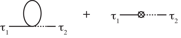
Evaluating Fig. 1 gives the following result for the 1-loop correction [3, 5, 6]

$$G_{\scriptscriptstyle C}^{1}(k,\tau_{1},\tau_{2})=-\frac{\lambda}{2}\int_{-\infty}^{0}{\rm d}\tau^{\prime}a^{4}(\tau^{\prime})\,G_{\scriptscriptstyle C}^{0}(k,\tau_{1},\tau^{\prime})\,G_{\scriptscriptstyle R}^{0}(k,\tau^{\prime},\tau_{2})\,\Lambda(\tau^{\prime})+(\tau_{1}\leftrightarrow\tau_{2})$$ (20)

where the factor of $\frac{1}{2}$ is from the combinatorics of the contractions, and the quantity $\Lambda(\tau)$ is the momentum integral given by Eq. (2.2). The contribution coming from long-wavelength, super-Hubble modes is obtained by specializing to that part of the integration region for which we can use the asymptotic form for $-k\tau_{1,2}\ll 1$. Dropping ${\cal O}(1)$ terms relative to $\ln(-k\tau)$ gives

$$G_{\scriptscriptstyle C}^{1}(k,\tau_{1},\tau_{2}) \simeq -\frac{\lambda}{2}\left(\frac{H}{2\pi}\right)^{2}\frac{1}{6k^{3}}\int_{-1/k}^{\tau_{1}}\frac{{\rm d}\tau^{\prime}}{\tau^{\prime}}\left[\left(\frac{\tau_{1}}{\tau^{\prime}}\right)^{3}-1\right]\,\ln\left(\frac{\mu}{\Lambda_{{\scriptscriptstyle I\kern-0.50003ptR}}}\right)+(\tau_{1}\leftrightarrow\tau_{2})$$ (21)

$$\simeq \frac{\lambda}{2}\left(\frac{H}{2\pi}\right)^{2}\frac{1}{6k^{3}}\,\ln\left(\frac{\mu}{\Lambda_{{\scriptscriptstyle I\kern-0.50003ptR}}}\right)\,[\ln(-k\tau_{1})+\ln(-k\tau_{2})]+\cdots\,.$$

Finally, evaluating at equal times, $\tau_{1}=\tau_{2}\equiv\tau$, gives the following, IR-divergent, next-to-leading contribution to $G_{\scriptscriptstyle C}$:

$$G_{\scriptscriptstyle C}(k,\tau)=\frac{H^{2}}{2k^{3}}\left[1+\frac{\lambda}{3(2\pi)^{2}}\ln\left(\frac{\mu}{\Lambda_{\scriptscriptstyle I\kern-0.50003ptR}}\right)\ln\left(-k\tau\right)+\cdots\right]\,,$$ (22)

coming from super-Hubble modes. Here the ellipses denote terms whose contributions do not diverge as either $\Lambda_{\scriptscriptstyle I\kern-0.50003ptR}$ or $-k\tau$ vanish, and so are subdominant to those explicitly displayed.

2.4 Large logs and secular time dependence

Eq. (22) displays two separate kinds of large logarithms. The one of interest for the arguments of the next section is the $\ln(-k\tau)$ term, since this displays the secular time-dependence for which the dynamical renormalization group is designed. This term is proportional to the number of $e$-folds between horizon exit of the mode $k$ and the time $\tau$ where we evaluate the result: $-k\tau=k/(aH)=a_{k}/a$. For calculations of curvature perturbations resulting from inflation, this apparent growth does not give rise to a physical divergence: the curvature perturbation is conserved outside the horizon and in fact one may follow the classical evolution of the modes shortly after horizon crossing until horizon re-entry [23].

The other large log is the IR divergence as $\Lambda_{\scriptscriptstyle I\kern-0.50003ptR}\to 0$. This has its origin both in the use of massless fields, and in the eternity of de Sitter space that the above calculation implicitly assumes holds in the past of $\tau$. As discussed earlier, this divergence ultimately cancels some other dependence on $\Lambda_{\scriptscriptstyle I\kern-0.50003ptR}$ in a physical observable, and because the divergence is logarithmic the cancellation of $\Lambda_{\scriptscriptstyle I\kern-0.50003ptR}$ gives

$$G_{\scriptscriptstyle C}(k,\tau)=\frac{H^{2}}{2k^{3}}\left[1+\frac{\lambda}{3(2\pi)^{2}}\ln\left(\mu L\right)\ln\left(-k\tau\right)+\cdots\right]\,,$$ (23)

where $L$ is a physical scale associated with whatever long-distance physics makes the result IR finite. The precise nature of this scale is model-dependent, because it cannot be identified purely within the UV part of the theory we use to this point. We identify below what $L$ is in the specific case where it is a mass that provides the convergence.

3 RG Methods

This section briefly recaps standard lowest-order RG arguments, for their later use in our cosmological applications. Part of our purpose is also to emphasize how the use of the RG equations avoids the necessity of performing explicit summations over infinite classes of graphs.

3.1 The standard argument

Standard one-loop calculations for dimensionless couplings give the value of the renormalized couplings, $\alpha(\mu)$, for different values of the renormalization point, $\mu$:

$$\alpha(\mu)=\alpha(\mu_{0})+b\,\alpha^{2}(\mu_{0})\,\ln\left(\frac{\mu}{\mu_{0}}\right)\,,$$ (24)

where $b$ is a calculable number. The domain of validity of this calculation requires both $\alpha(\mu_{0})\ll 1$ and $\alpha(\mu_{0})\ln(\mu/\mu_{0})\ll 1$.

The RG proceeds [29] by differentiating the above result with respect to $\mu$, giving

$$\mu\,\frac{\partial\alpha}{\partial\mu}=b\,\alpha^{2}\,,$$ (25)

where, to within the accuracy given, $\alpha$ on both sides can be taken to be $\alpha(\mu)$. This equation can be integrated to give the solution

$$\frac{1}{\alpha(\mu)}=\frac{1}{\alpha(\mu_{0})}-b\,\ln\left(\frac{\mu}{\mu_{0}}\right)\,.$$ (26)

The point of this seemingly content-free exercise of differentiating and then integrating the loop result is this: while eq. (24) relies on the product $\alpha\ln(\mu/\mu_{0})$ being small, eqs. (25) and (26) only require $\alpha$ be small and so have a larger domain of validity, applying in particular when $\alpha\ln(\mu/\mu_{0})$ is order unity. Integrating the RG equation effectively resums the leading logs. Notice that this resummation selectively takes terms to all orders in $\alpha\ln(\mu/\mu_{0})$, but this does not rely on identifying which subclass of graphs is dominant.

3.2 The dynamical RG

The dynamical RG [19] uses a similar logic to identify the long-time behavior of solutions when perturbative methods generate perturbations that grow secularly with time. For instance, suppose an approximation scheme based on expanding in a small parameter $\varepsilon$ produces a result of the form

$$y(t) = y_{0}(t)+\varepsilon\,y_{1}(t)+{\cal O}\left(\varepsilon^{2}\right)$$ (27)

$$= y_{0}(c,t)+\varepsilon\,y_{1}(c,t)+{\cal O}\left(\varepsilon^{2}\right)\,,$$

where the second line emphasizes the dependence of the solution at each order in $\varepsilon$ on the integration constant, $c$, of $y_{0}(t)$. Of particular interest is when $y_{1}(t)$ is a secular, growing function of time. When this is so, the expansion in powers of $\varepsilon$ breaks down for time-scales, $t>T$, where $\varepsilon y_{1}(T)/y_{0}(T)$ is order unity.

The dynamical RG shows how to infer the behavior of the solution for times $t>T$. To do so, first introduce an arbitrary time scale, $\vartheta$, with

$$y(t)=y_{0}(t)+\varepsilon\,\Bigl{[}y_{1}(t)-y_{1}(\vartheta)+y_{1}(\vartheta)\Bigr{]}+{\cal O}\left(\varepsilon^{2}\right)\,,$$ (28)

and absorb the last $y_{1}(\vartheta)$ term into the zeroeth-order integration constants:

$$y_{0}[c(\vartheta),t]:=y_{0}(c,t)+\varepsilon\,y_{1}(\vartheta)\,,$$ (29)

and so

$$y(t)=y_{0}[c(\vartheta),t]+\varepsilon\,\Bigl{[}y_{1}(t)-y_{1}(\vartheta)\Bigr{]}+{\cal O}\left(\varepsilon^{2}\right)\,.$$ (30)

The dynamical RG argument proceeds from the recognition that $y(t)$ is independent of $\vartheta$: ${\rm d}y/{\rm d}\vartheta=0$. Differentiating and dropping ${\cal O}(\varepsilon^{2})$ terms then gives

$$\left(\frac{\partial y_{0}}{\partial c}\right)\,\frac{{\rm d}c}{{\rm d}\vartheta}-\varepsilon\,\frac{\partial y_{1}(c,\vartheta)}{\partial\vartheta}=0\,,$$ (31)

which can be regarded as a differential equation to be solved for $c(\vartheta)$, whose solution is $c=\tilde{c}(\vartheta)$.

The argument is now the usual one: the solution $c=\tilde{c}(\vartheta)$ has a broader domain of validity (typically simply $\varepsilon\ll 1$) than does the initial definition of $c(\vartheta)$ (which required $\varepsilon\,y_{1}(t)\ll 1$). The final late-time behavior is then found by using the fact that $y(t)$ does not depend on $\vartheta$ to make the convenient choice $\vartheta=t$, and so

$$y(t) = y_{0}[\tilde{c}(\vartheta),t]+\varepsilon\,\Bigl{[}y_{1}(t)-y_{1}(\vartheta)\Bigr{]}+{\cal O}\left(\varepsilon^{2}\right)$$ (32)

$$= y_{0}[\tilde{c}(t),t]+{\cal O}\left(\varepsilon^{2}\right)\,.$$

This result resums the leading large-time behavior beyond the leading order perturbative result. Particularly simple is the case where

$$y(t)=c\,\left[1+\varepsilon\,f(t)+{\cal O}\left(\varepsilon^{2}\right)\right]\,,$$ (33)

where $y_{0}=c$ is time-independent. In this case $c(\vartheta)=c\,[1+\varepsilon\,f(\vartheta)]$ and so the condition ${\rm d}y/{\rm d}\vartheta=0$ implies

$$\frac{{\rm d}c}{{\rm d}\vartheta}-\varepsilon\,c\,\frac{{\rm d}f}{{\rm d}\vartheta}=0\,,$$ (34)

which integrates to give $c=\tilde{c}(\vartheta)$, where $\tilde{c}(\vartheta)=c\,e^{\varepsilon f(\vartheta)}$. This gives the resummed large-time solution

$$y(t)=c\,e^{\varepsilon f(t)}\left[1+{\cal O}\left(\varepsilon^{2}\right)\right]\,.$$ (35)

This is the particular case that arises in the one-loop scalar calculation on de Sitter space.

3.3 The dynamical RG for de Sitter fluctuations

Earlier sections show the leading infrared-sensitive part of the de Sitter space calculation of massless-scalar fluctuations involves a secular time dependence,

$$G_{\scriptscriptstyle C}(k,\tau)=\frac{H^{2}}{2k^{3}}\left[1+\frac{\lambda}{3(2\pi)^{2}}\ln\left(\mu L\right)\ln\left(-k\tau\right)+\cdots\right]\,,$$ (36)

with ellipses indicating terms that do not diverge when $L$ or $-k\tau$ vanish. For this result, and assuming that the scale $L$ is independent of $t$ — as is the case if the IR physics is de Sitter invariant (like a scalar mass term) — the dynamical RG resummation described above predicts the following long-time behavior

$$G_{\scriptscriptstyle C}(k,\tau) = \frac{H^{2}}{2k^{3}}\exp\left[+\frac{\lambda}{3(2\pi)^{2}}\ln\left(\mu L\right)\ln\left(-k\tau\right)\right]\Bigl{(}1+\cdots\Bigr{)}$$ (37)

$$= \frac{H^{2}}{2k^{3}}\left(\frac{k}{aH}\right)^{\delta}\Bigl{(}1+\mathcal{O}(\delta^{2})\Bigr{)}\,,$$

with

$$\delta=\frac{\lambda}{3(2\pi)^{2}}\ln\left(\mu L\right)\,.$$ (38)

This resummed result holds to all orders in $\delta\ln(-k\tau)$, but neglects terms that are suppressed by additional powers of $\delta$ without accompanying powers of $\ln(-k\tau)$. Its validity therefore requires $\delta\ll 1$, although this condition might also be relaxed through an RG resummation of the large $\ln\left(\mu L\right)$ logarithm.

Notice that because $\mu L\gg 1$ and $\lambda>0$ the power $\delta$ is also positive, implying that the DRG-improved correlator, eq. (37), is less singular as $k\to 0$ than is the zeroth-order result, $G^{0}_{\scriptscriptstyle C}(k,\tau)\propto H^{2}/k^{3}$. Also notice that although we do not need to know which subclass of graphs is dominant in making this argument, the results of ref. [6] show that these leading logs come from the ‘chain’ diagrams that repeatedly insert a scalar self-energy. The validity of the DRG does not require that these entire diagrams dominate all of the others, but only that they dominate in their contribution to the leading logs.

4 Comparisons to other results

This section makes three points. First, the small-$k$ limit of the above DRG expression for $G_{\scriptscriptstyle C}(k,\tau)$ is argued to be similar to the small-$k$ result for a massive scalar, showing that the resummed late-time behavior softens the IR divergence in way very similar to a mass. Second, the super-Hubble part of the loop calculation is repeated using massive scalars, to show precisely what the large logarithm $\ln(\mu L)$ means in an explicit example for which the IR physics is known and calculable. Finally, we extend our calculations to an $N$-scalar model for which a dynamical mass is known to be generated within a controllable approximation in the large-$N$ limit. We do so in order to show more precisely how the DRG resummation reproduces the effects of the dynamically resummed mass.

4.1 Massive scalar field

A massive scalar field in de Sitter space provides the simplest example of IR-convergent, de Sitter invariant, physics which nonetheless can have interesting contributions from super-Hubble modes if the mass is less than the Hubble scale. Just as is true for flat space, a mass term improves the IR convergence by making propagators less singular for small $k$. To see why this is so for de Sitter space, recall that the massive scalar propagator obtained from the general mode functions, eq.(9), becomes, in the limit $-k\tau=k/(aH)\ll 1$

$$G_{\scriptscriptstyle C}^{0}(k,\tau_{1},\tau_{2}) \simeq \frac{H^{2}}{2k^{3}}(k^{2}\tau_{1}\tau_{2})^{\epsilon}$$ (39)

$$G_{\scriptscriptstyle R}^{0}(k,\tau_{1},\tau_{2}) \simeq \theta(\tau_{1}-\tau_{2})\frac{H^{2}}{3}(\tau_{1}^{3-\epsilon}\tau_{2}^{\epsilon}-\tau_{1}^{\epsilon}\tau_{2}^{3-\epsilon})\,.$$ (40)

where $\epsilon={M^{2}}/{3H^{2}}$. As advertised, these expressions cure the IR divergences encountered previously because they are less singular than the massless case as $k\to 0$. But for $M^{2}\ll H^{2}$ the growth of the difference between the massive and massless expressions for $G_{\scriptscriptstyle C}(k,\tau)$ is much slower than in flat space, with significant deviations only arising once $(-k\tau)^{2\epsilon}$ deviates from unity. This occurs for $k<k_{*}$ with

$$-k_{*}\tau=\frac{k_{*}}{aH}\simeq e^{-1/2\epsilon}=e^{-3H^{2}/2M^{2}}\,,$$ (41)

and so $k_{*}/a\simeq H\,e^{-3H^{2}/2M^{2}}$ can be much smaller than $M$.

What is important for the present purposes is that the small-$k$ form of the massive propagator has the same kind of $k$-dependence as does the DRG-resummed result for the massless field: both behave as $G_{\scriptscriptstyle C}\propto k^{\alpha-3}$, for $\alpha>0$. For massive particles we have $\alpha=2\epsilon=2M^{2}/3H^{2}$ while DRG resummation gives $\alpha=\lambda\ln(\mu L)/12\pi^{2}$. Equating these powers shows that the DRG-resummed long-wavelength correlator behaves as if it describes a dynamically generated mass of order

$$M^{2}_{\rm eff}\simeq\frac{\lambda H^{2}}{8\pi^{2}}\,\ln(\mu L)\,.$$ (42)

A reasonable guess for the size to take for $L$ in this expression is

$$L\simeq\frac{a}{k_{*}}\simeq\frac{1}{H}\;e^{1/2\epsilon}\,,$$ (43)

(a more precise choice for $L$ is described shortly), in which case we have

$$M^{2}_{\rm eff}\simeq\frac{\lambda H^{2}}{8\pi^{2}}\,\ln\left(\frac{\mu}{H}\right)+\frac{3\lambda H^{4}}{16\pi^{2}M^{2}}\,.$$ (44)

4.2 Massive loop calculation

It is instructive to repeat the IR-sensitive, super-Hubble part of the loop calculation using this same massive scalar (still with a quartic self-interaction), since this provides a simple and specific example of IR-safe physics that can cure the IR divergences of the massless case. Among other things, such a calculation allows us to identify more precisely what the large logarithm $\ln(\mu L)$ means when it is a small mass that is responsible for IR convergence.

So far as the purpose of identifying the IR behavior is concerned, what is important is following the contribution of the super-Hubble modes in the result. For the loop factor, $\Lambda(\tau)$, the contribution of these modes is

$$\Lambda(\tau) \simeq \frac{H^{2}}{(2\pi)^{2}}\int_{a\,\Lambda_{{\scriptscriptstyle I\kern-0.50003ptR}}}^{a\,\Lambda_{\scriptscriptstyle U\kern-0.50003ptV}}\frac{{\rm d}p}{p}\left(-p\,\tau\right)^{2\epsilon}+\hbox{c.t.}\simeq\frac{H^{2}}{(2\pi)^{2}}\int_{a\,\Lambda_{{\scriptscriptstyle I\kern-0.50003ptR}}}^{a\,\mu}\frac{{\rm d}p}{p}\;\left(-p\,\tau\right)^{2\epsilon}$$ (45)

$$\simeq \frac{1}{2\epsilon}\left(\frac{H}{2\pi}\right)^{2}\left[\left(\frac{\mu}{H}\right)^{2\epsilon}-\left(\frac{\Lambda_{\scriptscriptstyle I\kern-0.50003ptR}}{H}\right)^{2\epsilon}\right]\,,$$

which is again $\tau$-independent because of the choice that $\Lambda_{\scriptscriptstyle I\kern-0.50003ptR}$ and $\mu$ are physical scales. Notice that in the limit $\epsilon\to 0$ eq. (45) approaches the super-Hubble part of the massless case, eq. (2.2),

$$\lim_{\epsilon\to 0}\Lambda=\left(\frac{H}{2\pi}\right)^{2}\ln\left(\frac{\mu}{\Lambda_{\scriptscriptstyle I\kern-0.50003ptR}}\right)\,,$$ (46)

but instead converges in the IR if $\epsilon$ is held fixed:

$$\lim_{\Lambda_{\scriptscriptstyle I\kern-0.50003ptR}\to 0}\Lambda=\frac{1}{2\epsilon}\left(\frac{H}{2\pi}\right)^{2}\left(\frac{\mu}{H}\right)^{2\epsilon}\,.$$ (47)

Here $\mu$ is, as before, a renormalization scale associated with the UV counterterms. Using eq. (47) to evaluate the 1-loop result, Fig. 1, then gives

$$G_{\scriptscriptstyle C}^{1}(k,\tau_{1},\tau_{2}) = -\frac{\lambda}{2}\int{\rm d}\tau^{\prime}a^{4}(\tau^{\prime})\,G_{\scriptscriptstyle C}^{0}(k,\tau_{1},\tau^{\prime})\,G_{\scriptscriptstyle R}^{0}(k,\tau^{\prime},\tau_{2})\,\Lambda(\tau^{\prime})+(\tau_{1}\leftrightarrow\tau_{2})$$ (48)

$$= -\frac{\lambda}{2}\left[\frac{1}{2\epsilon}\left(\frac{H}{2\pi}\right)^{2}\left(\frac{\mu}{H}\right)^{2\epsilon}\right]\frac{1}{6k^{3}}\int_{-1/k}^{\tau_{1}}\frac{{\rm d}\tau^{\prime}}{\tau^{\prime}}\;\left[\left(\frac{\tau_{1}}{\tau^{\prime}}\right)^{3-\epsilon}-\left(\frac{\tau_{1}}{\tau^{\prime}}\right)^{\epsilon}\right](k^{2}\tau^{\prime}\tau_{2})^{\epsilon}$$

$$\qquad\qquad\qquad\qquad\qquad\qquad\qquad\qquad\qquad\qquad+(\tau_{1}\leftrightarrow\tau_{2})$$

$$\simeq \frac{\lambda}{4\epsilon}\left(\frac{H}{2\pi}\right)^{2}\frac{1}{6k^{3}}\left(\frac{k^{2}\mu^{2}\tau_{1}\tau_{2}}{H^{2}}\right)^{\epsilon}\left[\ln\left(-k\tau_{1}\right)+\ln\left(-k\tau_{2}\right)+\cdots\right]\,,$$

where the unwritten terms are finite as $k\tau\to 0$. We find in this way the loop-corrected result

$$G_{\scriptscriptstyle C}(k,\tau)\simeq\frac{H^{2}}{2k^{3}}(-k\tau)^{2\epsilon}\left[1+\frac{\lambda}{6(2\pi)^{2}\epsilon}\,\left(\frac{\mu}{H}\right)^{2\epsilon}\ln(-k\tau)+\cdots\right]\,.$$ (49)

Notice that this is similar to expression (36) in the massless case, with the replacement

$$\ln(\mu L)\to\frac{1}{2\epsilon}\left(\frac{\mu}{H}\right)^{2\epsilon}=\frac{3H^{2}}{2M^{2}}\,\left(\frac{\mu}{H}\right)^{3M^{2}/3H^{2}}\,.$$ (50)

For small $\epsilon$ this reduces to

$$\ln(\mu L)\simeq\frac{1}{2\epsilon}+\ln\left(\frac{\mu}{H}\right)+{\cal O}(\epsilon^{2})\,,$$ (51)

which agrees with the simpler estimate, eq. (43), of the previous section. In this case the large logarithm $\ln(\mu L)$ is seen to correspond in the full result to the enhancement of the loop contribution by the factor $1/\epsilon$.

DRG resummation

Applying the DRG to resum the leading logs gives in this case the late-time result

$$G_{\scriptscriptstyle C}(k,\tau)\simeq\frac{H^{2}}{2k^{3}}(-k\tau)^{2\epsilon+\delta_{m}}$$ (52)

where

$$\delta_{m}=\frac{\lambda}{6(2\pi)^{2}\epsilon}\left(\frac{\mu}{H}\right)^{2\epsilon}\,,$$ (53)

confirming that the resummed leading logs modify $G_{\scriptscriptstyle C}(k,\tau)$ in the same way as would a mass. Notice that although this resums terms to all order in $\delta_{m}\ln(-k\tau)$, it requires $\delta_{m}\ll 1$, and so breaks down once $\lambda/\epsilon$ becomes too small. When both masses and couplings are present the mass effect dominates the coupling effect so long as $\delta_{m}<2\epsilon$, or

$$\frac{\lambda}{(4\pi)^{2}}<3\epsilon^{2}\left(\frac{H}{\mu}\right)^{2\epsilon}=\frac{M^{4}}{3H^{4}}\left(\frac{H}{\mu}\right)^{2M^{2}/3H^{2}}\,.$$ (54)

For $\lambda$ larger than this it is the coupling that dominates in the IR, and it contributes in the same way as would a mass of order

$$M^{2}_{\rm eff}=\frac{3H^{2}}{2}\;\delta_{m}=\frac{\lambda H^{2}}{(4\pi)^{2}\epsilon}\left(\frac{\mu}{H}\right)^{2\epsilon}\simeq\frac{3\lambda H^{4}}{(4\pi)^{2}M^{2}}\,,$$ (55)

where the last approximation neglects corrections that are of order $\epsilon$, since the assumption that the coupling effect dominates requires $\epsilon^{2}$ to be systematically small relative to $\lambda/(4\pi)^{2}$.

Notice that eq. (55) precisely agrees with what would be expected in a mean-field approximation, for which $M^{2}_{mf}\simeq\frac{1}{2}\,\lambda\langle\phi^{2}\rangle$, given the nonzero expectation

$$\langle\phi^{2}\rangle\simeq\frac{3H^{4}}{8\pi^{2}M^{2}}\,,$$ (56)

that a massive scalar field prepared in the Bunch-Davies vacuum acquires in de Sitter space [34, 35]. To this extent the DRG-improved long-time limit agrees with what would be expected from a stochastic approach [21] to super-Hubble scalar fluctuations. We explore this in more detail using a large-$N$ limit [21, 10, 6] in the next section.

4.3 Dynamical mass at large $N$

Large-$N$ expansions provide a useful laboratory for understanding dynamical resummations within a controlled approximation, and so we therefore pause to examine them briefly here. In this section we apply the dynamical RG to the large-$N$ generalization of the above calculation in order to show how it compares with the long-time behavior predicted by the DRG.

Consider to this end the large-$N$ generalization of our model,

$$S = -\int{\rm d}^{4}x\;\sqrt{-g}\;\left[\frac{1}{2}\,g^{\mu\nu}\,\partial_{\mu}\Phi^{\scriptscriptstyle T}\,\partial_{\nu}\Phi+V_{0}+\frac{1}{2}\Bigl{(}m^{2}+\xi R\Bigr{)}\,(\Phi^{\scriptscriptstyle T}\Phi)+\frac{\lambda}{4!}\,(\Phi^{\scriptscriptstyle T}\Phi)^{2}\right]$$

$$= -\int{\rm d}^{4}x\;\sqrt{-g}\;\left[\frac{1}{2}\,g^{\mu\nu}\,\partial_{\mu}\Phi^{\scriptscriptstyle T}\,\partial_{\nu}\Phi+V_{0}+\frac{M^{2}}{2}\,(\Phi^{\scriptscriptstyle T}\Phi)-\frac{\lambda}{4!}\left(s^{2}-2s\,\Phi^{\scriptscriptstyle T}\Phi\right)\right]\,,$$

where $M^{2}=m^{2}-12\,\xi H^{2}$ in de Sitter space, $\Phi$ denotes an $N$-component column vector of real scalar fields, and the first line follows from the second if $s$ is integrated out using the exact result

$$s=\Phi^{\scriptscriptstyle T}\Phi\,.$$ (58)

The scalar field equation for $\Phi$ in this model is

$$-\Box\Phi+\left(M^{2}+\frac{\lambda s}{6}\right)\,\Phi=0\,.$$ (59)

In the limit of large $N$ we take $\lambda$ small and $\langle s\rangle$ large, so that $g=N\lambda$ and $\sigma=\langle s\rangle/N$ are fixed. In this large-$N$ limit the field equation behaves sensibly, taking the mean-field form [36]

$$-\Box\Phi+\left[M^{2}+\frac{g\sigma}{6}\right]\,\Phi=0\,,$$ (60)

which uses the large-$N$ expression $\lambda s\,\Phi=g\sigma\,\Phi\left(1+2/N\right)+\cdots$. This shows that the scalar self-interaction contributes to the mass for $\Phi$ in the large-$N$ limit when terms of order $1/N$ are dropped

$$M^{2}_{\scriptscriptstyle N}=M^{2}+\frac{g\sigma}{6}=m^{2}-12\,\xi H^{2}+\frac{g\sigma}{6}\,,$$ (61)

provided only that $\sigma$ is nonzero.

The static value for $\sigma$ can also be computed for large $N$ in de Sitter space, with a standard result given by the contribution of $N$ free scalar fields [34, 35]:

$$\sigma=\frac{1}{N}\,\langle\Phi^{\scriptscriptstyle T}\Phi\rangle=\frac{3H^{4}}{8\pi^{2}M^{2}}\,,$$ (62)

and so

$$M^{2}_{{\scriptscriptstyle N}}=M^{2}+\frac{g\sigma}{6}=M^{2}+\frac{gH^{4}}{(4\pi)^{2}M^{2}}\,.$$ (63)

Using this mean-field mass in the $\Phi_{\scriptscriptstyle C}$ correlator then gives the large-$N$ expectation for the form of the small-$k$ limit of the de Sitter correlator

$$G_{\scriptscriptstyle C}(k,\tau)\simeq\frac{H^{2}}{2k^{3}}(-k\tau)^{2\epsilon_{{\scriptscriptstyle N}}}\,,$$ (64)

where

$$2\epsilon_{{\scriptscriptstyle N}}=\frac{2M^{2}_{{\scriptscriptstyle N}}}{3H^{2}}=\frac{2M^{2}}{3H^{2}}+\frac{gH^{2}}{6(2\pi)^{2}M^{2}}\,.$$ (65)

DRG resummation

For comparison we instead compute $G_{\scriptscriptstyle C}(k,\tau)$ perturbatively in $g$, and repeat the loop calculation of the previous section in the large-$N$ limit. There are only two changes required. One change comes from evaluating the combinatorial factors arising from performing the contractions of the various fields appearing in Fig. 1, which converts a factor of 3 (from counting the number of ways to contract fields) in the previous loop calculation into $(2+N)$. The second change is the replacement of the coupling, $\lambda\to g/N$, and so the generalization to arbitrary $N$ of the previously obtained loop result is obtained by making the simple replacement

$$3\lambda\to g\left(1+\frac{2}{N}\right)\,.$$ (66)

This leads to the following large-$N$ generalization of eq. (49),

$$G_{\scriptscriptstyle C}(k,\tau)\simeq\frac{H^{2}}{2k^{3}}(-k\tau)^{2\epsilon}\left[1+\frac{g}{18(2\pi)^{2}\epsilon}\,\left(\frac{\mu}{H}\right)^{2\epsilon}\ln(-k\tau)+\cdots\right]\,.$$ (67)

Using the DRG to resum the large-$\tau$ behavior gives, as before

$$G_{\scriptscriptstyle C}(k,\tau)\simeq\frac{H^{2}}{2k^{3}}(-k\tau)^{2\epsilon+\delta_{m}}\,,$$ (68)

where

$$\delta_{m}=\frac{g}{18(2\pi)^{2}\,\epsilon}\left(\frac{\mu}{H}\right)^{2\epsilon}\simeq\frac{gH^{2}}{6(2\pi)^{2}M^{2}}\,,$$ (69)

and the second, approximate, expression uses $\epsilon\ll 1$ to drop the factor $(\mu/H)^{2\epsilon}$ (compare with eq. (53)) . For small $k$ the total power of $k$ therefore is

$$2\epsilon+\delta_{m}=\frac{2M^{2}}{3H^{2}}+\frac{gH^{2}}{6(2\pi)^{2}M^{2}}\,,$$ (70)

in exact agreement with $\epsilon_{\scriptscriptstyle N}$ obtained using the large-$N$, mean-field result, eq. (65).

Self-consistent masses

The large-$N$ limit also allows a more careful exploration of the case of very small $M^{2}$. Because the dynamical mass, $M_{\scriptscriptstyle N}^{2}$ of eq. (63), is bounded from below, the physical mass does not disappear even in the limit $M^{2}\to 0$. Instead it reaches its minimum value when $\partial M_{\scriptscriptstyle N}^{2}/\partial M^{2}=0$, or

$$M^{2}_{\rm min}=\frac{1}{4\pi}\sqrt{g}\;H^{2}\,.$$ (71)

Because $g/\epsilon\simeq\sqrt{g}$ for this value of $M^{2}$ it lies within the domain of validity of our approximate expressions, which require $g/\epsilon\ll 1$. The subsequent growth of $M^{2}_{\scriptscriptstyle N}$ for smaller $M^{2}$ than this is suspect because $g/\epsilon$ becomes larger than unity. This means that eq. (71) corresponds to the smallest mass that it is possible to get within the domain of validity of our approximations. (The corresponding result for $N=1$ would be $M^{2}_{\rm min}=\sqrt{3\lambda}\;H^{2}/4\pi$. This mass is one that has been obtained by solving a ‘gap’ equation, in ref. [6], and agrees with the much earlier result of Starobinsky and Yokoyama [21], after rescaling to match their definition of $\lambda$.)

5 Scalar field with a cubic interaction

In this section we consider a slightly different case: a scalar field with a purely cubic interaction

$$V(\phi)=\frac{h}{3!}\,\phi^{3}\,,$$ (72)

with no mass term and no quartic interaction. We find in this case that the DRG-improved super-Hubble contributions do not have a momentum dependence appropriate to a dynamically generated mass.

$\begin{array}[]{ccc}\includegraphics[width=130.08731pt,angle={0}]{CubicA.pdf}&\includegraphics[width=130.08731pt,angle={0}]{CubicB.pdf}&\includegraphics[width=130.08731pt,angle={0}]{CubicC.pdf}\\ \mbox{(a)}&\mbox{(b)}&\mbox{(c)}\end{array}$

Figure 2: The three contributions to $G_{c}(k,\tau_{1},\tau_{2})$ at one loop. Diagram (a) is divergent in the UV and IR, (b) is only IR divergent, and (c) diverges only in the UV.

The one-loop graphs (other than the counterterms) contributing to $G_{\scriptscriptstyle C}(k,\tau_{1},\tau_{2})$ in this theory are shown in Figure 2. We evaluate these graphs using only the long-wavelength, super-Hubble limit of the propagators, as before. All graphs contribute a factor of $[\ln(-k\tau)]^{2}$ thanks to the two interaction vertices, but each has a different structure of divergences in the momentum integral. The first diagram gives a contribution that grows in time and is proportional to $\Lambda=(H/2\pi)^{2}\ln(\mu/\Lambda_{\scriptscriptstyle I\kern-0.50003ptR})$, as in the $\phi^{4}$ case. The second diagram converges in the UV and the momentum integral is dominated by loop momenta $p\gg k$. The last graph is UV divergent but not IR singular, and so does not contribute to the terms of present interest.

Evaluating the contribution of the first and second graphs gives the equal-time result

$$G_{\scriptscriptstyle C}(k,\tau,\tau) = G_{\scriptscriptstyle C}^{0}(k,\tau,\tau)\left\{1+\frac{h^{2}}{9H^{4}}\left[\ln^{2}(-k\tau)+\frac{4}{3}\ln(-k\tau)\right.\right.$$

$$\left.\left.\qquad\qquad\qquad+\frac{2}{3}(-k\tau)^{3}\ln(-k\tau)+\frac{2}{9}\right]\left[4\Lambda+\frac{H^{2}}{(2\pi)^{2}}\ln\left(\frac{k}{a\Lambda_{IR}}\right)\right]\right\}$$

$$= G_{\scriptscriptstyle C}^{0}(k,\tau,\tau)\left\{1+\frac{h^{2}}{9(2\pi)^{2}H^{2}}\ln^{3}(-k\tau)+\frac{4h^{2}\Lambda}{9H^{4}}\ln^{2}(-k\tau)+\dots\right\}\,,$$

where $\Lambda(\tau)=(H/2\pi)^{2}\ln(\mu/\Lambda_{\scriptscriptstyle I\kern-0.50003ptR})$ is as defined in the previous section, and the second line uses $k/(a\,\Lambda_{IR})=(-k\tau)(H/\Lambda_{IR})$. A massive scalar field with a cubic interaction is treated in detail in [5], who also do a careful analysis of the UV pieces. However, the IR part of the calculation above is sufficient to contrast the result of the DRG for this case with the quartic interaction result.

Applying the DRG method to this expression exponentiates the quantity in parenthesis,

$$G_{\scriptscriptstyle C}(k,\tau,\tau) = G_{\scriptscriptstyle C}^{0}(k,\tau,\tau)\exp\left\{\frac{h^{2}}{9H^{2}}\left[\frac{1}{(2\pi)^{2}}\ln^{3}(-k\tau)+\frac{4\Lambda}{H^{2}}\ln^{2}(-k\tau)+\dots\right]\right\}\,,$$

which clearly does not share the small-$k$ dependence appropriate to a constant mass. This agrees with naive expectations, since even if a mean-field treatment were valid it would predict $M^{2}_{\rm dyn}\propto h\langle\phi\rangle=0$. But unlike the quartic case, for the purely cubic theory the semiclassical expansion about the solution $\langle\phi\rangle=0$ is unstable, making the study of its fluctuations problematic.

6 Conclusions

Loop calculations involving massless scalars in de Sitter space have long been known to be plagued by strong infrared effects. These arise due to the indefinite growth of fluctuations on super-Hubble scales. These long-wavelength effects complicate the precision calculation of inflationary observables, by potentially putting the late-time behavior beyond the reach of perturbative calculations.

We argue here that the DRG is a natural tool to use for this kind of problem, where secular time dependence limits the domain of validity of a perturbation expansion. It provides a simple way to resum these terms, thus allowing the late-time behavior to be extracted from perturbative calculations.

We apply the DRG to several simple examples, such as a single quartically self-coupled field as well as a large $N$ quartically coupled model. In these situations the resummed IR behavior is less singular than is the leading-order result, in a way that mimics the presence of a nonzero mass. The same analysis for a cubic scalar theory demonstrates that the cubic interaction apparently does not self-regulate by generating a mass.

Fortified by these checks, we believe that DRG is likely to prove to be very useful for more detailed studies of other puzzling aspects of late-time, long wavelength de Sitter fluctuations.

Another direction to take this work might be to consider situations where there the important long-distance physics breaks de Sitter invariance. This could happen because inflation is not eternal, instead beginning at the end of a pre-inflationary phase [22], or perhaps if dS space should prove to be only metastable, with the BD vacuum ultimately decaying on large scales due to the inhomogeneous structure, perhaps coming from the formation of bubbles of some new phase. Whatever this source of dS symmetry breaking is, the two point function becomes a function of time and one may wonder whether a DRG analysis can still be useful.

An interesting application of this type would be to reproduce past discussions of such secular behaviour, such as that of ref. [37] which discusses large infrared logarithms in a time-dependent situation, and argues, following a proposal of Starobinsky and Yokoyama [21], that these may be resummed [38] using ideas from stochastic inflation. Investigations of this point, and how it relates to the DRG techniques discussed here, are in progress. Previous arguments about applying RG techniques for the case where the dS symmetry is broken can be found in [40].

Appendix A Renormalization

When renormalizing the one-loop UV divergences it is important to keep all of the interactions whose counter-terms can be required to cancel divergences at one loop. For an $O(N)$-invariant system of $N$ scalar fields the required terms are:

$$S = -\int{\rm d}^{4}x\;\sqrt{-g}\;\left[\frac{1}{2}\,g^{\mu\nu}\,\partial_{\mu}\Phi^{\scriptscriptstyle T}\,\partial_{\nu}\Phi+\frac{1}{2}(m^{2}+\xi\,R)(\Phi^{\scriptscriptstyle T}\Phi)+\frac{\lambda}{4!}\,(\Phi^{\scriptscriptstyle T}\Phi)^{2}\right.$$

$$\qquad\qquad\qquad\qquad\left.\phantom{\frac{1}{2}}+V_{0}+A\,R+B\,R_{\mu\nu\lambda\rho}R^{\mu\nu\lambda\rho}+C\,R_{\mu\nu}R^{\mu\nu}+D\,R^{2}+E\,\Box R\right]\,.$$

The coefficients of these terms contain divergent contributions, whose presence cancels all UV divergences that arise at one loop. The counterterm lagrangian consists of the same terms with $m^{2}\to\delta m^{2}$, $\xi\to\delta\xi$ and so on.

Working in dimensional regularization, a standard calculation [39] gives the divergent part of the one-loop effective action, $\Sigma_{\infty}$, generated by an arbitrary collection of fields. Assuming these fields have an action of generic form

$$S=-\frac{1}{2}\int{\rm d}^{4}x\sqrt{-g}\;\Phi^{\scriptscriptstyle T}(-\Box+X)\Phi\,,$$ (76)

one finds

$$\Sigma_{\infty}=\pm\frac{1}{2}\,\left(\frac{1}{4\pi}\right)^{n/2}\Gamma(2-n/2)\,\mu^{n-4}\int{\rm d}^{n}x\sqrt{-g}\;{\rm tr}\,a_{2}\,,$$ (77)

where the upper (lower) sign applies for boson (fermions), $n\to 4$ denotes the dimension of spacetime, $\mu$ is the arbitrary mass scale that arises in dimensional regularization, and $a_{2}$ is the second Gilkey/de Witt coefficient,

$$a_{2} = \frac{1}{360}\Bigl{(}2R_{\mu\nu\lambda\rho}R^{\mu\nu\lambda\rho}-2R_{\mu\nu}R^{\mu\nu}+5R^{2}-12\Box R\Bigr{)}$$ (78)

$$\qquad\qquad+\frac{1}{6}\,R\,X+\frac{1}{2}\,X^{2}-\frac{1}{6}\,\Box X+\frac{1}{12}Y_{\mu\nu}Y^{\mu\nu}\,.$$

Here $[D_{\mu},D_{\nu}]\Phi=Y_{\mu\nu}\Phi$ defines $Y_{\mu\nu}$, where $D_{\mu}$ is the covariant derivative appearing within $\Box\Phi=g^{\mu\nu}D_{\mu}D_{\nu}\Phi$.

Since gauge-neutral scalars are the case of present interest, we have $Y_{\mu\nu}=0$. Further specializing to the potential $V=\frac{1}{2}(m^{2}+\xi\,R)(\Phi^{\scriptscriptstyle T}\Phi)+\frac{1}{4!}\,\lambda(\Phi^{\scriptscriptstyle T}\Phi)^{2}$ then gives

$$X=m^{2}+\xi\,R+\frac{\lambda}{6}\,(\Phi^{\scriptscriptstyle T}\Phi)+\frac{\lambda}{3}\,\Phi\,\Phi^{\scriptscriptstyle T}\,,$$ (79)

and so

$${\rm tr}\,X=N(m^{2}+\xi\,R)+\frac{\lambda}{6}(\Phi^{\scriptscriptstyle T}\Phi)\left(N+2\right)\,,$$ (80)

and

$${\rm tr}\,X^{2}=N(m^{2}+\xi R)^{2}+\frac{\lambda}{3}\,(m^{2}+\xi R)(\Phi^{\scriptscriptstyle T}\Phi)\left(N+2\right)+\frac{\lambda^{2}}{36}(\Phi^{\scriptscriptstyle T}\Phi)^{2}\left(N+8\right)\,.$$ (81)

Using these in eq. (78) gives the result

$${\rm tr}\,a_{2} = \frac{N}{360}\Bigl{(}2R_{\mu\nu\lambda\rho}R^{\mu\nu\lambda\rho}-2R_{\mu\nu}R^{\mu\nu}+5R^{2}-12\Box R\Bigr{)}$$ (82)

$$\qquad\qquad+\frac{1}{6}\,R\;{\rm tr}\,X+\frac{1}{2}\;{\rm tr}\,X^{2}-\frac{1}{6}\;\Box\,{\rm tr}\,X$$

$$= \frac{N}{180}\Bigl{(}R_{\mu\nu\lambda\rho}R^{\mu\nu\lambda\rho}-R_{\mu\nu}R^{\mu\nu}\Bigr{)}+\frac{N}{2}\left(\xi+\frac{1}{6}\right)^{2}R^{2}-\frac{N}{6}\left(\xi+\frac{1}{5}\right)\Box R$$

$$\qquad\qquad+\frac{Nm^{4}}{2}+N\left(\xi+\frac{1}{6}\right)m^{2}R+\frac{\lambda}{6}(N+2)\,m^{2}(\Phi^{\scriptscriptstyle T}\Phi)$$

$$\qquad\qquad+\frac{\lambda}{6}(N+2)\left(\xi+\frac{1}{6}\right)R\,(\Phi^{\scriptscriptstyle T}\Phi)+\frac{\lambda^{2}}{72}(N+8)(\Phi^{\scriptscriptstyle T}\Phi)^{2}$$

$$\qquad\qquad-\frac{\lambda}{36}\,(N+2)\,\Box(\Phi^{\scriptscriptstyle T}\Phi)\,.$$

Using the above results to compute $\Sigma_{\infty}$, shows that the one-loop divergences are given by poles as $n\to 4$ of the form

$$\Sigma_{\infty}=-\left(\frac{1}{4\pi}\right)^{n/2}\left(\frac{\mu^{n-4}}{n-4}\right)\int{\rm d}^{n}x\sqrt{-g}\;{\rm tr}\,a_{2}\,.$$ (83)

These can be absorbed into minimal-subtraction (MS) counter-terms of the form

$$\Sigma_{ct}=\left(\frac{1}{4\pi}\right)^{2}\int{\rm d}^{4}x\sqrt{-g}\;\left[\frac{1}{n-4}-\frac{1}{2}\ln\left(\frac{m^{2}}{\mu^{2}}\right)\right]\,{\rm tr}\,a_{2}\,,$$ (84)

and the counter-terms in other renormalization schemes differ from these by finite renormalizations. Notice that for the counterterm action unitarity requires that all fields are evaluated at $n=4$.

Comparing this with the counter-term action and differentiating with respect to $\mu$ shows (in minimal subtraction) that the renormalized couplings satisfy the renormalization group equations

$$\mu\frac{\partial m^{2}}{\partial\mu}=\frac{\lambda\,m^{2}N}{48\pi^{2}}\left(1+\frac{2}{N}\right)\,,\quad \quad\mu\frac{\partial\xi}{\partial\mu}=\frac{\lambda\,N}{48\pi^{2}}\left(\xi+\frac{1}{6}\right)\left(1+\frac{2}{N}\right)$$

$$\mu\frac{\partial\lambda}{\partial\mu}=\frac{\lambda^{2}N}{48\pi^{2}}\left(1+\frac{8}{N}\right)\,,\quad \quad\mu\frac{\partial V_{0}}{\partial\mu}=\frac{m^{4}N}{32\pi^{2}}$$

$$\mu\frac{\partial A}{\partial\mu}=\frac{m^{2}N}{16\pi^{2}}\left(\xi+\frac{1}{6}\right)\,,\quad \quad\mu\frac{\partial B}{\partial\mu}=-\mu\frac{\partial C}{\partial\mu}=\frac{N}{2880\pi^{2}}$$

$$\mu\frac{\partial D}{\partial\mu}=\frac{N}{32\pi^{2}}\left(\xi+\frac{1}{6}\right)^{2}\,,\quad \quad\mu\frac{\partial E}{\partial\mu}=-\frac{N}{96\pi^{2}}\left(\xi+\frac{1}{5}\right)\,.$$ (85)

These may be integrated in the usual way. Write the first few of these equations as

$$\mu\,\frac{\partial\xi}{\partial\mu}=b_{1}\,\lambda\left(\xi+\frac{1}{6}\right)\,,\quad\mu\,\frac{\partial m^{2}}{\partial\mu}=b_{1}\,\lambda\,m^{2}\,,$$ (86)

and

$$\mu\,\frac{\partial\lambda}{\partial\mu}=b_{2}\,\lambda^{2}\,,$$ (87)

where

$$b_{1}=\frac{N}{48\pi^{2}}\left(1+\frac{2}{N}\right)\quad\hbox{and}\quad b_{2}=\frac{N}{48\pi^{2}}\left(1+\frac{8}{N}\right)\,.$$ (88)

The $\lambda$ equation integrates to give

$$\lambda(\mu)=\frac{\lambda_{0}}{1-b_{2}\,\lambda_{0}\,\ln(\mu/\mu_{0})}\,,$$ (89)

and the other two give

$$\frac{\xi(\mu)+1/6}{\xi_{0}+1/6}=\frac{m^{2}(\mu)}{m^{2}_{0}}=\left[\frac{\lambda(\mu)}{\lambda_{0}}\right]^{p}\,,$$ (90)

where

$$p=\frac{b_{1}}{b_{2}}=\frac{N+2}{N+8}=1-\frac{6}{N}+\cdots\,,$$ (91)

and so $1>p\geq\frac{1}{3}$, with the smallest value occurring when $N=1$.

In particular,

$$m^{2}-12\,\xi H^{2}=m^{2}_{0}\left(\frac{\lambda}{\lambda_{0}}\right)^{p}-12\left(\xi_{0}+\frac{1}{6}\right)\left(\frac{\lambda}{\lambda_{0}}\right)^{p}+2H^{2}\,.$$ (92)

Recalling that both $b_{2}$ and $p=b_{1}/b_{2}$ are positive, we know $\lambda$ is not asymptotically free, and so $\mu<\mu_{0}$ implies both $\lambda<\lambda_{0}$ and $(\lambda/\lambda_{0})^{p}<1$. Consequently as $\lambda$ flows to 0 and $\xi$ flows to $-\frac{1}{6}$ with falling $\mu$, the quantity $m^{2}-12\,\xi H^{2}$ instead flows to $2H^{2}>0$, ensuring $m^{2}\to 0$ is necessarily much smaller than $12\,|\xi|H^{2}\to 2H^{2}$.

The Riemann- and Ricci-squared coefficients are also easily integrated, giving

$$B=B_{0}+\frac{N}{2880\pi^{2}}\,\ln\left(\frac{\mu}{\mu_{0}}\right)\quad\hbox{and}\quad C=C_{0}-\frac{N}{2880\pi^{2}}\,\ln\left(\frac{\mu}{\mu_{0}}\right)\,.$$ (93)

Those for $A$, $V_{0}$ and $D$ require integrating the previous expressions for $m^{2}(\mu)$ and $\xi(\mu)$, with

$$A(\mu) = A_{0}+\frac{N}{16\pi^{2}}\int_{\mu_{0}}^{\mu}\frac{{\rm d}\mu^{\prime}}{\mu^{\prime}}\;m^{2}(\mu^{\prime})\left(\xi(\mu^{\prime})+\frac{1}{6}\right)$$

$$= A_{0}+\frac{Nm_{0}^{2}}{16\pi^{2}}\,\left(\xi_{0}+\frac{1}{6}\right)\int_{\mu_{0}}^{\mu}\frac{{\rm d}\mu^{\prime}}{\mu^{\prime}}\left[\frac{\lambda(\mu^{\prime})}{\lambda_{0}}\right]^{2p}$$

$$= A_{0}+\frac{Nm_{0}^{2}}{16\pi^{2}}\,\left(\xi_{0}+\frac{1}{6}\right)\int_{0}^{\ln(\mu/\mu_{0})}\frac{{\rm d}t}{(1-b_{2}\lambda_{0}\,t)^{2p}}$$

$$= A_{0}+\frac{Nm_{0}^{2}}{16\pi^{2}\lambda_{0}(2b_{1}-b_{2})}\,\left(\xi_{0}+\frac{1}{6}\right)\left\{\frac{1}{[1-b_{2}\lambda_{0}\,\ln(\mu/\mu_{0})]^{2p-1}}-1\right\}$$

$$V_{0}(\mu) = V_{0}(\mu_{0})+\frac{Nm_{0}^{4}}{32\pi^{2}}\int_{\mu_{0}}^{\mu}\frac{{\rm d}\mu^{\prime}}{\mu^{\prime}}\left[\frac{\lambda(\mu^{\prime})}{\lambda_{0}}\right]^{2p}$$

$$= V_{0}(\mu_{0})+\frac{Nm_{0}^{4}}{32\pi^{2}\lambda_{0}(2b_{1}-b_{2})}\left\{\frac{1}{[1-b_{2}\lambda_{0}\,\ln(\mu/\mu_{0})]^{2p-1}}-1\right\}$$

$$D(\mu) = D_{0}+\frac{N}{32\pi^{2}}\left(\xi_{0}+\frac{1}{6}\right)^{2}\int_{\mu_{0}}^{\mu}\frac{{\rm d}\mu^{\prime}}{\mu^{\prime}}\;\left[\frac{\lambda(\mu^{\prime})}{\lambda_{0}}\right]^{2p}$$

$$= D_{0}+\frac{N}{32\pi^{2}\lambda_{0}(2b_{1}-b_{2})}\left(\xi_{0}+\frac{1}{6}\right)^{2}\left\{\frac{1}{[1-b_{2}\lambda_{0}\,\ln(\mu/\mu_{0})]^{2p-1}}-1\right\}\,.$$

Running in the large-$N$ limit

When taking the large-$N$ limit we write $\lambda=g/N$ and may take $b_{1}=b_{2}=Nb$, up to subdominant terms in $1/N$, with

$$b=\frac{1}{48\pi^{2}}\,.$$ (95)

Because $b_{1}=b_{2}$ at large $N$ we also have $p=b_{1}/b_{2}=1$ in this limit. The first few RG equations in this limit then become

$$\mu\frac{\partial m^{2}}{\partial\mu}=b\,g\,m^{2}\,,\qquad\mu\frac{\partial\xi}{\partial\mu}=b\,g\left(\xi+\frac{1}{6}\right)\,,\qquad\mu\frac{\partial g}{\partial\mu}=b\,g^{2}\,,$$ (96)

and so on. These integrate to give

$$\frac{\xi(\mu)+1/6}{\xi_{0}+1/6}=\frac{m^{2}(\mu)}{m^{2}_{0}}=\frac{g(\mu)}{g_{0}}=\frac{1}{1-b_{2}\,g_{0}\,\ln(\mu/\mu_{0})}\,,$$ (97)

which show that $m^{2}$, $\xi+\frac{1}{6}$ and $g$ all renormalize in the same way, up to $1/N$ corrections. This implies that the relative size of all of the terms in expressions like (61),

$$M^{2}_{\scriptscriptstyle N} = m^{2}-12\,\xi H^{2}+\frac{g\sigma}{6}$$ (98)

$$= 2H^{2}+m^{2}-12\,\left(\xi+\frac{1}{6}\right)H^{2}+\frac{g\sigma}{6}\,,$$

do not change as $\mu$ scales, and $M^{2}$ and $M^{2}_{\scriptscriptstyle N}$ both approach $2H^{2}$ as $\mu\to 0$.

References

- [1] E. Komatsu et al. [WMAP Collaboration], “Five-Year Wilkinson Microwave Anisotropy Probe (WMAP) Observations:Cosmological Interpretation,” Astrophys. J. Suppl. 180 (2009) 330 [arXiv:0803.0547 [astro-ph]]; M. Tegmark et al. [SDSS Collaboration], “Cosmological parameters from SDSS and WMAP,” Phys. Rev. D 69 (2004) 103501 [arXiv:astro-ph/0310723].
- [2] V. F. Mukhanov and G. V. Chibisov, JETP Lett. 33, 532 (1981) [Pisma Zh. Eksp. Teor. Fiz. 33, 549 (1981)]; A. H. Guth and S. Y. Pi, Phys. Rev. Lett. 49, 1110 (1982); A. A. Starobinsky, Phys. Lett. B 117, 175 (1982); S. W. Hawking, Phys. Lett. B 115, 295 (1982); V. N. Lukash, Pisma Zh. Eksp. Teor. Fiz. 31, 631 (1980); Sov. Phys. JETP 52, 807 (1980) [Zh. Eksp. Teor. Fiz. 79, (1980)]; W. Press, Phys. Scr. 21, 702 (1980); K. Sato, Mon. Not. Roy. Astron. Soc. 195, 467 (1981).
- [3] M. S. Sloth, “On the one loop corrections to inflation and the CMB anisotropies,” Nucl. Phys. B 748, 149 (2006) [arXiv:astro-ph/0604488]; “On the one loop corrections to inflation. II: The consistency relation,” Nucl. Phys. B 775, 78 (2007) [arXiv:hep-th/0612138].
- [4] A. Bilandzic and T. Prokopec, “Quantum radiative corrections to slow-roll inflation,” Phys. Rev. D 76, 103507 (2007) [arXiv:0704.1905 [astro-ph]].
- [5] M. van der Meulen and J. Smit, “Classical approximation to quantum cosmological correlations,” JCAP 0711, 023 (2007) [arXiv:0707.0842 [hep-th]].
- [6] G. Petri, “A Diagrammatic Approach to Scalar Field Correlators during Inflation,” arXiv:0810.3330 [gr-qc].
- [7] D. H. Lyth, “The curvature perturbation in a box,” JCAP 0712, 016 (2007) [arXiv:0707.0361 [astro-ph]].
- [8] K. Enqvist, S. Nurmi, D. Podolsky and G. I. Rigopoulos, “On the divergences of inflationary superhorizon perturbations,” JCAP 0804, 025 (2008) [arXiv:0802.0395 [astro-ph]].
- [9] N. Bartolo, S. Matarrese, M. Pietroni, A. Riotto and D. Seery, “On the Physical Significance of Infra-red Corrections to Inflationary Observables,” JCAP 0801, 015 (2008) [arXiv:0711.4263 [astro-ph]].
- [10] A. Riotto and M. S. Sloth, “On Resumming Inflationary Perturbations beyond One-loop,” JCAP 0804, 030 (2008) [arXiv:0801.1845 [hep-ph]].
- [11] S. Weinberg, “Quantum contributions to cosmological correlations,” Phys. Rev. D 72 (2005) 043514 [arXiv:hep-th/0506236]; “Quantum contributions to cosmological correlations. II: Can these corrections become large?,” Phys. Rev. D 74 (2006) 023508 [arXiv:hep-th/0605244];
- [12] P. Adshead, R. Easther and E. A. Lim, “Cosmology With Many Light Scalar Fields: Stochastic Inflation and Loop Corrections,” Phys. Rev. D 79, 063504 (2009) [arXiv:0809.4008 [hep-th]].
- [13] Y. Urakawa and T. Tanaka, “Influence on observation from IR divergence during inflation – Multi field inflation –,” arXiv:0904.4415 [hep-th]; “No influence on observation from IR divergence during inflation I – single field inflation –,” arXiv:0902.3209 [hep-th].
- [14] D. Seery, “A parton picture of de Sitter space during slow-roll inflation,” JCAP 0905, 021 (2009) [arXiv:0903.2788 [astro-ph.CO]].
- [15] N. Afshordi and R. H. Brandenberger, “Super-Hubble nonlinear perturbations during inflation,” Phys. Rev. D 63, 123505 (2001) [arXiv:gr-qc/0011075].
- [16] B. Losic and W. G. Unruh, “Cosmological Perturbation Theory in Slow-Roll Spacetimes,” Phys. Rev. Lett. 101, 111101 (2008) [arXiv:0804.4296 [gr-qc]].
- [17] T. M. Janssen, S. P. Miao, T. Prokopec and R. P. Woodard, “Infrared Propagator Corrections for Constant Deceleration,” Class. Quant. Grav. 25 (2008) 245013 [arXiv:0808.2449 [gr-qc]].
- [18] L. H. Ford, “Quantum Instability Of De Sitter Space-Time,” Phys. Rev. D 31 (1985) 710; V. Muller, H. J. Schmidt and A. A. Starobinsky, “The Stability Of The De Sitter Space-Time In Fourth Order Gravity,” Phys. Lett. B 202 (1988) 198; A. A. Starobinsky, “Stochastic de Sitter (inflationary) stage in the early universe,” In *De Vega, H.j. ( Ed.), Sanchez, N. ( Ed.): Field Theory, Quantum Gravity and Strings*, 107-126; I. Antoniadis and E. Mottola, “Graviton Fluctuations In De Sitter Space,” J. Math. Phys. 32 (1991) 1037; M. Sasaki, H. Suzuki, K. Yamamoto and J. Yokoyama, “Superexpansionary divergence: Breakdown of perturbative quantum field theory in space-time with accelerated expansion,” Class. Quant. Grav. 10 (1993) L55; A. D. Dolgov, M. B. Einhorn and V. I. Zakharov, “On Infrared Effects In De Sitter Background,” Phys. Rev. D 52 (1995) 717 [arXiv:gr-qc/9403056]; M. Spradlin, A. Strominger and A. Volovich, “Les Houches lectures on de Sitter space,” arXiv:hep-th/0110007.
- [19] F. Tanaka, “Coherent Representation Of Dynamical Renormalization Group In Bose Systems,” Prog. Theor. Phys. 54 (1975) 289; L. Y. Chen, N. Goldenfeld and Y. Oono, “The Renormalization group and singular perturbations: Multiple scales, boundary layers and reductive perturbation theory,” Phys. Rev. E 54, 376 (1996) [arXiv:hep-th/9506161]; D. Boyanovsky, H. J. de Vega, R. Holman and M. Simionato, “Dynamical renormalization group resummation of finite temperature infrared divergences,” Phys. Rev. D 60 (1999) 065003 [arXiv:hep-ph/9809346]; D. Boyanovsky and H. J. de Vega, “Dynamical renormalization group approach to relaxation in quantum field theory,” Annals Phys. 307, 335 (2003) [arXiv:hep-ph/0302055]; D. Boyanovsky, H. J. De Vega, D. S. Lee, S. Y. Wang and H. L. Yu, “Dynamical renormalization group approach to the Altarelli-Parisi equations,” Phys. Rev. D 65 (2002) 045014 [arXiv:hep-ph/0108180].
- [20] D. Boyanovsky, H. J. De Vega, “Particle Decay in Inflationary Cosmology”, Phys. Rev. D70, 063508 (2004) [arXiv:astro-ph/0406287]; D. Boyanovsky, H. J. De Vega, N. G. Sanchez, “Particle Decay during Inflation: Self-decay of Inflaton Quantum Fluctuations during Slow-Roll”, Phys. Rev. D71, 023509 (2005) [arXiv:astro-ph/0409406]; D. Boyanovsky, H. J. De Vega, N. G. Sanchez, “Quantum Corrections to the Inflaton Potential and the Power Spectra for Superhorizon Modes and Trace Anomalies”, Phys. Rev. D72, 103006 (2005) [arXiv:astro-ph/0507596]; D. Boyanovsky, H. J. De Vega, N. G. Sanchez, “Quantum Corrections to Slow-Roll Inflation and a New Scaling of Superhorizon Fluctuations”’, Nucl. Phys. B767, 25-54 (2006) [arXiv:astro-ph/0503669]; D. I. Podolsky, “Dynamical renormalization group methods in theory of eternal inflation,” Grav. Cosmol. 15 (2009) 69 [arXiv:0809.2453 [gr-qc]].
- [21] A. A. Starobinsky and J. Yokoyama, “Equilibrium state of a selfinteracting scalar field in the De Sitter Phys. Rev. D 50, 6357 (1994) [arXiv:astro-ph/9407016].
- [22] A. Vilenkin and L. H. Ford, “Gravitational Effects Upon Cosmological Phase Transitions,” Phys. Rev. D 26 (1982) 1231; N. Tetradis, “Fine tuning of the initial conditions for hybrid inflation,” Phys. Rev. D 57 (1998) 5997 [arXiv:astro-ph/9707214]; Z. Berezhiani, D. Comelli and N. Tetradis, “Field evolution leading to hybrid inflation,” Phys. Lett. B 431 (1998) 286 [arXiv:hep-ph/9803498]; C. P. Burgess, J. M. Cline, F. Lemieux and R. Holman, “Are inflationary predictions sensitive to very high energy physics?,” JHEP 0302 (2003) 048 [arXiv:hep-th/0210233].
- [23] D. Seery, “One-loop corrections to the curvature perturbation from inflation,” JCAP 0802, 006 (2008) [arXiv:0707.3378 [astro-ph]]. D. Seery, “One-loop corrections to a scalar field during inflation,” JCAP 0711, 025 (2007) [arXiv:0707.3377 [astro-ph]].
- [24] S. Weinberg, Gravitation and Cosmology: principles and applications of the general theory of relativity, John Wiley & Sons (New York) 1972.
- [25] C.W. Misner, K.S. Thorne and J.A. Wheeler, Gravitation, W.H. Freeman (San Francisco) 1973.
- [26] P. Candelas and D. J. Raine, “General Relativistic Quantum Field Theory-An Exactly Soluble Model,” Phys. Rev. D 12 (1975) 965; C. Schlomblond and P. Spindel, Ann. Inst. Henri Poincaré, 25A (1976) 67; T.S. Bunch and P.C.W. Davies, Proc. Roy. Soc. London A360 (1978) 117.
- [27] F. Bloch and A. Nordsieck, “Note on the Radiation Field of the electron,” Phys. Rev. 52 (1937) 54; S. Weinberg, “Infrared photons and gravitons,” Phys. Rev. 140 (1965) B516.
- [28] K. G. Wilson and J. B. Kogut, “The Renormalization group and the epsilon expansion,” Phys. Rept. 12 (1974) 75.
- [29] D.J. Gross, “Applications of the Renormalization Group to High-Energy Physics,” in Methods in Field Theory, ed. by R. Balian and J. Zinn-Justin, North Holland (1976); E. Brézin, “Applications of the Renormalization Group to Critical Phenomena,” in Methods in Field Theory, ed. by R. Balian and J. Zinn-Justin, North Holland (1976); D.J. Amit, Field Theory, the Renormalization Group and Critical Phenomena, McGraw-Hill (1978); S. Weinberg, “Why The Renormalization Group Is A Good Thing,” In *Cambridge 1981, Proceedings, Asymptotic Realms Of Physics*, 1-19; J. Collins, Renormalization, Cambridge University Press (1984).
- [30] R. D. Pisarski, “Scattering Amplitudes in Hot Gauge Theories,” Phys. Rev. Lett. 63 (1989) 1129; “Computing Finite Temperature Loops With Ease,” Nucl. Phys. B 309 (1988) 476. E. Braaten and R. D. Pisarski, “Deducing Hard Thermal Loops From Ward Identities,” Nucl. Phys. B 339 (1990) 310; J. C. Taylor and S. M. H. Wong, “The effective action of hard thermal loops in QCD,” Nucl. Phys. B 346 (1990) 115.
- [31] M. Baranger, “Relativistic Corrections to the Lamb Shift,” Phys. Rev. 84 (1951) 866; R. Karplus, A. Klein and J. Schwinger, “Electrodynamic Displacement of Atomic Energy Levels. 2. Lamb Shift,” Phys. Rev. 86 (1952) 288; M. Baranger, H. A. Bethe and R. P. Feynman, “Relativistic Correction to the Lamb Shift,” Phys. Rev. 92 (1953) 482.
- [32] K. C. Chou, Z. B. Su, B. l. Hao and L. Yu, “Equilibrium And Nonequilibrium Formalisms Made Unified,” Phys. Rept. 118, 1 (1985).
- [33] N. D. Birrell and P. C. W. Davies, “Quantum Fields In Curved Space,” Cambridge, Uk: Univ. Pr. ( 1982) 340p
- [34] J. S. Dowker and R. Critchley, “Scalar Effective Lagrangian In De Sitter Space,” Phys. Rev. D 13, 224 (1976).
- [35] A. D. Linde, “The Inflationary Universe,” Rept. Prog. Phys. 47, 925 (1984).
- [36] See for example: S. Coleman, Aspects of Symmetry, Cambridge University Press (1985); W. A. Bardeen and M. Moshe, “Phase Structure Of The O(N) Vector Model,” Phys. Rev. D 28 (1983) 1372; “Comment on the Finite Temperature Behavior of lambda (phi**2)**2 in Four Dimensions Theory,” Phys. Rev. D 34 (1986) 1229.
- [37] V. K. Onemli and R. P. Woodard, “Super-acceleration from massless, minimally coupled phi**4,” Class. Quant. Grav. 19, 4607 (2002) [arXiv:gr-qc/0204065]. V. K. Onemli and R. P. Woodard, “Quantum effects can render w ¡ -1 on cosmological scales,” Phys. Rev. D 70, 107301 (2004) [arXiv:gr-qc/0406098]. T. Brunier, V. K. Onemli and R. P. Woodard, “Two loop scalar self-mass during inflation,” Class. Quant. Grav. 22, 59 (2005) [arXiv:gr-qc/0408080].
- [38] N. C. Tsamis and R. P. Woodard, “Stochastic quantum gravitational inflation,” Nucl. Phys. B 724, 295 (2005) [arXiv:gr-qc/0505115].
- [39] B.S. deWitt, “The Dynamical Theory of Groups and Fields,” in Relativity, Groups and Topology, eds. B.S. deWitt and C. deWitt (Gordon and Breach) 1965; in Modern Kaluza-Klein Theories ed. by Appelquist et. al.; in Relativity, Groups and Topology, eds. B.S. deWitt and C. deWitt, 1984; S.M. Christensen, Phys. Rev. D14 (1975) 2490.
- [40] R. P. Woodard, “Cosmology is not a Renormalization Group Flow,” Phys. Rev. Lett. 101, 081301 (2008) [arXiv:0805.3089 [gr-qc]].