Broad H I Absorbers as Metallicity-Independent Tracers of the Warm-Hot Intergalactic Medium

Abstract

Thermally broadened Ly$\alpha$ absorbers (BLAs) offer an alternative method to highly-ionized metal lines for tracing the warm-hot intergalactic medium (WHIM) at $T>10^{5}$ K. However, observing BLAs requires data of high quality and accurate continuum definition to detect the low-contrast features, and a good knowledge of the velocity structure to differentiate multiple blended components from a single broad line. Even for well-characterized absorption profiles, disentangling the thermal line width from the various thermal and non-thermal contributors to the observed line width is ambiguous. We compile a catalog of reliable BLA candidates along seven AGN sight lines from a larger set of Ly$\alpha$ absorbers observed by the Space Telescope Imaging Spectrograph (STIS) on the Hubble Space Telescope (HST). We compare our measurements based on independent reduction and analysis of the data to those published by other research groups. We examine the detailed structure of each absorber and determine a reliable line width and column density. Purported BLAs are grouped into probable (15), possible (48) and non-BLA (56) categories. Combining the first two categories, we infer a line frequency $(d{\cal N}/dz)_{\rm BLA}=18\pm 11$, comparable to observed O VI absorbers, also thought to trace the WHIM. We discuss the overlap between BLA and O VI absorbers (20-40%) and the distribution of BLAs in relation to nearby galaxies (O VI detections in BLAs are found clouser to galaxies than O VI non-detections). We assume that the line width determined through a multi-line curve-of-growth (COG) is a close approximation to the thermal line width. Based on 164 measured COG H I line measurements, we statistically correct the observed line widths via a Monte-Carlo simulation. Gas temperature and neutral fraction $f_{\rm HI}$ are inferred from these statistically-corrected line widths and lead to a distribution of total hydrogen columns. Summing the total column density over the total observed pathlength, we find a BLA contribution to the closure density of $\Omega_{\rm BLA}=6.3^{+1.1}_{-0.8}\times 10^{-3}\,h_{70}^{-1}$ based on $10^{4}$ Monte-Carlo simulations of each BLA system. There are a number of critical systematic assumptions implicit in this calculation, and we discuss how each affects our results and those of previously published work. In particular, the most comparable previous study by Lehner et al. (2007) gave $\Omega_{\rm BLA}=3.6\times 10^{-3}\,h_{70}^{-1}$ or $9.1\times 10^{-3}\,h_{70}^{-1}$, depending on which assumptions were made about hydrogen neutral fraction. Taking our value, current O VI and BLA surveys can account for $\sim 20$% of the baryons in the local universe while an additional $\sim 29$% can be accounted for in the photoionized Ly$\alpha$ forest; about half of all baryons in the low-$z$ universe are found in the IGM. Finally, we present new, high-S/N observations of several of the BLA candidate lines from Early Release Observations made by the Cosmic Origins Spectrograph on HST.

1. Introduction

Theoretical studies of cosmological structure formation and the intergalactic medium (IGM) predict that the baryonic component should develop a hot, shocked phase at temperatures of $T\gtrsim 10^{5}$ K. Adding to these gravitation shocks is the energy feedback from galactic winds, which can produce a hot circumgalactic medium extending 100-200 kpc from galaxies. Understanding this warm-hot intergalactic medium (WHIM) is therefore crucial to understanding local large-scale structure, galaxy feedback, and the spread of metals. Because the IGM in the early universe ($z=2-6$) was primarily warm and photoionized, Ly$\alpha$ forest absorption can be used to trace the large-scale structures at those times accounting for the majority of the baryons (Rauch, 1998). However, the fraction of baryons in the Ly$\alpha$ forest is observed to change in form and content toward lower redshifts owing to the rapid drop of the extragalactic ionizing background and the formation of large-scale structure (Penton, Stocke, & Shull, 2004; Weymann et al., 2001). Cosmological simulations (e.g., Davé et al., 1999; Dave et al., 2001; Cen & Ostriker, 1999; Cen & Fang, 2006) predict that by $z\sim 0$ the baryons are distributed among three dominant reservoirs: 10–30% in cool gas ($\leq 10^{4}$ K) in and around galaxies, 30% remaining in the warm, photoionized Ly$\alpha$ absorbing gas, and the remainder in hotter WHIM gas. These same simulations predict that shocks from diffuse matter falling onto large-scale structure filaments and from galactic wind feedback into these filaments have heated a large fraction of the low-$z$ baryons. While a broad spectrum of shock velocities undoubtedly produces some shocked material at cooler temperatures, the WHIM phase is defined as low-density gas at $T=10^{5}-10^{7}$ K. Two recent simulations estimate the baryon fraction residing in the WHIM at $30-50$%, but with considerable uncertainty (Dave et al., 2001; Cen & Fang, 2006) largely due to the pervasiveness and effectiveness of feedback from galaxies into the IGM. Thus, no accurate baryon census can be made without detailed knowledge of WHIM absorbers..

Three observational methods have been employed to detect and obtain a rough census of the WHIM. Ions with high ionization potentials ($\gtrsim 100$ eV) are likely the product of collisional ionization and thus trace hot gas. Absorption of highly-ionized metals can in principle be observed in the X-ray; in particular O VII (21.60 Å) and O VIII (18.97 Å) since they are strong transitions of an abundant element with peak collisional ionization equilibrium (CIE) abundances at temperatures of $(1-2)\times 10^{6}$ K. Cooling of diffuse gas at these temperatures is slow and a significant gas reservoir is expected. While there have been several reported intergalactic O VII and O VIII detections (Fang et al., 2002; Fang, Canizares, & Yao, 2007; Nicastro et al., 2005) based on Chandra observations along AGN sight lines, none has been confirmed with XMM/Newton spectra (Rasmussen et al., 2007; Kaastra et al., 2006) and their reality has been questioned (Bregman, 2007; Richter, Paerels, & Kaastra, 2008). Yao et al. (2009) used a statistical “stack-and-add” technique looking for O VII absorption associated with known O VI systems to place upper limits of $N_{\rm OVII}\lesssim 10\times N_{\rm OVI}$. However, definitive X-ray WHIM detections have remained, at best, controversial.

Less highly-ionized species such as O VI provide the second WHIM tracer. Until now, this has proven to be the most fruitful technique due to extensive use of the UV spectrographs on board the Hubble Space Telescope (HST) and the Far Ultraviolet Spectroscopic Explorer (FUSE). Absorption in the Li-like doublets O VI $\lambda$$\lambda$1032,1038 and N V $\lambda$$\lambda$1238,1242 traces gas with peak CIE abundances at the lower end of the WHIM temperature range ($10^{5-6}$ K). Several large O VI absorption-line surveys of the local IGM toward bright AGN have been published. Danforth & Shull (2008, hereafter DS08) report 83 O VI absorption systems out of a total of $\sim$650 Ly$\alpha$ absorbers along AGN sight lines surveyed at $z<0.4$. Tripp et al. (2008) and Thom & Chen (2008) used somewhat smaller numbers of sight lines, but report 51 and 27 O VI absorbers, respectively, with detection statistics similar to DS08. Two Ne VIII $\lambda$$\lambda$760, 770 detections ($T_{\rm max}\sim 10^{5.85}$ K) have been made (Savage et al., 2005; Narayanan, Wakker, & Savage, 2009). These may provide a more reliable WHIM tracer, but the current statistics are poor.

There are several controversies, weaknesses, and unknowns that underlie UV metal-line WHIM surveys (see Danforth, 2009). While the number of absorbers is generally agreed upon, their interpretation remains controversial; O VI, N V, and C IV ions are produced readily in collisionally ionized gas, but they can also be photoionized by sufficiently energetic photons (114, 78, and 48 eV, respectively). The observed hydrogen and oxygen column densities require very diffuse ($n_{H}<10^{-5}\rm~{}cm^{-3}$) gas over long pathlength regions ($\gtrsim 500\,h^{-1}_{70}$ kpc) to reproduce the line strengths and ratios seen in Ly$\alpha$ and O VI absorbers (e.g., Prochaska et al., 2004; Tripp et al., 2008; Oppenheimer & Davé, 2008). Thus, some high-ion absorbers may not be shock-heated WHIM material, but instead low density, photoionized gas.

Regardless of the ionization state, it is important to note that O VI absorbers are found in locations relatively near bright ($L^{*}$) galaxies ($\leq 800\,h^{-1}_{70}$ kpc Stocke et al., 2006; Wakker & Savage, 2009) as expected for metal-enriched WHIM gas based upon numerical simulations (Davé et al., 1999; Cen & Ostriker, 2006; Cen & Fang, 2006). Since some degree of metal enrichment is required for this WHIM diagnostic (the “metallicity bias”), we cannot use this method to sample the primordial IGM far from metal production sites in galaxies and beyond the range of metal distribution via starburst winds (Stocke et al., 2006, 2007). Thus, this method cannot possibly sample all WHIM gas. Finally, translating metal-ion statistics into a total baryon distribution requires estimating the metallicity $Z$ and fractional ion abundance $f_{\rm ion}$, entailing additional assumptions. Even the best statistics for O VI line densities ($d{\cal N}/dz$) may result in a factor-of-two uncertainty in the final baryon budget.

An orthogonal route to detecting WHIM absorbers, and one that does not rely upon metal enrichment, is to detect and measure broad Ly$\alpha$ absorbers (BLAs) in high-S/N spectra. Hydrogen is so abundant in the universe that, even with a neutral fraction of $10^{-5}$ or less, there can be measurable absorption in Ly$\alpha$ lines. There is no “metallicity bias” and no abundance uncertainty. In collisionally ionized gas, the neutral fraction is a function of temperature and can, in principle, be directly measured from the line width. Line width is usually denoted in terms of the corresponding doppler parameter $b\equiv\rm FWHM/2\sqrt{\ln 2}\equiv\sqrt{2}\,\sigma$ where $\sigma$ is the Gaussian width. Thermal width is simply a function of gas temperature $T$ and atomic mass $A$;

$$b_{\rm T}(T) = \sqrt{2kT/m}=\sqrt{T/60\,A}~{}\rm km~{}s^{-1}$$ (1)

$$= (40.6~{}{\rm km~{}s^{-1}})\,T_{5}^{1/2}\,A^{-1/2},$$

where $T_{5}$ is temperature in units of $10^{5}$ K.

HST has observed over 100 bright AGN sight lines at modest signal-to-noise (S/N) ratios ($5-20$) with its three generations of spectrometers: the Faint Object Spectrograph (FOS), the Goddard High Resolution Spectrograph (GHRS), and the Space Telescope Imaging Spectrograph (STIS). Until the recent installation of the Cosmic Origins Spectrograph, the best data for a BLA search comes from recent STIS echelle spectroscopy, which typically features the highest S/N combined with a spectral resolution sufficient to resolve H I lines of widths less than $\sim 30$ km s^-1. From detailed analyses of moderate S/N STIS echelle spectra of individual bright AGN, Sembach et al. (2004) and Tripp et al. (2001) noted the presence of a few very broad Ly$\alpha$ lines confirmed to have $b>40$ km s^-1 using curve-of-growth (COG) analyses of multiple Lyman lines. Richter et al. (2004), Aracil et al. (2006a), Lehner et al. (2006), and Williger et al. (2006) presented BLA candidates based upon line-width measurements, as did Penton, Stocke, & Shull (2004). Richter et al. (2006) compiled a few of the very best cases of BLAs. More recently Lehner et al. (2007, henceforth L07) produced a large compilation of 7 AGN sight lines and $\sim 100$ candidate BLAs based on $b$-values $\geq 40$ km s^-1 (defined variously; see below).

However elegant, BLA surveys are not without their practical complications, as we describe here and in Section 2.1. First, identifying bona fide, thermally-broadened H I systems is challenging. Absorption features arising from trace neutral hydrogen in WHIM should exhibit broad profiles and low column densities, which are difficult to detect in spectra of finite S/N. Additionally, differentiating single, broad features from blended profiles or those with ambiguous component structure is central to their identification as BLAs. Because of these ambiguities, we provide an independent opinion on many previously studied sight lines. Second, inferring a temperature from a measured line width is crucial for inferring the total gas column density present. Most previous authors recognize that the observed line width $b_{\rm LW}$ is, at best, an upper limit on the thermal line width, so that only upper limits on total baryon mass can be inferred. For stronger Ly$\alpha$ absorbers, multiple Lyman lines allow us to measure the curve of growth (COG) for cool H I systems and then apply a statistical correction to obtain better estimates on the distribution of $b_{\rm T}$ (Section 3.3). Finally, determining a hydrogen neutral fraction $f_{\rm HI}$ from an inferred temperature depends on assumptions about collisional (thermal) ionization and photoionization by the metagalactic radiation field. In Section 4.1, we address the relative importance of these two mechanisms from first principles.

Owing to the difficulties in definitively detecting BLAs and the clear importance in doing so, we take a detailed look at broad H I systems from our own work and other published studies. In Section 2 we discuss our methodology, including a discussion of the complications surrounding BLA surveys. Our results are presented in Section 3, including a cross-correlation of our BLA catalog with recent large surveys of low-$z$ IGM metal line absorbers (DS08) and nearby galaxies. We discuss the larger cosmological conclusions of this BLA census and its systematic uncertainties in Section 4. Our conclusions are presented in Section 5. Those interested in an overview of our results are cautioned against skipping directly to Section 3, since understanding our selection criteria for BLA vs. non-BLA absorbers is critical to understanding our results in general.

2. Methodology and Absorber Sample

2.1. Broad Ly$\alpha$ Lines as a WHIM Tracer

Figure 1.— The neutral fraction $f_{\rm HI}$ of hydrogen drops sharply as a function of temperature. In collisional ionization equilibrium (dashed line, Sutherland & Dopita, 1993) $f_{\rm HI}\lesssim 10^{-5}$ in the WHIM temperature range ($T=10^{5}-10^{7}$ K, shaded region). Richter, Fang, & Bryan (2006) parametrize CIE+photoionization simulation results to a linear relationship with $\log\,T$ (dotted line) that is $\sim 2-6$ times smaller than CIE at $T=(1-3)\times 10^{5}$ K. CLOUDY photo$+$thermal ionization models (Danforth et al., 2006) with photoionization parameters $\log\,U=-2$ and $-1$ (solid lines) approximate the simple CIE curve throughout the WHIM range (shaded), but deviate significantly at lower temperatures. Thermal $b$-value for H I is shown on the top axis.

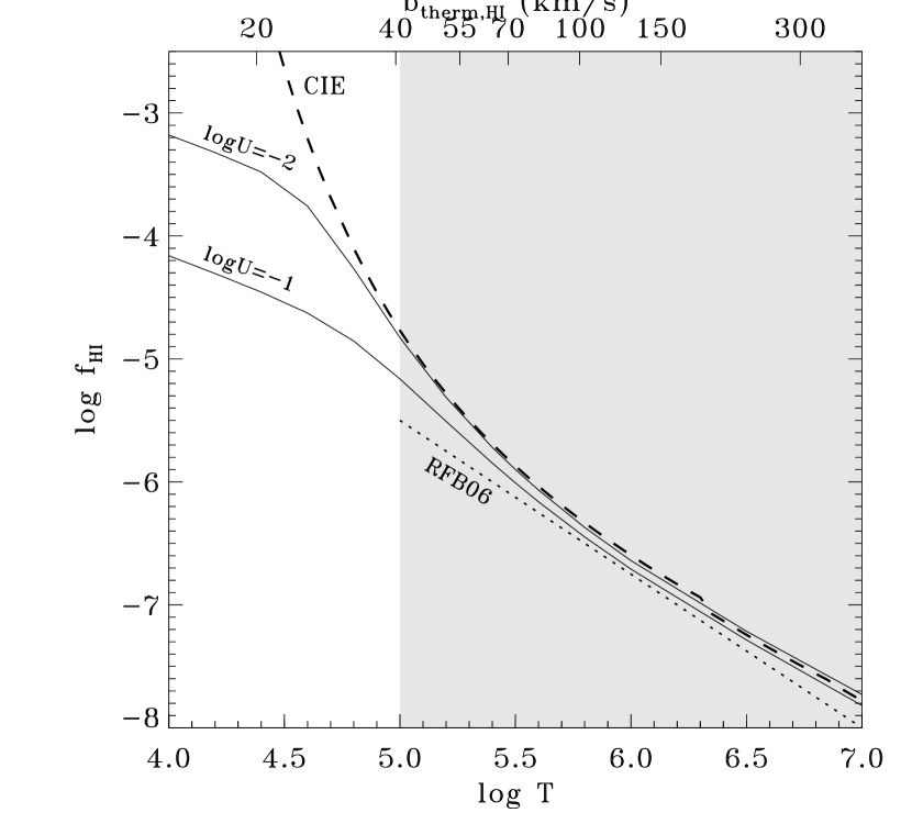
Using thermally-broadened H I lines to trace WHIM gas avoids many of the biases that can plague metal-ion based WHIM tracers (see Danforth, 2009). However, BLA surveys are fraught with observational complications as well (e.g. Richter et al., 2004, 2006). First, BLA lines are hard to detect and require spectra with a high signal-to-noise ratio (S/N) and minimal instrumental systematics. For example, at $T=10^{5}$ K, the hydrogen neutral fraction is approximately $f_{\rm HI}\sim 10^{-5}$ (Fig. 1) and the thermal $b$-value is 40 km s^-1 (Eq. 1). An IGM absorber with a total hydrogen (H I$+$H II) column density $N_{\rm H}=10^{18}$ cm^-2, typical of what is expected in the Ly$\alpha$ forest, would still have an observable H I column of $N_{\rm HI}\sim 10^{13}$ cm^-2. In the optically thin regime (linear COG of growth), the equivalent width $W_{\lambda}$ and line-center optical depth $\tau_{0}(N,T)$ for a Gaussian profile BLA are

$$W_{\lambda}(N)=\Bigl{(}\frac{\pi e^{2}}{m_{e}c}\Bigr{)}\,\Bigl{(}\frac{Nf\lambda^{2}}{c}\Bigr{)}=(54.5~{}{\rm m\AA})\,N_{13}$$ (2)

$$\tau_{0}(N,T)=\frac{\pi e^{2}}{m_{e}c}\frac{Nf\lambda^{2}}{\sqrt{\pi}b}=(0.187)\,N_{13}\,T_{5}^{-1/2},$$ (3)

where $N_{13}$ is the H I column density in units of $10^{13}$ cm^-2. Thus, an IGM absorber with $N_{13}\approx 1$ will have a rest-frame Ly$\alpha$ equivalent width $W_{\lambda}=55$ mÅ and a fractional depth of $\sim 20$% (assuming no non-thermal broadening). This line would be easily observable in data of modest S/N.

However the prospects get much worse at higher temperatures, as the thermal line width rises as $\sqrt{T}$ and the neutral fraction drops (Fig. 1). A Ly$\alpha$ absorber with the same total hydrogen column as above but with a temperature of $3\times 10^{5}$ K (near the peak CIE abundance of O VI) would have $f_{\rm HI}\sim 10^{-6}$, $N_{\rm HI}\sim 10^{12}$ cm^-2, $b=70$ km s^-1, $W_{\lambda}\sim 5$ mÅ, and a fractional depth $\tau_{0}\sim 1$%, impossible to detect unless the spectra have $S/N\gg 100$. Turbulent and/or bulk cloud motions would broaden the Ly$\alpha$ line even further and reduce the fractional line depth. Confirmation of a Ly$\alpha$ absorber and definitive measurements of $b_{\rm HI}$ and $N_{\rm HI}$ using higher Lyman lines and COG techniques are difficult for such lines since even Ly$\beta$ is a factor $\sim 7$ weaker than Ly$\alpha$ for unsaturated systems.

Figure 2.— Comparison of line width $b_{\rm LW}$ and COG doppler parameter $b_{\rm COG}$ in 164 Ly$\alpha$ absorbers from DS08. Top left: histogram of measured $b_{\rm LW}$ (dotted line) and $b_{\rm COG}$ (solid line). Bottom left: ratio $b_{\rm LW}/b_{\rm COG}$ covers a wide range, with a mean 1.35 and median $1.26^{+0.49}_{-0.25}$ (dotted lines). The top right panel shows that $b_{\rm LW}/b_{\rm COG}$ is weakly correlated with $b_{\rm LW}$ ($R=0.45$). Lower right panel shows that $b_{\rm LW}/b_{\rm COG}$ is uncorrelated with $\log\,N_{\rm HI}$ ($R=0.1$).

Detecting low-contrast absorption features depends critically on obtaining a correct model of the continuum level, as well as a presumption that the intrinsic continuum emanating from the AGN central engine is flat and featureless over these broad line widths. Since the UV continuum of Seyferts and QSOs is thought to arise in thermal accretion disk emission close to the central black hole, this requires that the accretion disk itself be featureless, which may or may not be a correct assumption. For this reason, the UV continua of BL Lac objects may provide better background sources for sensitive BLA detection. Additionally, fixed pattern noise and echelle-blazed gratings can themselves produce gentle undulations in the continuum, either on the detector or in the extraction process of curved orders imaged on rectilinear detectors and their corresponding artifacts and blemishes. The possible inability to place an accurate continuum due to the above difficulties not only makes low-contrast line detection suspect, but also makes it hard to set sensible detection limits as a function of $b$-value.

Even assuming data with sufficiently high S/N and a well-defined continuum, the identification of BLAs relies crucially on deconvolving the thermal line width $b_{\rm T}$ from the total observed line width $b_{\rm obs}$. A simple, single-component absorber can be modeled as a Voigt profile, and the observed line width is the quadrature sum of the thermal line width $b_{\rm T}$, the instrumental point spread function (usually approximated as a Gaussian $b_{\rm inst}$), and non-thermal broadening term $b_{\rm NT}$. The latter term encompasses bulk turbulence, multiple unresolved velocity components, or any other condition that will broaden a line profile. Instrumental broadening is generally well determined and can be subtracted from the total line width. However, the relative proportion of the thermal and non-thermal contributions is typically degenerate for absorption in a single species.

Some simulations (e.g., Richter, Fang, & Bryan, 2006) suggest that turbulence contributes on average $\sim 10$% to the total line width in broad absorbers, while other simulations suggest that it may be as much as 50% (Cen & Fang, 2006). Observational studies have shown that the line width measured from a single Ly$\alpha$ line is generally greater than that determined through a multi-Lyman-series COG (Shull et al., 2000). For example, the so-called Virgo Cluster absorbers in the high S/N GHRS spectrum of 3C 273 show a pair of Ly$\alpha$ components with measured $b=41$ km s^-1 and $34$ km s^-1 for the 1015 km s^-1 and 1590 km s^-1 IGM absorbers, respectively (Weymann et al., 1995). However, subsequent FUSE observations (Sembach et al., 2001) determined $b_{\rm COG}=30$ km s^-1 and 16 km s^-1 using three and eight higher-order Lyman lines, respectively.

While these absorbers make good individual examples, statistical studies show that $b$-values determined from line-width measurements of single lines, hereafter denoted $b_{\rm LW}$, systematically overpredict the true line width. Shull et al. (2000) found that $b_{\rm LW}/b_{\rm COG}\sim 2$ using Ly$\alpha$ and Ly$\beta$ measurements of 12 absorbers. Danforth et al. (2006) confirmed the low-$z$ result with a larger sample ($\sim 100$ absorbers). Similar conclusions were reached by Songaila (1997, 1998, 2001) for high-$z$ Ly$\alpha$ forest lines. We refine this relationship further using the large catalog of DS08. Out of $\sim 650$ H I absorbers in DS08 plus additions, we measured 164 in multiple Lyman lines, and a COG analysis was performed giving more accurate values of $b_{\rm HI}$ and $N_{\rm HI}$. Figure 2 shows the distribution of $b_{\rm Ly\alpha}$ and $b_{\rm COG}$ for this sample. Note that there is no clear correlation of $b_{\rm LW}/b_{\rm COG}$ with column density and only a weak trend with $b_{\rm LW}$. The median overprediction ratio is $b_{\rm LW}/b_{\rm COG}=1.26^{+0.49}_{-0.25}$ with a mean of 1.35. We will use this result extensively in our analysis for the BLAs in which only Ly$\alpha$ measurements are available.

Another impediment to BLA identification and measurement is that Ly$\alpha$ absorption lines often show ambiguous component structure. Several narrow components in a close blend can artificially broaden a line. Sometimes this will manifest itself as an asymmetric or obviously non-Gaussian line profile, but this blending can be undetectable even at arbitrarily high S/N and good spectral resolution. For this reason, even COG-determined $b$-values can overpredict the thermal line width.

Figure 3.— Blended absorption components in simulated STIS/E140M data. Two narrow components (left, $b_{1}=b_{2}=15$ km s^-1) separated by $\Delta v=b_{1}$ (component centroids marked with arrows) produce a combined profile which is indistinguishable from a single, broader component even in data of high S/N and resolution ($S/N=30$ per 7 km s^-1 resolution element). Fitting the profile as a single line gives $b_{\rm Ly\alpha}=19$ km s^-1 or a 27% overestimate of $b_{1}$. Even a COG analysis using Ly$\alpha$ and Ly$\beta$ profiles gives $b_{\rm COG}\sim 1.2\,b_{1}$. Doubling the line width of one component (right, $b_{2}=2\,b_{1}=30$ km s^-1) simulates a multiphase, broad + narrow system. The asymmetric profile makes it obvious that a single-component fit is not appropriate, but the component deconvolution and number of components are ambiguous.

To estimate the degree of line-width overprediction from COG analysis, we have modeled two simple two-component systems where the line width and relative centroid separation are varied (see also Danforth et al., 2006). In case 1 (Figure 3a), two narrow components, each with thermal line width $b_{\rm T}=15$ km s^-1, are blended into a single absorption line in Ly$\alpha$ and higher Lyman lines. The equivalent widths of each blended Lyman line are fitted with a COG. For component separation $\Delta v<b_{\rm T}$, the inferred $b_{\rm COG}$ overpredicts $b_{\rm T}$ by $<20\%$, but at $\Delta v>b_{\rm T}$, the overprediction rises to nearly 50%. This is largely independent of the relative column densities of the two lines. Depending on the strength of the line, the resolution of the spectrograph, and the quality of the data, even separations of $\Delta v>b_{\rm T}$ are not obvious in the line profile. Thus, a pair of narrow lines can easily be mistaken for a single broader system, even using a COG.

In case 2 (Figure 3b), we combine a narrow system ($b_{\rm T,1}=15$ km s^-1) with a broad absorber ($b_{\rm T,2}=2\,b_{\rm T,1}$) and vary the relative line strengths and component separations. For components of similar column density, $b_{\rm COG}$ is close to the mean of the two components, and separating the components by $(1-2)\,b_{\rm T,1}$ increases the composite $b_{\rm COG}$ by $\sim 20-50\%$ as in case 1. When one component is considerably stronger than the other, it dominates the $b_{\rm COG}$ solution. It is reassuring that the total column density of the composite system is conserved, independent of component separation and relative strength (Jenkins, 1986).

Appropriate to case 2, many observed absorbers classified as WHIM due to their O VI absorption are multiphase in nature (e.g., Danforth et al., 2006; Danforth & Shull, 2008; Tripp et al., 2008). A cool, photoionized component ($T<10^{5}$ K) is present at nearly the same velocity as a warm-hot component. We now estimate the broad Ly$\alpha$ profile expected to correspond with observed WHIM gas. For a typical O VI absorber with $N_{\rm OVI}\approx(10^{13.5}~{}{\rm cm^{-2}})\,N^{\rm(OVI)}_{13.5}$ at the peak CIE O VI abundance temperature ($T\approx T_{\rm max}=10^{5.45}$ K) the resulting BLA should have total hydrogen column density

$$N_{\rm hot}^{\rm(H)} = \frac{N_{\rm OVI}}{\langle f_{\rm OVI}\rangle(4.90\times 10^{-5})\,\bigl{(}\frac{Z}{0.1\,Z_{\sun}}\bigr{)}}$$ (4)

$$= (2.93\times 10^{18}~{}{\rm cm^{-2}})\,N_{13.5}^{\rm(OVI)}\,\Bigl{(}\frac{Z}{0.1\,Z_{\sun}}\Bigr{)}^{-1},$$

and, from Eq. 1, $b_{\rm HI}=(68.2~{}{\rm km~{}s^{-1}})\,(T/T_{\rm max})^{1/2}$. Here we adopt an oxygen abundance $(O/H)=(4.90\times 10^{-5})(Z/0.1Z_{\sun})$ scaled to 10% of the solar metallicity (Asplund et al., 2005). Given a typical neutral fraction $f_{\rm HI}\approx 1.4\times 10^{-6}$ at $T\approx T_{\rm max}$, the resulting BLA will have $N_{\rm HI}\sim 5\times 10^{12}$ cm^-2 and $\tau_{0}\sim 0.05$, easily overwhelmed by the narrower, stronger H I absorption from the photoionized component (typically $N_{\rm HI}\approx 10^{13-15}$ cm^-2, $b=20-30$ km s^-1, $\tau_{0}\gg 1$). The BLA signature will be apparent only in the line wings and will require exquisite data (S/N $\geq 30-40$) and a very good knowledge of the instrumental point spread function to recover.

Multiphase systems are difficult to identify individually, but there is statistical evidence for broad-plus-narrow H I systems (e.g., Tripp et al., 2001; Danforth & Shull, 2008; Tripp et al., 2008). DS08 compared the $b_{\rm HI}$ distribution of 83 H I systems with O VI detections with another 273 having clean O VI nondetections ($N_{\rm OVI}<10^{13.2}$ cm^-2). For the O VI detections, the median and standard deviation were $b_{\rm HI}=31\pm 15$ km s^-1, while the O VI nondetections show $b_{\rm HI}=26\pm 13$ km s^-1. This slight difference (at a low confidence level) suggests that weak BLA lines might be present in the O VI systems and broadening their overall H I profiles. However, it is doubtful whether a difference between the two populations would be apparent without the O VI detection “sign-posts”. There are several good, individual examples of this observational signature (e.g., Tripp, Savage, & Jenkins, 2000; Tripp et al., 2001; Stocke, Keeney, & Penton, 2005; Stocke et al., 2006).

Observing multiple Lyman lines and determining $b_{\rm HI}$ rigorously through a COG tends to produce more accurate line width measurements, but even here, multiple components can broaden a line width. Because the overestimate of the true $b_{\rm T}$ is smaller using a COG than for Ly$\alpha$ alone, we will adopt $b_{\rm COG}$ as our best estimator for absorber temperature. Examining higher-order Lyman lines cannot be counted on to solve the multi-component problem since most BLA absorbers are too weak to allow Ly$\beta$ to be detected and measured in all components. Nor will metal ions, which show intrinsically narrower lines, always help, since many BLAs are expected in regions of little or no metal enrichment. Thus, we must adopt a statistical approach to BLA verification.

Table 1BLA Sample Sight Lines

AGN	R.A.	Decl.	$z_{\rm AGN}$	$\Delta z_{\rm max}$	$\Delta X_{\rm max}$	Source
HE 0226$-$4110	02:28:15.2	$-$40:57:16	0.495	0.389	0.305	Lehner et al. (2006)
HS 0624$+$6907	06:30:02.5	$+$69:05:04	0.370	0.354	0.282	Aracil et al. (2006a, b)
PG 1116$+$215	11:19:08.6	$+$21:19:18	0.177	0.167	0.150	Sembach et al. (2004)
PG 1259$+$593	13:01:12.9	$+$59:02:07	0.478	0.388	0.303	Richter et al. (2004)
PKS 0405$-$123	04:07:48.4	$-$12:11:37	0.573	0.387	0.302	Lehner et al. (2007); Williger et al. (2006)
H 1821$+$643	18:21:57.3	$+$64:20:36	0.297	0.283	0.236	Sembach et al., in prep.
PG 0953$+$414	09:56:52.4	$+$41:15:22	0.234	0.225	0.195	Tripp et al., in prep.

2.2. Dataset and Methodology

With the above points in mind, we set out to determine what fraction of the reported BLAs are legitimately tracing warm-hot gas at $T\geq 10^{5}$ K. To accomplish this, we have independently extracted, reduced, and scrutinized the STIS/E140M spectra (Table 1) used by Lehner et al. (2007, L07 hereafter) to search for BLAs potentially arising in the WHIM. Complete details of our data reduction method are given in DS08. Briefly, STIS/E140M data were uniformly reduced using CalSTIS v2.19. Line-free continuum regions were defined interactively in 10Å segments of the data and fitted with low-order Legendre polynomials. Continuum fit uncertainty was taken as the standard deviation of points about the mean in the defined continuum region. This uncertainty was added in quadrature with those from photon noise and line fit uncertainties.

The L07 work is the most complete and comprehensive look at BLAs currently available. In order to determine the number and $b$-value distribution of BLA absorbers in the local universe, we have adopted the same definition as L07 and most other studies, requiring $T>10^{5}$ K corresponding to a hydrogen thermal $b>40$ km s^-1. The relationship between COG-determined line width and line width measured from a single line shows a median ratio $b_{\rm LW}/b_{\rm COG}=1.26^{+0.49}_{-0.25}$ in the large DS08 sample, and the correlation of that ratio with either $N_{\rm HI}$ or $b_{\rm LW}$ is poor (Fig. 2). Given this ratio, an absorber with $b_{\rm LW}\gtrsim 50$ km s^-1 (i.e., $1.26\times 40$ km s^-1) would be more likely than not to have a $b_{\rm COG}\geq 40$ km s^-1 (see Figure 2). Assuming that $b_{\rm COG}=b_{\rm T}$ (but, see discussion in Section 2.1). We find that $T\geq 10^{5}$ K for absorbers with line width $b_{\rm LW}\gtrsim 50$ km s^-1, not the $b_{\rm LW}\geq 40$ km s^-1 used by most previous works. This difference is central to our analysis. So as a guideline, we established the following categories and criteria for BLAs, using our analysis combined with that in the literature:

A. Probable BLA: There is no definitive test for BLAs, but we classify as “probable” any system with well-defined $b_{\rm COG}\geq 40$ km s^-1 or $b_{\rm LW}>60$ km s^-1 confirmed by independent measurement of L07 and ourselves and with no obvious sign of multiple component structure (such as an asymmetric profile) in Ly$\alpha$ or higher Lyman lines or metal ions (if available). Fifteen systems fall within this category. Note that we do not a priori use the presence or absence of O VI, N V, or other WHIM sign posts as a BLA determinant, although several O VI detections are present in this sample (see below).

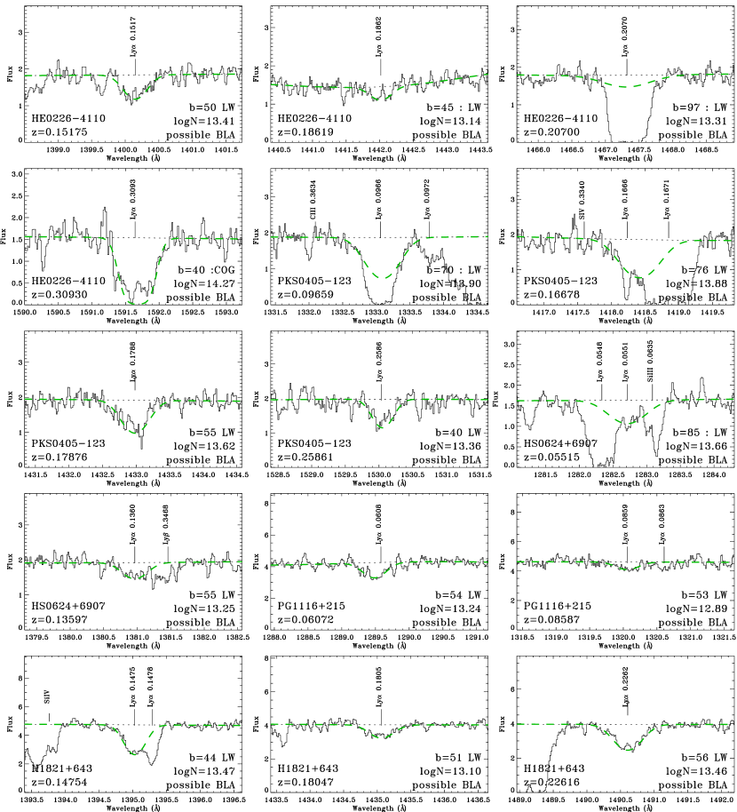
B. Possible BLA: Less likely than category A, the “possible” category includes systems with $40\leq b_{\rm LW}\leq 60$ km s^-1. This category also holds intermediate cases, where an absorber shows ambiguous component structure or a high degree of uncertainty as to line width and/or continuum fit, but a broad H I system component cannot be reasonably ruled out. Forty-eight H I absorbers fall in this category.

Figure 4.— Examples of three purported Ly$\alpha$ lines that do not appear in our reduction of the STIS/E140M data. Reported redshifts, $b$-values, and column densities listed in L07 are printed in the lower left corner of each panel, and the resulting line profiles are overplotted. Most of these “missing” lines are associated with very narrow bad-pixel regions where the flux drops to negative values in our version of the reduced data.

Figure 5.— Potential “echelle ripple” behavior at the long-wavelength end of the STIS/E140M detector. Four Ly$\alpha$ absorbers are claimed (Lehner et al., 2006) but only the reddest ($z=0.40027$) is confirmed with a Ly$\beta$ counterpart. While we view the other three absorbers with some skepticism, we find little or no similar “echelle ripple” behavior in other datasets and retain them as possible BLAs in our accounting.

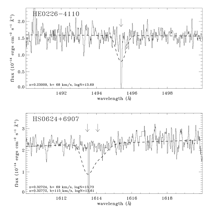
C. Non-BLA: Nearly half (56/119) of the H I lines with $b\geq 40$ km s^-1 published by L07 or DS08 are most likely not BLAs by our assessment for a variety of reasons: measured $b_{\rm COG}<40$ km s^-1 or $b_{\rm LW}<40$ km s^-1; probable alternate line identification; obvious narrow component structure; or simply not detected as absorption features in our reduction of the data (i.e., we do not confirm the extraction and/or analysis done by or referenced in L07, see Figure 4). The last group, encompassing nine purported absorbers, occurs primarily in the spectrum of HS 0624$+$6907 (Aracil et al., 2006a, b). In the course of our independent analysis, we identified a few BLA candidates that were not listed in L07 or other independent literature sources. In most cases, these lines turn out to be something other than Ly$\alpha$ and thus fall into category C, as they are not confirmed by two independent sources.

Because the 7 individual sightlines were analyzed originally by different authors, somewhat differing analysis procedures were used and then adopted by L07. Each is briefly discussed below, with notes that bear on the BLA identification process.

HE 0226$-$4110

Originally analyzed by Lehner et al. (2006), the spectrum is shown in that paper. No COG measurements are reported; instead some $b$-values are obtained by simultaneous fitting of several Lyman-series lines (see discussion below). Longward of 1690 Å, the continuum in this spectrum appears to “ripple” in both our extracted spectrum (Figure 5) that of Lehner et al.. This gives rise to four reported BLA candidates (one with $b_{\rm LW}\sim 150$ km s^-1) in only $\Delta z=0.007$. The periodic nature of these features are suspicious, especially given that these features occur the highest spectral orders which cut across many detecor rows before extraction. However, no similar features appear in the highest spectral order ($1690<\lambda<1710$Å) for AGN where $z_{\rm Ly\alpha}>z_{\rm AGN}$.

HS 0624$+$6907

Originally analyzed by Aracil et al. (2006a, b), no spectra were published. These authors do not mention obtaining COG $b$-values except for a Ly$\alpha$ absorption complex at $z\sim 0.06$. Therefore, we assume that all $b$-values quoted by L07 for this spectrum are either Ly$\alpha$ line width values or simultaneous line width fits to two or more Lyman lines as described for HE 0226$-$4110 above. Several of the BLAs reported by L07 in this sight line are at or near the locations of detector artifacts; we see no believable absorption at these locations based on our own reduction of the data. The reported lines may be a result of smoothing the data over these bad pixels. Longward of 1580 Å in this spectrum our extracted data does not match even the presence of some of the absorption lines listed by L07 (Figure 4). These unconfirmed lines are listed in Table 2 as non-BLAs for completeness, but are not otherwise analyzed.

PG 1116$+$215

Originally analyzed by Sembach et al. (2004), the spectrum is shown in that paper. Sembach et al. (2004) use COG $b$-values where available, although none apply to the BLAs in this sight line.

PG 1259$+$593

This sight line was originally analyzed by Richter et al. (2004) and the spectrum is shown in that paper. Richter et al. list several COG $b$-values for BLAs and we add several more.

PKS 0405$-$123

Originally analyzed by Williger et al. (2006, W06) and reanalyzed by L07. Neither W06 nor L07 report COG measurements for this sightline. The spectrum is shown in Williger et al.  Despite mentioning that the reanalysis was required due to the large number of suspect BLA candidates, L07 $b$-values from simultaneous line fits are similar to the Ly$\alpha$-only line-widths reported by Williger et al. (2006). We report several COG $b$-values for this sight line and, similar to many other absorption systems we generally find $b_{\rm COG}\leq b_{\rm LW}$ (see below).

H 1821$+$643

For spectral analysis, L07 refer to Sembach et al. In prep. which does not appear to have been published yet. There is no mention of COG measurements in the L07 description, so we have assumed that the reported values are $b_{\rm LW}$.

PG 0953$+$415

L07 report these BLAs based upon an unpublished Tripp et al. analysis. We have assumed that all quoted $b$-values are based on Ly$\alpha$ line width measurements since our own $b_{\rm LW}$ values are similar.

One of the procedural differences between L07 and the current work is that where more than one Lyman line is detected in absorption in these spectra, we have used a $b$-value determined by the COG method whereas L07 uses a simultaneous line fit of all available lines. In general, the $b_{\rm COG}$ values are significantly smaller than those obtained by the simultaneous line fitting method. To evaluate this difference, we have used the 10 absorbers in the PKS 0405$-$123 sight line analyzed independently by ourselves, L07, and W06. For all ten systems the W06 ($b_{\rm LW}$) measurements agree to within the errors with the L07 (simultaneous line-fits) $b$-values. Half of these measurements also show excellent agreement with $b_{\rm COG}$. However, the other five systems show $b_{\rm COG}$ values significantly less than values obtained by the simultaneous line fit method (for details see Table 2) and these disagreements are for the largest $b$-values reported by L07 in this sightline. Three systems ($z=0.09659$, $0.16121$, and $0.32500$) have COG $b$-values with tight error bars half or less of the L07 reported values; two other systems ($z=0.17876$ and $0.25861$) have similar differences between reported values but, with large $b_{\rm COG}$ error bars and so are not inconsistent with the large line widths reported by L07. Based upon these 10 systems only, we find significant differences between COG $b$-values and simultaneous line-fit $b$-values in roughly half the cases, all in the sense that the COG $b$-values are significantly less (35-50% the amount). When higher S/N FUV spectra from COS become available, tests using these two techniques should be made to determine which method is the most reliable as a function of line width and S/N.

3. Results

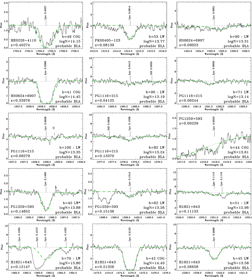
All BLA candidates drawn from the catalogs of L07 and DS08 were independently analyzed by both Danforth and Stocke based on the criteria above. In Table 2, we list the Probable (A), Possible (B), and non-BLA (C) absorbers based upon our analyses. Sight line name and absorber redshift are in the first two columns. Independent $b$-values and column densities are listed from L07 (or similar source, columns 3-5) and DS08/this work (columns 6-8). COG measurements of $b_{\rm HI}$, $N_{\rm HI}$ are given where possible, otherwise the unweighted mean of the two independent Ly$\alpha$ measurements is taken as consensus $b$, $N_{\rm HI}$ values along with the method used (‘LW’ for Ly$\alpha$ line width; ‘COG’ for curve of growth) in columns 9 and 10. Brief notes are given for each absorber, with additional details presented in an Appendix for many absorbers in column 11. In total, we find 15 absorbers in group A (Probable BLAs) and 48 in group B (Possible BLAs) and 56 non-BLAs out of 119 candidate systems with $b>40$ km s^-1 as reported by L07, DS08, or similar literature source. We show the Probable BLAs in Figure 6 and a selection of Possible BLAs in Figure 7.

Table 2Probable, Possible, and non-BLA Absorbers

Sight Line	$z_{\rm abs}$	$b_{1}$	log $N_{1}$	Src	$b_{2}$	log $N_{2}$	Src	$b_{0}$	log $N_{0}$	Absorber Notes
		(km s-1)	(cm-2)	1	(km s-1)	(cm-2)	2	(km s-1)	(cm-2)
Probable BLA Detections
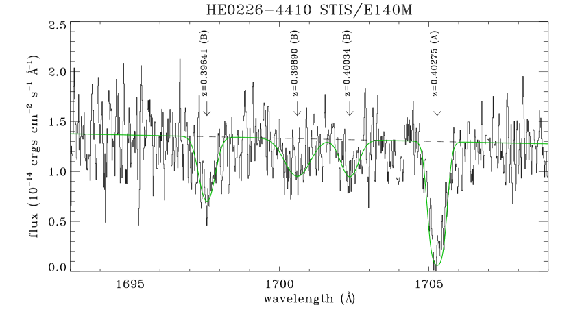
HE 0226$-$4110	0.40274	$46\pm 4$	$14.13\pm 0.04$	L07	$49$ COG	$14.16\pm 0.11$	DS08	49 COG	14.15	Ly$\alpha$,$\beta$ detections
PKS 0405$-$123	0.08139	$54\pm 4$	$13.79\pm 0.02$	L07	$53\pm 2$	$13.76\pm 0.02$	DS08	53 LW	13.77	see appendix
HS 0624$+$6907	0.09023	$76\pm 14$	$13.29\pm 0.08$	L07	$100:$	$13.34\pm 0.04$	this	90: LW	13.31	very weak and broad
HS 0624$+$6907	0.33976	$42\pm 1$	$14.45\pm 0.03$	L07	$41$ COG	$14.46^{+0.10}_{-0.03}$	DS08	41 COG	14.45	OVI, see appendix
PG 1116$+$215	0.04125	$105\pm 18$	$13.25^{+0.11}_{-0.09}$	L07	$72\pm 6$	$13.13^{+0.06}_{-0.05}$	DS08	90: LW	13.19	very weak
PG 1116$+$215	0.06244	$77\pm 9$	$13.18^{+0.07}_{-0.06}$	L07	$65\pm 7$	$13.10\pm 0.06$	this	71 LW	13.14	very weak
PG 1116$+$215	0.09279	$133\pm 17$	$13.39^{+0.09}_{-0.08}$	L07	$83:$	$13.31^{+0.04}_{-0.03}$	this	100: LW	13.35	see appendix
PG 1116$+$215	0.13370	$84\pm 10$	$13.27^{+0.08}_{-0.07}$	L07	$79\pm 6$	$13.20\pm 0.04$	DS08	82 LW	13.24	OVI, see appendix
PG 1259$+$593	0.00229	$44^{+9}_{-4}$ COG	$13.61\pm 0.06$	R04	$61\pm 5$	$13.83\pm 0.24$	this	44 COG	13.61	see appendix
PG 1259$+$593	0.14852	$42\pm 2$	$13.91\pm 0.06$	L07	$57:$ COG	$13.85\pm 0.01$	this	42 LW*	13.88	see appendix
PG 1259$+$593	0.15136	$65\pm 6$	$13.32\pm 0.09$	L07	$59\pm 5$	$13.21\pm 0.05$	DS08	62 LW	13.26
H 1821$+$643	0.11133	$88\pm 14$	$12.95^{+0.10}_{-0.13}$	L07	$51:$	$12.97\pm 0.03$	this	51: LW	12.96	see appendix
H 1821$+$643	0.12147	$40^{+44}_{-21}$	$14.04\pm 0.36$	L07	$76\pm 5$	$13.79\pm 0.06$	this	70: LW	13.80	OVI, see appendix
H 1821$+$643	0.21326	$43\pm 2$	$14.41^{+0.04}_{-0.04}$	L07	$42^{+5}_{-4}$ COG	$14.40^{+0.08}_{-0.09}$	DS08	42 COG	14.40	OVI, see appendix
H 1821$+$643	0.26658	$45\pm 2$	$13.64^{+0.03}_{-0.03}$	L07	$45\pm 1$	$13.52\pm 0.01$	DS08	45 LW	13.58	OVI, see appendix
Possible BLA Detections
HE 0226$-$4110	0.06083	$45\pm 1$	$14.65\pm 0.02$	L07	$46\pm 15$	$14.86\pm 0.15$	this	45 LW	14.75	see appendix
HE 0226$-$4110	0.09220	$40\pm 18$	$12.94\pm 0.11$	L07	$47\pm 9$	$13.11^{+0.08}_{-0.05}$	this	44 LW	13.03	weak, profile uncertain
HE 0226$-$4110	0.15175	$49\pm 7$	$13.42\pm 0.05$	L07	$51\pm 5$	$13.39\pm 0.03$	this	50 LW	13.41	asymmetric
HE 0226$-$4110	0.16339	$46\pm 2$	$14.36\pm 0.04$	L07	$39\pm 7$	$14.34\pm 0.03$	this	42 LW	14.35	see appendix
HE 0226$-$4110	0.18619	$54\pm 16$	$13.26\pm 0.08$	L07	$37\pm 8$	$13.02\pm 0.07$	this	45: LW	13.14	possibly two components
HE 0226$-$4110	0.20700	$97:$	$13.31\pm 0.39$	S05	blend	$<15.20$	this	97: LW	13.31	OVI, NeVIII, see appendix
HE 0226$-$4110	0.30930	$44\pm 2$	$14.26\pm 0.03$	L07	$38^{+21}_{-9}$ COG	$14.28^{+0.20}_{-0.17}$	this	40:COG	14.27	see appendix
HE 0226$-$4110	0.39641	$63\pm 23$	$13.59\pm 0.10$	L07	$57\pm 10$	$13.54\pm 0.10$	this	60 LW	13.57	see appendix
HE 0226$-$4110	0.39890	$152:$	$13.50\pm 0.16$	L07	$88\pm 20$	$13.46\pm 0.10$	this	100: LW	13.50	see appendix
HE 0226$-$4110	0.40034	$61\pm 26$	$13.39\pm 0.11$	L07	$74\pm 16$	$13.29\pm 0.11$	this	70 LW	13.34	see appendix
PKS 0405$-$123	0.03196	$54\pm 16$	$13.33\pm 0.08$	L07	$57\pm 8$	$13.33\pm 0.06$	DS08	56 LW	13.33	see appendix
PKS 0405$-$123	0.07523	$48\pm 20$	$13.05\pm 0.11$	L07	$37\pm 12$	$12.81\pm 0.13$	this	43 LW	12.93	see appendix
PKS 0405$-$123	0.09659	$70\pm 20$	$13.90\pm 0.18$	L07	$36\pm 4$ COG	$14.64^{+0.12}_{-0.11}$	DS08	70: LW	13.90	OVI, see appendix
PKS 0405$-$123	0.13102	$52\pm 8$	$13.46\pm 0.05$	L07	$53\pm 6$	$13.35\pm 0.04$	this	57 LW	13.41	see Appendix
PKS 0405$-$123	0.13377	$43\pm 8$	$13.34\pm 0.06$	L07	$45\pm 7$	$13.22\pm 0.07$	this	44 LW	13.28	see Appendix
PKS 0405$-$123	0.16678	$75\pm 7$	$13.91\pm 0.04$	L07	$77\pm 7$	$13.84\pm 0.05$	this	76 LW	13.88	poss. OVI, see appendix
PKS 0405$-$123	0.17876	$55\pm 7$	$13.61\pm 0.04$	L07	$18^{+44}_{-7}$ COG	$13.92^{+0.29}_{-0.31}$	DS08	55 LW	13.62	asymetric, see appendix
PKS 0405$-$123	0.18269	$48\pm 2$ COG	$15.07\pm 0.09$	W06	$49^{+10}_{-6}$ COG	$14.90^{+0.15}_{-0.20}$	DS08	49 COG	14.86	OVI, see appendix
PKS 0405$-$123	0.19086	$44\pm 16$	$13.17\pm 0.09$	L07	$38\pm 9$	$13.01^{+0.10}_{-0.06}$	this	41 LW	13.09	see Appendix
PKS 0405$-$123	0.24513	$54\pm 24$	$13.23\pm 0.11$	L07	$30\pm 5$	$13.01\pm 0.09$	this	42: LW	13.12	poor agreement, see appendix
PKS 0405$-$123	0.25861	$40\pm 9$	$13.37\pm 0.07$	L07	$39\pm 4$	$13.36^{+0.15}_{-0.10}$	this	40 LW	13.36	$b_{\rm COG}=21^{+25}_{-10}$; W06:$b_{\rm LW}=47\pm 7$
PKS 0405$-$123	0.29523	$47\pm 13$	$13.33\pm 0.08$	L07	$39\pm 8$	$13.07\pm 0.08$	this	43 LW	13.20
PKS 0405$-$123	0.29904	$49\pm 23$	$13.26\pm 0.12$	L07	$54\pm 10$	$13.14\pm 0.15$	this	52: LW	13.20	noisy, components?
PKS 0405$-$123	0.35092	$38\pm 2$	$14.25\pm 0.03$	L07	$56\pm 15$ COG	$14.04\pm 0.08$	DS08	40: LW	14.25	see appendix
PKS 0405$-$123	0.40886	$40\pm 2$	$14.38\pm 0.03$	L07	$40^{+7}_{-4}$ COG	$14.32\pm 0.05$	DS08	40:COG	14.35	see appendix
HS 0624$+$6907	0.05437	$60\pm 19$	$13.09\pm 0.11$	L07	$45\pm 5$	$12.88^{+0.13}_{-0.11}$	this	52: LW	12.99	see appendix
HS 0624$+$6907	0.05515	$84\pm 31$	$13.68\pm 0.17$	L07	$87\pm 13$	$13.69\pm 0.06$	this	85: LW	13.66	see appendix
HS 0624$+$6907	0.13597	$57\pm 11$	$13.33\pm 0.10$	L07	$52\pm 12$	$13.16\pm 0.10$	this	55 LW	13.25	OVI, see appendix
HS 0624$+$6907	0.21323	$45\pm 6$	$13.22\pm 0.05$	L07	$40\pm 7$	$13.04\pm 0.08$	DS08	43 LW	13.13	poss. SiIII, CIII
HS 0624$+$6907	0.26856	$51\pm 7$	$13.03\pm 0.05$	L07	$46\pm 8$	$13.00\pm 0.07$	this	49 LW	13.02	weak
HS 0624$+$6907	0.29661	$52\pm 3$	$13.54\pm 0.02$	L07	$45$	$13.31\pm 0.04$	DS08	48 LW	13.43
HS 0624$+$6907	0.30994	$66\pm 12$	$13.61\pm 0.10$	L07	$38\pm 9$	$12.90\pm 0.11$	DS08	52: LW	13.25	poss. OVI, see appendix
HS 0624$+$6907	0.31790	$34\pm 4$	$13.37\pm 0.04$	L07	$51\pm 7$	$13.38^{+0.07}_{-0.05}$	DS08	43 LW	13.38	OVI, see appendix
PG 0953$+$415	0.05879	$63^{+19}_{-14}$	$13.41\pm 0.16$	L07	not measured	not measured	$\cdots$	63: LW	13.37	see appendix
PG 0953$+$415	0.17985	$48^{+11}_{-9}$	$13.27\pm 0.07$	L07	$48\pm 2$	$13.20^{+0.07}_{-0.05}$	DS08	48 LW	13.24	see appendix
PG 0953$+$415	0.19126	$48^{+95}_{-32}$	$13.08\pm 0.55$	L07	$66:$	$13.50\pm 0.04$	this	40: LW	13.30	see appendix
PG 0953$+$415	0.20104	$71^{+41}_{-26}$	$13.16\pm 0.16$	L07	$44:$	$12.63\pm 0.19$	this	57: LW	12.90	weak, uncertain continuum
PG 1116$+$215	0.01638	$49\pm 5$	$13.39\pm 0.06$	L07	$54\pm 4$	$13.44\pm 0.03$	DS08	51 LW	13.41	asymmetric
PG 1116$+$215	0.06072	$55\pm 6$	$13.28^{+0.06}_{-0.05}$	L07	$53$	$13.21\pm 0.04$	DS08	54 LW	13.24
PG 1116$+$215	0.08587	$52\pm 14$	$12.90^{+0.19}_{-0.13}$	L07	$55\pm 11$	$12.88\pm 0.08$	this	53 LW	12.89	see appendix
PG 1259$+$593	0.19573	$43\pm 7$	$13.07\pm 0.14$	R04	$46\pm 19$	$13.05\pm 0.15$	DS08	44 LW	13.06	see appendix
PG 1259$+$593	0.41786	$51\pm 4$	$13.25\pm 0.08$	L07	$52\pm 24$	$13.23\pm 0.18$	DS08	51: LW	13.24	asymmetric
H 1821$+$643	0.02642	$49\pm 6$	$13.26^{+0.07}_{-0.08}$	L07	$44\pm 3$	$13.19\pm 0.03$	DS08	47 LW	13.23	asymmetric
H 1821$+$643	0.14754	$45\pm 3$	$13.51^{+0.03}_{-0.03}$	L07	$42\pm 2$	$13.43\pm 0.02$	this	44 LW	13.47	see appendix
H 1821$+$643	0.16352	$52\pm 6$	$13.17^{+0.06}_{-0.07}$	L07	$56\pm 4$	$13.11\pm 0.04$	DS08	54 LW	13.14	weak, slightly asymmetric
H 1821$+$643	0.18047	$51\pm 7$	$13.14^{+0.07}_{-0.08}$	L07	$52\pm 8$	$13.05\pm 0.07$	DS08	51 LW	13.10
H 1821$+$643	0.22616	$55\pm 4$	$13.51^{+0.04}_{-0.04}$	L07	$56\pm 2$	$13.41\pm 0.07$	this	56 LW	13.46	offset OVI, see appendix
H 1821$+$643	0.25814	$60\pm 9$	$13.38^{+0.10}_{-0.13}$	L07	$56:$	$13.26\pm 0.04$	this	58: LW	13.32	see appendix
Not BLAs
HE 0226$-$4110	0.01216	not detected	not detected	$\cdots$	$41\pm 7$	$13.06^{+0.08}_{-0.07}$	DS08	$\cdots$	$\cdots$	poor S/N, not confirmed
HE 0226$-$4110	0.02679	$42\pm 11$	$13.22\pm 0.08$	L07	$30\pm 4$	$13.17^{+0.12}_{-0.05}$	DS08	36 LW	13.19	Lehner et al. 2006:$b_{\rm LW}=28$
HE 0226$-$4110	0.23009	$68\pm 8$	$13.69\pm 0.04$	L07	not detected	not detected	$\cdots$	$\cdots$	$\cdots$	no absorption seen
HE 0226$-$4110	0.22102	$34\pm 18$	$12.99\pm 0.12$	L07	$44\pm 9$	$13.06^{+0.07}_{-0.08}$	this	39 LW	13.02	weak
HE 0226$-$4110	0.38420	$62\pm 7$	$13.91\pm 0.04$	L07	$31:$ COG	$13.08^{+0.11}_{-0.10}$	this	31: COG	13.49	components, see appendix
PKS 0405$-$123	0.05896	$77\pm 27$	$13.34\pm 0.10$	L07	$20,20$	$12.97\pm 0.08$	this	20 LW	12.97	see appendix
PKS 0405$-$123	0.07218	$45\pm 14$	$13.09\pm 0.08$	L07	$45:$	$13.01\pm 0.06$	this	45 LW	13.05	see appendix
PKS 0405$-$123	0.10298	$87\pm 19$	$13.40\pm 0.07$	L07	$54:$	$13.35^{+0.04}_{-0.03}$	this	70: LW	13.38	see appendix
PKS 0405$-$123	0.10419	not detected	not detected	$\cdots$	$48\pm 5$	$12.98\pm 0.08$	DS08	$\cdots$	$\cdots$	see appendix
PKS 0405$-$123	0.13646	$54\pm 11$	$13.34\pm 0.06$	L07	$11,19$	$12.96\pm 0.07$	this	19: LW	12.96	see appendix
PKS 0405$-$123	0.13924	$35\pm 11$	$13.02\pm 0.11$	W06	$53\pm 2$	$13.13^{+0.06}_{-0.05}$	DS08	44 LW	13.08	see appendix
PKS 0405$-$123	0.15304	$46\pm 3$	$13.80\pm 0.03$	L07	$50:$	$13.76\pm 0.03$	this	48: LW	13.78	see appendix
PKS 0405$-$123	0.16121	$54\pm 8$	$13.71\pm 0.04$	L07	$27\pm 14$ COG	$13.62^{+0.31}_{-0.15}$	DS08	27 COG	13.66	see appendix
PKS 0405$-$123	0.16714	$30\pm 1$	$16.27\pm 0.13$	L07	$40^{+12}_{-7}$ COG	$15.47^{+0.40}_{-0.48}$	DS08	$\cdots$	$\cdots$	OVI, components, see appendix
PKS 0405$-$123	0.24057	$57\pm 19$	$13.27\pm 0.09$	L07	$58\pm 6$	$13.27^{+0.08}_{-0.07}$	this	58 LW	13.27	marginal feature, artifact
PKS 0405$-$123	0.28838	$52\pm 19$	$13.32\pm 0.10$	L07	$30:$	$13.18\pm 0.10$	this	30: LW	13.10	components; W06:$b_{\rm LW}=27\pm 7$
PKS 0405$-$123	0.32500	$66\pm 13$	$13.55\pm 0.06$	L07	$60:$	$13.45^{+0.04}_{-0.08}$	this	63: LW	13.50	see appendix
PKS 0405$-$123	0.34234	$42\pm 13$	$13.39\pm 0.08$	L07	$35\pm 4$	$13.27^{+0.07}_{-0.05}$	this	38 LW	13.33	asymetric
PKS 0405$-$123	0.36150	$44\pm 10$	$13.71\pm 0.10$	L07	$25\pm 3$ COG	$15.18\pm 0.13$	this	30: COG	15.00	see appendix
HS 0624$+$6907	0.04116	$41\pm 3$	$13.33\pm 0.03$	L07	not measured	not measured	$\cdots$	$\cdots$	$\cdots$	SIII$z=0.0635$, see appendix
HS 0624$+$6907	0.05483	$35:$	$14.50:$	L07	$45^{+28}_{-9}$ COG	$14.28^{+0.11}_{-0.15}$	DS08	35: LW	14.28	see appendix
HS 0624$+$6907	0.06346	$48\pm 8$	$14.46\pm 0.30$	L07	$33^{+2}_{-1}$ COG	$15.25^{+0.10}_{-0.06}$	DS08	33 COG	15.25	OVI, see appendix
HS 0624$+$6907	0.19979	$17\pm 2$	$13.24\pm 0.05$	L07	$55\pm 10$	$13.58\pm 0.03$	DS08	17 LW	13.41	poss. OVI; components in Ly$\beta$
HS 0624$+$6907	0.21990	$60\pm 9$	$13.39\pm 0.05$	L07	not detected	not detected	$\cdots$	$\cdots$	$\cdots$	not detected
HS 0624$+$6907	0.23231	$44\pm 8$	$13.33\pm 0.08$	L07	not detected	not detected	$\cdots$	$\cdots$	$\cdots$	not detected
HS 0624$+$6907	0.28017	$43\pm 2$	$14.32\pm 0.02$	L07	$35^{+6}_{-5}$ COG	$14.42^{+0.09}_{-0.07}$	DS08	35 COG	14.37
HS 0624$+$6907	0.29531	$42\pm 2$	$13.80\pm 0.02$	L07	$34$	$13.62\pm 0.03$	DS08	38 LW	13.71
HS 0624$+$6907	0.31045	$62\pm 40$	$13.43\pm 0.33$	L07	not detected	not detected	$\cdots$	$\cdots$	$\cdots$	see appendix
HS 0624$+$6907	0.31088	$51\pm 28$	$13.13\pm 0.43$	L07	not detected	not detected	$\cdots$	$\cdots$	$\cdots$	see appendix
HS 0624$+$6907	0.31280	$54\pm 9$	$13.65\pm 0.10$	L07	not detected	not detected	$\cdots$	$\cdots$	$\cdots$	not detected
HS 0624$+$6907	0.31326	$55\pm 11$	$13.62\pm 0.10$	L07	not detected	not detected	$\cdots$	$\cdots$	$\cdots$	not detected
HS 0624$+$6907	0.32089	$31\pm 1$	$13.97\pm 0.02$	L07	$44^{+13}_{-14}$ COG	$13.80^{+0.06}_{-0.11}$	DS08	31 LW	13.89	see appendix
HS 0624$+$6907	0.32724	$69\pm 16$	$13.73\pm 0.32$	L07	not detected	not detected	$\cdots$	$\cdots$	$\cdots$	not detected
HS 0624$+$6907	0.32772	$115\pm 62$	$13.61\pm 0.43$	L07	not detected	not detected	$\cdots$	$\cdots$	$\cdots$	not detected
PG 0953$+$415	0.02336	$56^{+14}_{-11}$	$13.21\pm 0.08$	L07	$20:$	$12.68^{+0.19}_{-0.12}$	this	38: LW	12.95	discrepant measurements
PG 0953$+$415	0.04382	not detected	not detected	$\cdots$	$47\pm 8$	$13.39^{+0.03}_{-0.04}$	DS08	47 LW	13.06	OVI$z=0.22974$; see appendix
PG 0953$+$415	0.12784	$44:$	$12.83\pm 0.35$	L07	not detected	not detected	this	$\cdots$	$\cdots$	not detected, see appendix
PG 0953$+$415	0.19361	$40\pm 2$	$13.94\pm 0.02$	L07	$37\pm 2$	$13.82\pm 0.03$	this	39 COG	14.15	see appendix
PG 0953$+$415	0.20006	$66^{+18}_{-14}$	$13.24\pm 0.09$	L07	$32\pm 7$	$12.91\pm 0.11$	DS08	49: LW	13.07	continuum uncertainties
PG 1116$+$215	0.02841	$31\pm 1$	$13.80\pm 0.02$	L07	$43:$	$13.71^{+0.21}_{-0.09}$	DS08	35 LW	13.78
PG 1116$+$215	0.05904	$21,30$	???	S04	$45:$	$13.53\pm 0.02$	DS08	21,30 LW	13.53	components
PG 1259$+$593	0.04606	$48\pm 12$	$15.58\pm 0.21$	L07	$30^{+10}_{-8}$ COG	$15.51^{+0.28}_{-0.25}$	DS08	32 COG	15.55	OVI, components, see appendix
PG 1259$+$593	0.06931	not detected	not detected	$\cdots$	$54\pm 4$	$13.33\pm 0.04$	DS08	54 LW	13.33	not detected by R04
PG 1259$+$593	0.08041	$42\pm 4$	$12.97\pm 0.10$	L07	$26\pm 2$	$12.86$	this	34: LW	12.92	not detected by R04
PG 1259$+$593	0.17891	$99\pm 9$	$13.29\pm 0.10$	L07	not measured	not measured	$\cdots$	$\cdots$	$\cdots$	not detected
PG 1259$+$593	0.21136	not measured	not measured	$\cdots$	$47\pm 3$	$13.39\pm 0.04$	DS08	47 LW	13.39	see appendix
PG 1259$+$593	0.22861	$40\pm 3$	$13.47\pm 0.05$	L07	$34\pm 2$	$13.42\pm 0.03$	DS08	37 LW	13.44
PG 1259$+$593	0.24126	$89\pm 7$	$13.41\pm 0.09$	L07	$23\pm 4$	$12.86\pm 0.08$	this	55 LW	13.14	ambiguous components
PG 1259$+$593	0.25971	$41\pm 5$	$13.84\pm 0.12$	L07	$29^{+7}_{-5}$ COG	$13.98\pm 0.07$	DS08	29 COG	13.91	OVI, obvious components
PG 1259$+$593	0.30434	$65\pm 1$	$13.76\pm 0.14$	L07	$20^{+8}_{-3}$ COG	$13.81^{+0.07}_{-0.09}$	DS08	20 COG	13.81	obvious components
PG 1259$+$593	0.31978	$74\pm 8$	$13.98\pm 0.06$	L07	$31\pm 3$ COG	$14.07^{+0.01}_{-0.06}$	DS08	31 COG	14.07	OVI; listed as blend in R04
PG 1259$+$593	0.32478	$46\pm 10$	$13.24\pm 0.15$	L07	$20$	$12.93^{+0.14}_{-0.11}$	DS08	33: LW	13.10	OVI; continuum uncertainty?
PG 1259$+$593	0.43569	$44\pm 4$	$14.22\pm 0.10$	R04	$\cdots$	$\cdots$	$\cdots$	$\cdots$	$\cdots$	see appendix
H 1821$+$643	0.12221	$42\pm 4$	$13.19\pm 0.06$	L07	$34\pm 5$	$13.13^{+0.03}_{-0.04}$	DS08	38 LW	13.16
H 1821$+$643	0.19176	not detected	not detected	$\cdots$	$47\pm 7$	$12.72\pm 0.07$	DS08	$\cdots$	$\cdots$	marginal; not confirmed by L07
H 1821$+$643	0.22480	not detected	not detected	$\cdots$	$40^{+6}_{-8}$ COG	$15.41^{+0.25}_{-0.08}$	DS08	40 COG	15.41	OVI; components, see appendix

Figure 6.— Spectra of all 15 Probable BLA systems illustrate the diversity of line profiles. The sight line and absorber redshift are listed on the left side of each panel while the consensus $b$ (km s^-1) and $\log\,N$ values from Table 2 are listed on the right. Dotted line shows continuum fit to the data, and dashed curve shows consensus absorption profile. Adjacent line detections are indicated with vertical ticks and labeled with ion and redshift. Lines identified without redshift denote Galactic interstellar absorption. Flux is in units of $10^{-14}\rm~{}erg~{}cm^{-2}~{}s^{-1}~{}\AA^{-1}$. See Table 2 and Appendix for more details of individual systems.

Figure 7.— Same as Fig. 6 but for 15 of the 48 Possible BLA systems. Additional Possible BLAs are shown in Figure 10.

3.1. Broad Ly$\alpha$ Absorber Frequency

In measuring metal-ion absorption lines, DS08 employ a $4\sigma$ detection limit, with equivalent width

$$W_{\rm obs}\geq\frac{(SL)~{}(\lambda/R)}{(S/N)_{\lambda}},$$ (5)

where the instrumental resolving power $R=\lambda/\Delta\lambda$ and $SL$ is the significance level in standard deviations. However, both DS08 and other studies locate Ly$\alpha$ lines interactively, which does not follow the strict $W_{\rm min}$ argument used for lines of metal ions. Determining the significance level of the Ly$\alpha$ lines reported by DS08 based a posteriori on the observed equivalent widths and data S/N, we find $SL>10-15$ for the weakest detections. Weaker features are certainly visible in the data, but they can reasonably be explained as fixed-pattern noise or other instrumental features. Indeed, DS08 use $SL\geq 10$ when determining the redshift pathlength $\Delta z_{\rm Ly\alpha}$ in their absorber frequencies and cosmological calculations.

Tripp et al. (2008) point out that equation 5 is strictly valid only for unresolved features. Since BLAs are several times wider than the instrumental resolution element for both STIS and FUSE data, equation 5 is even less accurate. However, we argue that, even if the SL is not rigorously correct, it is still relatively correct, and it gives us a basis for equal comparison between lines. Broader lines will be shallower for the same equivalent width and thus each pixel will show less contrast from the continuum at full spectral resolution. Smoothing over the number of pixels equal to the line width (something the human brain does naturally) to first order yields no change in sensitivity for lines of the same equivalent width but different $b$-values.

Previous BLA studies used the quantity $\log\,(N/b)$ as a detection criterion, reasoning that broader lines require a higher column density (and hence equivalent width) to reach the same line center optical depth. In particular, Richter et al. (2006) used $\log\,(N/b)>11.3$ [for $N$ in cm^-2 and $b$ in km s^-1] as their detection threshold. For a constant column density, $\log\,(N/b)$ changes rapidly for narrow lines, but much more slowly at $b>40$ km s^-1. For example, $\log\,(N/b)>11.3$ corresponds to $\log\,N_{\rm Ly\alpha}>12.9$ at $b=40$ km s^-1 but only 0.2 dex (60%) higher at $b=65$ km s^-1. We argue that setting a detection threshold based purely on equivalent width, $W_{\rm Ly\alpha}\,(S/N)/\Delta\lambda>4$, is roughly equivalent to setting one in $(N/b)$ for BLAs. It should be noted that $\sim 75\%$ of the Possible and Probable BLAs in our sample show $\log\,(N/b)\geq 11.3$, and all have $\log\,(N/b)>11.0$.

Total absorption pathlength $\Delta z$ depends on the redshift of the background AGN and the wavelength coverage of the UV spectrograph. We follow a procedure identical to that discussed in DS08; the local S/N in the data is defined as the mean flux divided by the standard deviation in continuum regions after the data have been smoothed to the resolution element. The $S/N(\lambda)$ is then modified by setting regions with strong IGM, Galactic, and intrinsic absorption systems and instrumental features equal to zero. $W_{\rm min,Ly\alpha}(z)$ is calculated from the $S/N(\lambda)$ vector. The pathlength $\Delta z(W_{\rm min})$ is then the sum of pixels where $W>W_{\rm min}$. As in DS08, we omit regions within 500 km s^-1 of the Galaxy and within 1500 km s^-1 of the AGN to eliminate (most) absorbers intrinsic to either the AGN or the Local Group. Cosmologically corrected pathlength $\Delta X$ is calculated in an entirely analogous manner, using $dX\equiv(1+z)^{2}\,\bigl{[}\Omega_{m}(1+z)^{3}+\Omega_{\Lambda}\bigr{]}^{-1/2}dz$. Throughout this paper we assume a flat ($\Omega_{m}$, $\Lambda$) cosmology with $H_{0}=(70\rm~{}km~{}s^{-1}~{}Mpc^{-1})\,h_{70}$, $\Omega_{m}=0.261$, $\Omega_{\Lambda}=0.716$, and $\Omega_{b}=0.0455\,h_{70}^{-2}$ (Spergel et al., 2007). The maximum path lengths available in each sight line for absorbers of any strength are listed in Table 1. The total pathlength surveyed in all seven sight lines is $\Delta z_{\rm tot}=2.193$ ($\Delta X_{\rm tot}=1.773$).

For the numerator of $(d{\cal N}/dz)_{\rm BLA}$, we have several options to choose from, depending how much faith we place in our BLA designations. The most skeptical view accepts only our Probable sample, which with one-sided Poisson statistics gives ${\cal N}_{\rm BLA}=15^{+5}_{-4}$ and $d{\cal N}/dz=7\pm 2$. A more inclusive view includes both the Probable and Possible groups: ${\cal N}_{\rm BLA}=63^{+9}_{-8}$ and $d{\cal N}/dz=29\pm 4$. Since $\sim 50$% of the BLAs survive the statistical correction process described in Section 3.2, we adopt instead an intermediate census: all of the Probable BLAs and 50% of the Possible sample: ${\cal N}_{\rm BLA}=39^{+7}_{-6}$. Given the uncertainties surrounding BLA identification, we believe pure Poisson uncertainties are far too optimistic. We adopt the skeptical and inclusive censuses as our lower and upper bounds: ${\cal N}_{\rm BLA}=39\pm 24$, $(d{\cal N}/dz)_{\rm BLA}=18\pm 11$ or, in comoving coordinates, $(d{\cal N}/dX)_{BLA}=22\pm 14$. Despite the corrections above, uncertainties in pathlength are small ($\lesssim 10$%), so we ignore errors in the denominator.

3.2. Overlap between BLAs and Metal-Line Absorbers

Because both BLAs and highly-ionized metal lines (O VI, N V, Ne VIII, etc.) are thought to trace WHIM gas, it is instructive to look at the overlap in these two samples. O VI has by far the best detection statistics of any FUV intergalactic metal line, with $\sim 100$ detections in the low-$z$ IGM surveys (Danforth & Shull, 2008; Tripp et al., 2008; Thom & Chen, 2008). In Stocke et al. (2007), we used $\log\,N_{\rm OVI}\geq 13.2$ and $\log\,N_{\rm OVI}<13.2$ as the threshhold between a good O VI detection and a reliable non-detection based on the distributions of observed detections and $4\sigma$ upper limits. Using the same threshold, we find that four probable BLAs show O VI absorption, while six show O VI non-detections; a detection rate of $\sim 40$%. For the larger sample of probable-plus-possible BLAs, the numbers rise to 8 detections and 33 non-detections for an O VI detection rate of $\sim 20$%. Using the same criteria, the large DS08 survey ($\sim 650$ H I systems) features 69 O VI detections and 293 non-detections (19%). However, this sample mixes broad with narrow H I lines. If we instead define a control sample of non-BLAs as all DS08 H I systems with $b_{\rm HI}<40$ km s^-1 (516 systems), there are 47 O VI detections and 245 non-detections (16% detection rate, half that of our Probable BLA sample). The O VI detection rate is slightly lower (14%) if we use the DS08 $b_{\rm LW}$ measurements to define the non-BLA control group.

The coincidence of probable BLAs and O VI detections (40%) is several times higher than in the larger, narrow Ly$\alpha$ absorber sample ($\sim 15$%). This suggests that BLAs and O VI are tracing the same material, but the small number of systems in the BLA sample reduces the significance. It is worth noting that the 40% O VI detection rate is a bit higher than the $\sim 25$% fraction of H I systems that show metal absorption in any ion reported by DS08. This suggests that BLAs are accurately tracing WHIM irrespective of metal enrichment. Unfortunately, the detection statistics for other ions are too poor to draw any conclusions.

3.3. The Galaxy-BLA Connection

One of the strongest potential advantages of detecting the WHIM using BLAs is that these absorbers are not affected by the metallicity of the gas, so that even metal-free WHIM can be detected. We would expect these low-metallicity and metal-free absorbers to be found in regions far from galaxies, unlike the O VI absorbers which are typically found within $\sim 800$ kpc of the nearest L^∗ galaxy (Stocke et al., 2006; Wakker & Savage, 2009) and even closer to sub-L^∗ galaxies (Stocke et al., 2006). Unfortunately, only eight of the BLAs reported here are found in sky regions surveyed for galaxy redshifts complete to L^∗ or below; these are listed in Table 3 in increasing order of galaxy separation. Dividing this sample into O VI detections and non-detections at a consistent level of log $N_{\rm OVI}=13.2$ (DS08), we find nearest galaxies at $0.75-2.9~{}h^{-1}_{70}$ Mpc for the O VI non-detections and $0.06-0.49~{}h^{-1}_{70}$ Mpc for the detctions. Therefore, we find some evidence that BLAs are tracing WHIM gas more remote from galaxies than by using O VI absorption as a WHIM tracer.

Table 3Galaxy-BLA Relationship in Well-Surveyed Fields

AGN	$z_{\rm abs}$	$b_{\rm HI}$	BLA	log $N_{\rm OVI}$	d
		(km s-1)	class	(cm-2)	(Mpc)
PG 1259$+$593	0.00229	44 COG	A	$13.7$:	0.06
PKS 0405$-$123	0.16678	75: LW	B	$14.1\pm 0.2$	0.11
PKS 0405$-$123	0.09659	70: LW	B	$13.7\pm 0.2$	0.27
PKS 0405$-$123	0.08139	53 LW	A	$13.3\pm 0.2$	0.49
PG 1116$+$215	0.06072	54 LW	B	$<13.07$	0.75
PG 1116$+$215	0.09279	100: LW	A	$<13.07$	1.3
PG 1116$+$215	0.01635	51 LW	B	$<13.05$	2.0
PG 1116$+$215	0.08587	53 LW	B	$<13.04$	2.9

There is one slightly controversial absorber that we have counted as an O VI detection in the above accounting: the $z=0.00229$ Ly$\alpha$ absorber toward PG 1259$+$593 is 60 kpc from the $14^{th}$-mag edge-on late-type spiral galaxy UGC 8146. DS08 report this absorber as an O VI non-detection according to their $4\sigma$ detection threshhold, but Richter et al. (2004) report a low-significance, very broad O VI detection at $N_{\rm OVI}=5\times 10^{13}$ cm^-2 based on night-only FUSE data. We thus include this as an O VI detection.

4. BLA Cosmology

Only about half of the baryons can be accounted for in the local universe. The Ly$\alpha$ forest makes up only about 30% of the total predicted baryons at $z\approx 0$ (Penton, Stocke, & Shull, 2004; Lehner et al., 2007; Danforth & Shull, 2008) while collapsed structures (stars, galaxies, etc.) make up another $\sim 10\%$ (Salucci & Persic, 1999). Much of the remainder is expected to lie in the ionized phases of the IGM above $10^{5}$ K. The $\sim 100$ O VI absorbers observed at $z<0.4$ have been used to trace the WHIM phase and can account for an additional $\lesssim 10$% of the baryons (DS08), but this estimate relies on metallicity and ionization-fraction assumptions that make the quantity uncertain (Danforth, 2009). The O VI WHIM surveys require metal enrichment, leaving open the possibility that a significant population of metal-poor IGM clouds may contribute to the baryon census. The strength of BLA surveys is their ability to trace gas at $T=10^{5}-10^{6}$ K independent of chemical enrichment. While there is some overlap with O VI WHIM absorbers, BLAs open a new window on the cosmic baryon census.

4.1. Baryon Fraction Traced by Broad H I

The mass fraction of the local universe traced by broad Ly$\alpha$ absorbers can be determined by dividing the total hydrogen column density by the total observed pathlength

$$\Omega_{\rm BLA}=\biggl{(}\frac{\mu\,m_{H}\,H_{0}}{c\,\rho_{\rm crit}}\biggr{)}\,\frac{\sum N_{H}}{\sum\Delta X}~{}.$$ (6)

Since the vast majority of IGM hydrogen is ionized, total hydrogen column density can be approximated for any given absorber by $N_{\rm H}\approx N_{\rm HI}/f_{\rm HI}(T)$. Neutral hydrogen column $N_{\rm HI}$ can be measured directly in most cases. However, the hydrogen neutral fraction $f_{\rm HI}$ is determined by both photoionization from the metagalactic radiation field and ionization due to (thermal) electron collisions. At $z\approx 0$, the ionizing background produces an H I photoionization rate $\Gamma_{H}=\rm 3.2^{+2.0}_{-1.2}\times 10^{-14}~{}s^{-1}$ as derived in Shull et al. (1999) from populations and radiative transer calculations of Seyferts, QSOs, and starbursts. For electron impact, the hydrogen ionization rate can be approximated as

$$C_{i}(T)=(5.83\times 10^{-11}~{}{\rm cm^{3}\,s^{-1}})\,\frac{T^{1/2}~{}\exp[-1.58\times 10^{5}/T]}{1+1.58\times 10^{6}/T},$$ (7)

where $1.58\times 10^{5}~{}K=(I_{H}/k_{B})=(13.6~{}eV)/k_{B}$. The critical density where collisional ionization equals photoionization is then $(n_{e})_{\rm crit}=\Gamma_{H}/C_{i}(T)$. For borderline WHIM temperatures ($T=10^{5}$ K), the ionization rate is $C_{i}=3.6\times 10^{-9}~{}\rm cm^{3}~{}s^{-1}$ and the critical density is $(n_{e})_{\rm crit}=8.9\times 10^{-6}\rm~{}cm^{-3}$. However, collisional ionization becomes more and more dominant at higher temperatures, and at $\log\,T=5.5~{}(6.0)$, $C_{i}(T)=1.7(3.1)\times 10^{-8}\rm~{}cm^{3}~{}s^{-1}$ and $(n_{e})_{\rm crit}=1.9(1.0)\times 10^{-6}\rm~{}cm^{-3}$ corresponding to overdensities of $\delta<10$ at $z\sim 0$.

Photoionization is thus an important consideration at low temperatures ($k\,T\ll 1$ Ryd), but at temperatures near or above the O VI peak in CIE ($\log\,T=5.5-6.0$), we have $(n\rm_{e})_{crit}=few\times 10^{-6}~{}cm^{-3}$. At those low densities, in photoionization equilibrium, $f_{\rm HI}=n_{e}\,(\alpha_{H})/(\Gamma_{H})\sim(1.3\times 10^{-5})~{}[n_{e}/10^{-6}\rm~{}cm^{-3}]$ we adopt $\Gamma_{H}=3.2\times 10^{-14}~{}\rm s^{-1}$ and $\alpha_{H}=4.1\times 10^{-13}\rm~{}cm^{3}~{}s^{-1}$ (case-A at $10^{4}$ K). If $n_{e}\approx(n_{e})_{\rm crit}$, collisional ionization could double the ionization rate and halve $f_{HI}$ in the formula above ($0.65\times 10^{-5}$). A BLA with $n_{e}=(n_{e})_{\rm crit}$ and $N_{HI}=3\times 10^{13}~{}\rm cm^{-2}$ would have $N_{H}\sim 5\times 10^{18}$ cm^-2 and line-of-sight dimension $L_{\rm BLA}=N_{H}/n_{H}\sim 5\times 10^{24}~{}\rm cm=1.5~{}Mpc$. An unvirialized cloud this size would exhibit a 100 km s^-1 broadening of its Ly$\alpha$ linewidth due to Hubble flow from one side to another.

We adopt $f_{\rm HI}(T)$ values derived from a set of CLOUDY simulations (solid curve in Fig. 1) featuring both collisional and photoionization ($\log\,U=-2$, typical of the low-$z$ IGM) as the most valid approximation to neutral fraction. At WHIM temperatures, this closely follows the CIE neutral fraction, but diverges quickly at $T<10^{5}$ K. The model ionization parameter $U=n_{\gamma}/n_{H}=0.01$ is typical of the low-$z$ IGM, but large changes in the model ionizing field will produce only small changes in $f_{\rm HI}(T)$ at WHIM temperatures. Figure 1 shows model curves for $f_{\rm HI}(T,U)$ based on photo-thermal CLOUDY models with $\log\,U=-2$ and $\log\,U=-1$; they differ by $\sim 0.3$ dex at $T\approx 10^{5}$ K, but by only $\sim 0.1$ dex at $T\gtrsim 10^{5.5}$ K.

Path length $\Delta X(N_{\rm HI})$ for each sight line is calculated as described in Section 3.1. Of the 63 Probable and Possible BLA candidates, most are strong enough that $\Delta X(N_{\rm HI})\approx\Delta X_{\rm max}$. However the survey of the weaker BLAs is only $\sim 80\%$ complete. We correct for completeness by dividing column density $N_{\rm HI}$ by the corresponding completeness in their respective data (all correction factors were between 0.8 and 1.0). The BLA mass fraction is calculated by modifying equation 6 to

$$\Omega_{\rm BLA}=\biggl{(}\frac{\mu\,m_{H}\,H_{0}}{c\,\rho_{\rm crit}}\biggr{)}~{}\frac{\sum_{i,j}\bigl{(}f_{HI}^{-1}\,N_{\rm HI}\bigr{)}_{i,j}\,\bigl{(}\frac{\Delta X_{{\rm max},j}}{\Delta X_{i,j}}\bigr{)}}{\sum_{j}\Delta X_{{\rm max},j}}~{}.$$ (8)

Figure 8.— Distribution of input and corrected $b$-values. Input sample (dotted) is corrected based on randomly-selected $b_{\rm COG}/b_{\rm LW}$ ratios from DS08. Solid line and shaded boxes show the median and $\pm 1\sigma$ distribution of $10^{4}$ Monte-Carlo simulations per absorber. Any BLA candidate corrected to $b<40$  km s^-1 is dropped from the calculation of $\Omega_{\rm BLA}$ performed later in this paper.

Figure 9.— Distribution of $\Omega_{\rm BLA}$ values from $10^{4}$ Monte-Carlo simulations (histogram) with median value (filled star) and $\pm 1\sigma$ range (horizontal line) $\Omega_{\rm BLA}=6.3^{+1.1}_{-0.8}\times 10^{-3}\,h_{70}^{-1}$. Various other assumptions are also shown for comparison. Using neutral fractions based on a CLOUDY model with $\log\,U=-1$ (rather than $\log\,U=-2$) shifts the simulated $\Omega_{\rm BLA}$ distribution to larger values $\Omega_{\rm BLA}=(9.6^{+1.1}_{-1.0})\times 10^{-3}$ (open star). Using the Richter, Fang, & Bryan (2006) $f_{\rm HI}$ parametrization yields $\Omega_{\rm BLA}=(15.8^{+1.9}_{-1.4})\times 10^{-3}$ (open square). Assuming $b_{\rm LW}=b_{\rm T}$ gives a solution $\sim 2\sigma$ higher than the simulations (open diamond). The Richter, Fang, & Bryan (2006) assumption that $b_{\rm T}=0.9\times b_{\rm LW}$ (open diamond) gives nearly the same value we get from our statistical treatment. Literature $\Omega_{\rm BLA}$ values and upper limits from Richter et al. (2004), Richter et al. (2006), and L07 are shown for comparison. The equivalent baryon fraction, $\Omega_{\rm BLA}/\Omega_{b}$, is plotted on the top axis for comparison.

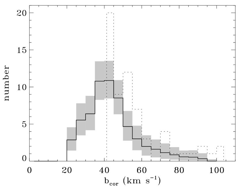
Given the uncertain relationship between $b_{\rm obs}$ and $b_{\rm T}$ for any given absorber, we apply a statistical procedure to better ascertain thermal line widths. First, we assume that $b_{\rm COG}=b_{\rm T}$ where available. For the remainder, we perform a Monte-Carlo simulation, correcting each observed Probable and Possible BLA linewidth as follows. Each candidate is “corrected” using a randomly selected $b_{\rm COG}/b_{\rm LW}$ ratio from the 138 absorbers in DS08 with well-determined $b_{\rm COG}$ (Fig. 2). Each BLA candidate is simulated $10^{4}$ times and the resulting distribution of $b_{\rm cor}$ is shown in shown in Fig. 8. The survival fraction of an individual BLA candidate (i.e., $b_{\rm cor}\geq 40$ km s^-1) is ($62\pm 5$)% although this includes seven $b_{\rm COG}\geq 40$ km s^-1 absorbers which are not corrected. Roughly 50% of the non-COG BLA candidates survive the correction process.

The corrected linewidths are used to calculate $\Omega_{\rm BLA}$ for each Monte-Carlo simulation. The gas temperature is assumed to be $T=60\,b_{\rm cor}^{2}$ K ($b$ in km s^-1). Neutral fraction as a function of temperature $f_{\rm HI}(T)$ is determined from a CLOUDY simulation as discussed above, and the total hydrogen column density is calculated $N_{\rm H}=N_{\rm HI}/f_{\rm HI}$ for each absorber. Summing over all BLAs, we derive $\Omega_{\rm BLA}$ according to equation (8). The full $\Omega_{\rm BLA}$ distribution for $10^{4}$ simulations (Fig. 9) shows a median and $\pm 1\sigma$ value of of $\Omega_{\rm BLA}=6.3^{+1.1}_{-0.8}\times 10^{-3}\,h_{70}^{-1}$ or a baryon fraction of $\Omega_{\rm BLA}/\Omega_{b}=14^{+3}_{-2}$%. Varying some of these assumptions changes $\Omega_{\rm BLA}$ as discussed below.

4.1.1 Systematic Uncertainties and Trends in $\Omega_{\rm BLA}$

There are a number of uncertainties and assumptions present in our $\Omega_{\rm BLA}$ determination which can affect $\Omega_{\rm BLA}$ in several ways. Since we are inferring a total hydrogen column density from an observed neutral trace component, both $b$-values and $N_{\rm HI}$ have a very large lever arm with which to act on the total baryon count.

First, we assume that the COG-determined (or statistically corrected) line width is entirely due to thermal broadening. As discussed above, even a noise-free COG can overestimate a true line width by $20-50$% in the case of undetected, blended components. If we assume all $b_{\rm COG}$ values overestimate $b_{\rm T}$ by 20% (as discussed in Section 2.1), the post-correction survival fraction of BLAs becomes much lower ($34\pm 4$%) and $\Omega_{\rm BLA}=(2.4^{+0.6}_{-0.4})\times 10^{-3}$, more than a factor of two lower than our assumed $b_{\rm COG}=b_{\rm T}$ value.

Second, since IGM absorbers are thought to be quite large in extent and generally unvirialized, there is potentially a Hubble expansion between one side of the cloud and another. Using a typical absorber scale of 350 kpc (Danforth et al., 2006; Danforth & Shull, 2008), we might expect a differential $\Delta v\sim 24\,h_{70}$ km s^-1 between the two sides. This would add in quadrature with the other non-thermal line-broadening effects. Running the simulation with this additional non-thermal correction in place yields a lower mass fraction from BLAs: $\Omega_{\rm BLA}=3.7^{+1.0}_{-0.7}\times 10^{-3}$.

Third, it is unknown how many of our perceived broad lines have a narrow component to them, and conversely, how many blended Ly$\alpha$ forest lines contain a weak, broad component dominated by a narrow absorber. The BLA column density is overestimated for the former lines and uncounted for the latter. Future observations with high S/N ($\gtrsim 30$) from the Cosmic Origins Spectrograph may disentangle some of these lines, but many blended, multiphase systems will likely remain permanently entangled (see Fig. 3), leaving the final BLA baryon census uncertain.

We assume that the detectability of a line of a particular width/depth is a function purely of the local signal-to-noise ratio of the data. Based on this assumption, the data are not less than 80% complete for the range of BLA candidates. If this assumption is optimistic and the data is actually incomplete to $\sim 50\%$ in some cases, the numerator in Eq. 8 may rise by as much as $\sim 60\%$ for some absorbers in the sample. The contribution to $\Omega_{\rm BLA}$ from these terms would increase accordingly, but we expect the correction to the total $\Omega_{\rm BLA}$ sum to be minor.

In this work, we have considered only absorbers with $b_{\rm LW}\geq 40$ km s^-1. However, the distribution of $b_{\rm LW}/b_{\rm COG}$ values (Figure 2) shows that 12% (20/164 COG solutions) have $b_{\rm LW}/b_{\rm COG}<1$. Correcting narrow lines by ratios less than unity will result in a statistical line broadening and could, in principle, create additional BLA candidates. A closer look at the data suggests that “scatter-up” is a small effect. The smallest $b$-ratio in the DS08 distribution is $b_{\rm LW}/b_{\rm COG}\sim 0.7$, so only absorbers with $28\leq b_{\rm LW}<40$ km s^-1 would be broadened to $b_{\rm cor}\geq 40$ km s^-1. There are 82 Ly$\alpha$ absorbers in DS08 in the seven sight lines examined here. On average, a maximum of $82\times 0.12\approx 10$ absorbers would be scattered up. However, due to the opposing trends in $b_{\rm LW}$ and $b_{\rm LW}/b_{\rm COG}$ distributions, the likely number is smaller ($4-5$). Additionally, we have not scrutinized the full sample of $30\leq b_{\rm LW}<40$ km s^-1 absorbers for obvious multiple component structure, which can only reduce the likely number of additional BLAs. Thus, we expect these “scattered-up” narrow lines to be a small correction to $\Omega_{\rm BLA}$.

4.2. Comparison to Previous Work

Previous BLA studies have approached the issues of line identification, line width, and $f_{\rm HI}$ in different ways and most have used some or all of the same datasets studied here. It is instructive to look at the assumptions in and results from these studies to see how different systematics affect $d{\cal N}/dz$ and $\Omega_{\rm BLA}$. All of these values are shown in Fig. 9 in comparison to our results.

Richter et al. (2004) study $\sim 9$ BLAs in the PG 1259$+$593 sight line. They find $(d{\cal N}/dz)_{\rm BLA}\approx 23$ and calculate $f_{\rm HI}$ in CIE from inferred temperature. They note that $b_{\rm LW}$ overestimates $b_{\rm T}$ and thus quote only an upper limit $\Omega_{\rm BLA}\leq 3.3\times 10^{-3}\,h_{70}^{-1}$, roughly half of our result. However, this is a single sight line and the difference may be explainable by cosmic variance.

Figure 10.— Examples of four Possible BLAs toward PKS 0405$-$123 measured in STIS/E140M data which can either be confirmed or refuted based on $S/N\approx 50$ COS/G130M Early Release Observations. The bottom spectra in each panel show the STIS/E140M data used in our analysis to derive consensus $N$ and $b$ values (listed). The upper spectra are COS data with prominent lines labeled and offset upward by 1.5. Panel (a) shows a BLA candidate which has essentially the same profile in both datasets. Panels (b) and (c) show absorbers which show a significantly different structure in the high-S/N COS data. Panel (d) shows a reported Possible BLA which does not appear in the COS spectrum. All data are smoothed to their respective resolution elements. The consensus line fit of the STIS data is marked by a dashed line in both profiles.

Richter et al. (2006) analyze H 1821$+$643 and PG 0953$+$415 and bring in the results from PG 1259$+$593 (Richter et al., 2004) and PG 1116$+$215 (Sembach et al., 2004). They find 20 and 49 BLAs in their “secure” and total samples, with $(d{\cal N}/dz)_{\rm BLA}=22$ and $(d{\cal N}/dz)_{\rm BLA}=53$, respectively. Assuming CIE, they find $\Omega_{\rm BLA}>2.7\times 10^{-3}\,(3.8\times 10^{-3})\,h_{70}^{-1}$, but the value becomes unphysically large ($>\Omega_{b}$) if CIE $+$ photoionization is assumed (dashed curve in Figure 1).

Lehner et al. (2007) compile data from seven sight lines including four from previous work (PG 1259$+$593 (Richter et al., 2004), HE 0226$-$4110 (Lehner et al., 2006), HS 0624$+$6907 (Aracil et al., 2006b) and PG 1116$+$215 (Sembach et al., 2004)), two from as-yet-unpublished private communication (PG 0953$+$415, Tripp et al. in prep. and H 1821$+$643, Sembach et al. in prep), a detailed reanalysis of PKS 0405$-$123. They perform quality and column-density cuts on 341 Ly$\alpha$ lines and end up with $\sim 60$ BLAs for a density $(d{\cal N}/dz)_{\rm BLA}=30\pm 4$. To deal with blended components and non-thermal broadening, L07 randomly eliminate 1/3 of their BLAs with $40<b<65$ km s^-1 (all absorbers with $b>65$ km s^-1 are kept). Nonthermal broadening is assumed to be $\sim 10$% of the total line width (Richter, Fang, & Bryan, 2006), so temperatures are calculated assuming $b_{\rm T}\approx 0.9\,b_{\rm obs}$. They calculate $\Omega_{\rm BLA}$ assuming both CIE and Richter’s CIE $+$ photoionization parametrization and find $\Omega_{\rm BLA}=3.6\times 10^{-3}\,h_{70}^{-1}$ and $9.1\times 10^{-3}\,h_{70}^{-1}$, respectively or $\Omega_{\rm BLA}/\Omega_{b}=8\%$ and $20\%$, for each case.

At higher redshift, Prause et al. (2007) observed BLAs in the spectra of five $1.34<z<1.94$ AGN using both the near-UV STIS/E230M grating on HST and the ground-based UV Echelle Spectrograph at the ESO Very Large Telescope. In total, they found 9 good BLA candidates and an additional 29 tentative cases in the redshift range $0.9\lesssim z\lesssim 1.9$. They derive a value of $\Omega_{\rm BLA}=(2.2\pm 0.1)\times 10^{-3}\,h_{70}^{-1}$ for the 9 good BLA candidates and $\Omega_{\rm BLA}=(14\pm 2)\times 10^{-3}\,h_{70}^{-1}$ for the entire sample.

4.2.1 Broad Absorbers in Cosmic Origins Spectrograph Observations

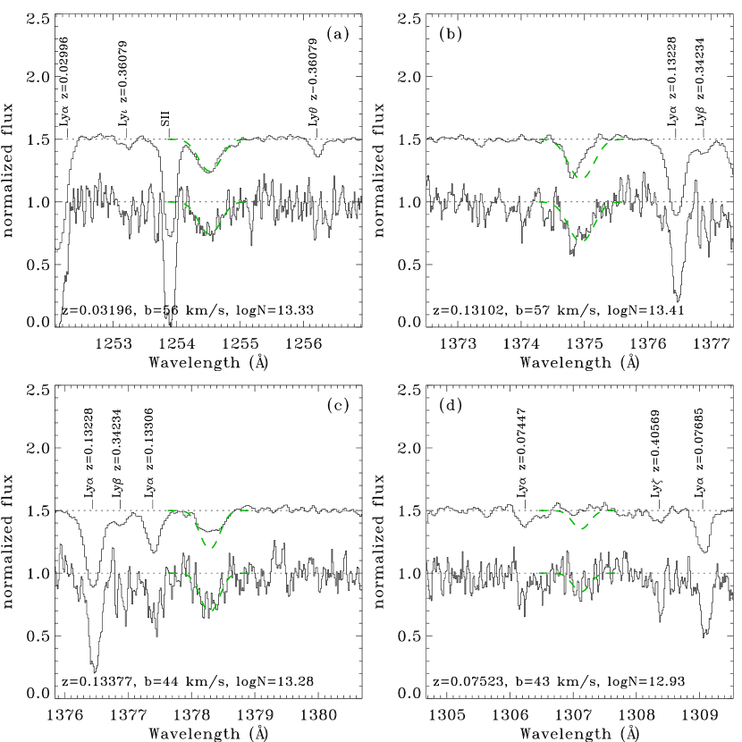
Late in the analysis process, we obtained observations of PKS 0405$-$123 by the HST/Cosmic Origins Spectrograph (Green et al., 2010; Osterman et al., 2010) as part of its public Early Release Observations (ERO) program. These data were obtained in the G130M grating ($\rm 1132~{}\AA<\lambda<1468~{}\AA$) with a nominal resolution $R\sim 20,000$ ($\Delta v=15$ km s^-1). Seven orbits in total ($\sim 17$ ksec) were devoted to ERO observations, with three taken prior to when an accurate focal alignment was achieved and four afterward. A close examination of the data shows no difference in line profiles for any of the ISM or IGM lines of interest, so observations from all seven orbits were aligned and coadded.

The resulting spectrum is of exquisite quality with $S/N\geq 40$ per nominal seven-pixel resolution element at most locations. Owing to the differences in detector technology and the different grating positions used in the observations, the COS data are free of much of the fixed-pattern noise that plagues the corresponding STIS/E140M observations. This, coupled with the very high S/N, makes COS ideal for verifying the BLA candidates discussed in this paper.

Eighteen of the BLA candidates toward PKS 0405$-$123 measured in STIS/E140M data are also covered in the COS observations. Five of these cases are blended components of strong absorption systems, which are difficult to confirm or refute, but the COS data is consistent with the STIS observations. Of the 13 weaker absorption lines, seven show a good match between STIS and COS data. However the STIS-measured line profile is substantially different in four cases and missing altogether in another three. Figure 10 shows several examples where BLA candidates can be either confirmed or refuted based on COS observations.

This is a good demonstration of the importance of fully understanding the instrumental effects of a particular spectrograph. While the COS data are not free of fixed pattern noise, it is independent of that in the STIS observations. Furthermore, it is evidence that the $\sim 10\times$ sensitivity increase of COS over STIS will revolutionize the study broad Ly$\alpha$ absorbers, both through higher S/N and sensitivity to numerous, fainter targets. Since this work relies on a uniform analysis of consistent datasets by independent groups, we do not change any of our BLA designations in light of new, higher-quality data from COS. However, we note the results of our COS absorber verification where possible in the individual absorber comments in the Appendix.

5. Conclusions and Summary

Broad Ly$\alpha$ absorbers are a potentially powerful method of measuring the extent and distribution of gas at $T\geq 10^{5}$ K in the intergalactic medium without relying on metal enrichment. The small hydrogen neutral fraction even at WHIM temperatures will result in broad, shallow H I profiles that can be translated into temperatures and total hydrogen column densities. Unfortunately, BLAs present some observational challenges and ambiguities. Broad, shallow absorbers are difficult to detect in data of only moderate S/N and in multi-phase systems. Detected BLAs are strongly biased toward cooler temperatures where lines are relatively narrower and the neutral fraction is higher. Furthermore, identification of bona fide BLAs relies crucially on the line component structure, knowledge of instrumental features and an accurate continuum definition.

We attempt to work around these problems by independent reduction and analysis of seven AGN sight lines containing 119 purported broad Ly$\alpha$ lines reported in the literature (mainly DS08 and L07 and sources therein). We assign consensus values for column density and line width based on two independent analyses by two different research groups. The purported BLAs are split into three qualitative categories based on the consensus linewidth, detailed analysis of the absorption profile, and other factors. Probable BLAs (15 systems) are those showing $b_{\rm LW}>60$ km s^-1 and no obvious asymmetry or component structure. Systems with curve-of-growth determined linewidths $b_{\rm COG}>40$ km s^-1 are also deemed Probable BLAs. Possible BLAs (48 systems) are those with $40<b_{\rm LW}<60$ km s^-1, those absorbers with potential component structure or asymmetries, or some plausible reason to doubt their identity as BLAs. The remaining systems (56) are ruled out as being BLAs for a number of reasons: alternate line identification, $b_{\rm LW}<40$ km s^-1, probable component structure, or simply failing to appear in our reduction of the data.

Taking all of the probable BLAs and $50\pm 50$% of the possible category, we see $39\pm 24$ BLAs along a total redshift pathlength $\Delta z=2.193$ ($\Delta X_{\rm tot}=1.773$) in the seven AGN sight lines surveyed. This gives a detection frequency of $d{\cal N}/dz_{\rm BLA}=18\pm 11$ ($d{\cal N}/dX_{\rm BLA}=22\pm 14$). This frequency is similar to that of O VI, another potential WHIM tracer with $(d{\cal N}/dz)_{\rm OVI}=15\pm 3$ (Danforth & Shull, 2008; Tripp et al., 2008), though the BLA frequency has considerably greater uncertainty. Indeed, while the detection or non-detection of highly ionized ions (O VI, N V, Ne VIII, etc) was not taken into account in our BLA categorization, 40% of the probable BLAs and 20% of the combined probable-plus-possible samples show reasonable O VI detections. The incidence of O VI detections in narrow Ly$\alpha$ lines is $\sim 15$%.

The relationship of WHIM to galaxies is another key area of interest. It is likely that small galaxies with weak gravitational fields are important for IGM heating and enrichment (e.g., Stocke et al., 2004). Unfortunately, surveys for low-luminosity galaxies tend to be unreliable at redshifts greater than a few hundredths. However, we found eight BLAs in regions of fairly complete galaxy surveys ($L\gtrsim 0.2\,L^{*}$) that provide nearest-galaxy distances of 60 kpc out to nearly 3 Mpc. The detection of O VI in conjunction with broad Ly$\alpha$ was highly correlated with galaxy distance as the four BLAs with $d\lesssim 600$ kpc showed O VI detections at some level, while the four BLAs at $d\gtrsim 600$ kpc appear to be free of O VI absorption. This result gives significant support for BLAs probing gas that O VI surveys do not detect. Using the above O VI detection statistics, our BLAs suggest that $\sim 80$% of the baryons are not already accounted for in O VI surveys.

A main and crucial uncertainty in BLA surveys is disentangling thermal and non-thermal line broadening, as measured line width overpredicts the thermal linewidth, often by an unknown amount. Previous studies have recognized this phenomenon and dealt with it in a variety of ways, including arbitrarily throwing out some fraction of measured BLAs from a sample or scaling measured line widths by some uniform factor. We approach the problem by looking at curve-of-growth $b$-values ($b_{\rm COG}$): the doppler b-parameter measured from a single line (typically Ly$\alpha$) overpredicts that from a full COG analysis (Danforth et al., 2006) by a factor of $\sim 1.5\pm 0.9$ (though we also show how even a COG can overpredict the true linewidth). Since most broad Ly$\alpha$ systems are fairly weak, confirmation in higher-order Lyman lines is usually not possible. Instead, we statistically correct for the single-line $b$-value overprediction based on the observed $b_{\rm LW}/b_{\rm COG}$ distribution in DS08. We find in our simulations that $55\pm 5$% of the reported BLAs survive the correction process with $b_{\rm cor}\geq 40$ km s^-1, corresponding to $T\geq 10^{5}$ K.

From temperatures derived from line widths, we can estimate the neutral fraction of a particular absorber and hence the total hydrogen column associated with a particular H I detection. The total amount of gas at $T>10^{5}$ K traced by these BLAs can then be estimated as a fraction of the closure density of the Universe. We use a Monte-Carlo simulation to statistically correct the observed BLA linewidths. Our median value of $\Omega_{\rm BLA}=6.3^{+1.1}_{-0.8}\times 10^{-3}\,h_{70}^{-1}$ ($\Omega_{\rm BLA}/\Omega_{b}=14^{+3}_{-2}$%) based on $10^{4}$ Monte-Carlo simulations of each BLA. Since $\sim 80$% of these BLA baryons are not in O VI systems, the combination of O VI $+$ BLA WHIM searches can account for $\Omega_{\rm WHIM}/\Omega_{b}\sim 20\%$. This includes $\sim 8$% from O VI (DS08) and an additional $\sim 12$% in metal-poor BLAs. It is clear that systematic uncertainties involved in BLA surveys are comparable to or larger than the statistical fluctuations from cosmic variance among the sight lines, and more work must be done to understand the individual systems.

To illustrate the importance of methodology and individual systems to the baryon census, we compare our result to that of L07. L07 used the same set of AGN sight lines used here and a more inclusive set of BLA candidates. They assume $b_{\rm T}=0.9b_{\rm LW}$ as in Richter, Fang, & Bryan (2006), calculated hydrogen neutral fraction via a CIE assumption (very similar to the CLOUDY $\log\,N=-2$ model used here), and randomly eliminated 1/3 of the $40<b<65$ km s^-1 absorbers which gave a result of $\Omega_{\rm BLA}=3.6\times 10^{-3}\,h_{70}^{-1}$ or $\Omega_{\rm BLA}/\Omega_{b}=8\%$ or $\sim 60$% of our value. If, instead, $f_{\rm HI}$ is based on the CIE $+$ photoionization model of Richter, Fang, & Bryan (2006), the L07 value rises to $\Omega_{\rm BLA}=9.1\times 10^{-3}\,h_{70}^{-1}$, or $\sim 40$% larger than our result (see Fig 9).

Future observations of low-redshift BLA systems with the Hubble Space Telescope/Cosmic Origins Spectrograph (COS) will improve the BLA census in several important areas. First, five of the seven sight lines studied here (HE 0226$-$4110, PG 1116$+$215, PKS 0405$-$123, PG 0953$+$415, and PG 1259$+$593), as well as over a dozen other AGN sight lines observed with STIS/E140M will be observed by COS as part of the Guaranteed Time Observations. Some of the scheduled GTO observations are high-S/N spectra of BL Lac objects chosen specifically to search for BLAs against non-thermal power-law continua. More AGN observations are scheduled in several large HST Cycle 17 Guest Investigator programs (PIs: Tripp, Tumlinson). Observations of the same targets by different instruments will help sort out real BLAs from instrumental features. Furthermore, the exquisite S/N expected from COS data, both for previously observed and new sight lines, will be crucial in determining line profiles, identifying blended systems, and finding the expected population of weak, broad systems. Late in our analysis process, we obtained high-S/N COS/G130M observations of PKS 0405$-$123 which shed considerable light on individual BLA candidates. We discuss this further and show several examples of possible BLAs observed with much higher S/N in the Appendix. While some BLA Candidates are confirmed by the COS data, there are some significant differences which suggest that the actual number of BLAss less than catalogued herein. Finally, the high sensitivity of COS compared with STIS will allow a much larger pathlength of the low-$z$ IGM to be surveyed, increasing our statistics on intergalactic absorbers ranging from metal-line systems to BLAs. Increases in both the O VI and BLA catalogs will undoubtedly occur. It will be very interesting to see where the WHIM baryon census stands ten years hence.

We wish to acknowledge the great assistance rendered by Steve Penton in performing custom reductions of the STIS/E140M data and investigating the mysterious differences between reported reductions. Similarly, Brian Keeney performed the nearest-galaxy searches. Teresa Ross was instrumental in tracking down discrepancies between published line lists. This work was supported by the COS GTO grant NNX08-AC14G from NASA, HST Archive grant AR-11773.01-A from STScI, NSF Theory grant AST07-07474, and NASA Theory grant NNX07-AG77G.

Appendix A Notes on Individual Absorbers

We present here more detailed comments on individual BLA candidates than is present in Table 2. Each system is identified by sight line, redshift, and our BLA classification (A=Probable BLA, B=Possible BLA, C=not a BLA). We add a fourth category here (X) for narrow Ly$\alpha$ systems which are adjacent to or blended with BLA candidates. See Table 2

A.1. HE 0223$-$4110

$z=0.06083$ (B):

Strong line detected in Ly$\alpha$,$\beta$ ($W_{\rm Ly\alpha}=557\pm 20$ mÅ, $W_{\rm Ly\beta}=313\pm 113$ mÅ) with suggestion of broad wing on blue side and possible component structure. No metal lines to clarify component structure. COG for full system gives $b_{\rm COG}\sim 36$ km s^-1 with large uncertainties. We list this as a possible BLA since there the broad wing on the blue side suggests a broad component.

$z=0.16339$ (B):

Very strong Ly$\alpha$ system. Ly$\beta$ is blended with Galactic Si II absorption, but appears narrow. Ly$\gamma$ absorption is present but weak. COG solution doesn’t converge and there are signs of multiple components. No metal lines to illustrate component structure.

$z=0.20700$ (B):

Saturated, broad Ly$\alpha$ profile with possible weak, broad component seen in the wings. Ly$\beta$,$\gamma$ show asymetric profiles. Strong O VI, C III, Si III (DS08) and Ne VIII (Savage et al., 2005) detections as well as possible S IV. We adopt the Savage et al. (2005) measurements for the BLA component, but list the system only as a possible BLA since the component structure is ambiguous.

$z=0.30930$ (B):

Strong, broad system with probable component structure in Ly$\alpha$,$\beta$,$\gamma$: $W_{\rm Ly\alpha}=388\pm 7$ mÅ, $W_{\rm Ly\beta}=130\pm 3$ mÅ, $W_{\rm Ly\gamma}=33\pm 3$ mÅ. Multi-valued COG solution: $b_{\rm COG}=34\pm 2$ km s^-1 ($\alpha,\beta$) or $b_{\rm COG}=44\pm 6$ km s^-1 ($\alpha,\gamma$). Due to this ambiguity and the likely component structure, we list this as a possible BLA. No metal lines.

$z=0.38420$ (C):

Strong system with ambiguous component structure in Ly$\alpha$. However, Ly$\beta$ profile shows two clear components. Two or three components seen in Ly$\beta$ profile despite poor S/N. COG on stronger, red, component gives $b_{\rm COG}\sim 31$ km s^-1.

$z=0.39641$ (B), $z=0.39890$ (B), $z=0.40034$ (B):

Possible continuum ripples shown in Figure 5 and discussed in the text. In particular, a very similar feature appears in the data at 1702.5Å in the PG 0953$+$414 data at $z_{\rm abs}>z_{\rm AGN}$ which looks similar to the $z=0.40034$ feature toward HE 0223$-$4110, however other spectra at higher S/N do not show this feature.

A.2. PKS 0405$-$123

$z=0.03196$ (B):

Broad Ly$\alpha$ profile ($W_{\rm Ly\alpha}=108\pm 22$ mÅ, $b_{\rm LW}=57\pm 8$ km s^-1), but weak, narrow Ly$\beta$ ($W_{\rm Ly\beta}=50\pm 6$ mÅ, $b_{\rm LW}=35\pm 4$ km s^-1). COG is poorly constrained: $b_{\rm COG}>10$ km s^-1. Possible BLA based on Ly$\alpha$ alone. COS observations are consistent with the STIS/E140M data.

$z=0.05896$ (C):

Noisy data suggests two weak, narrow components each with $b\sim 20$ km s^-1. COS spectrum confirms the two components with $b_{\rm LW}=23$ and 27 km s^-1 are not BLAs.

$z=0.07218$ (C):

Very marginal feature which is not clearly Ly$\alpha$. Identified as C III $z=0.3340$ by DS08. Absorption feature confirmed in COS data as real with $b_{\rm LW}=30\pm 3$ km s^-1.

$z=0.07523$ (B):

Very weak detection measured by both W06 ($b_{\rm LW}=56$ km s^-1) and L07 ($b_{\rm LW}=48\pm 20$ km s^-1). High-S/N COS observations show no absorption at this position ($W<11$ mÅ).

$z=0.08139$ (A):

Moderately strong system with $b_{\rm LW}\sim 53$ km s^-1, $W_{\rm Ly\alpha}=261\pm 16$ mÅ. Ly$\beta$ shows $W=90\pm 8$ mÅ but is blended with Ly$\epsilon$ $z=0.18269$ ($W_{\rm Ly\alpha}\sim 670$ mÅ). If this entire absorption feature is taken as Ly$\beta$ $z=0.08139$, then $b_{\rm COG}>22$ km s^-1. However, if only part of absorption is taken as Ly$\beta$ ($W_{\rm Ly\beta}\sim 45\pm 10$ mÅ), the COG linewidth is large but uncertain: $b_{\rm COG}=74\pm 30$ km s^-1. Given this ambiguity and the broad, clean Ly$\alpha$ profile, we list the absorber as a probable BLA.

$z=0.09659$ (B):

Strong Ly$\alpha$ system ($W_{\rm Ly\alpha}\sim 500$ mÅ) with excess in blue wing indicating possible broad component. DS08 find $b_{\rm COG}=36\pm 4$ km s^-1 and W06 find $b_{\rm LW}=37\pm 1$ km s^-1 for the entire system. However, L07 fit a broad component to the system and we take this as a possible BLA due to the ambiguous nature of the fit. DS08 report O VI detected in both lines of the doublet associated with the system, though it is unclear to which component it may correspond. COS observations show consistent line profile, but BLA component cannot be verified.

$z=0.10298$ (C):

Very marginal feature which is not obviously a single absorber. W06 measure $b_{\rm LW}=60\pm 14$ km s^-1. COS data shows a clear blend of two absorbers $b_{\rm LW}=27\pm 5$ and $42\pm 3$ km s^-1, thus no BLA is confirmed in this system..

$z=0.10419$ (C):

Very marginal detection not confirmed by DS08. COS observations show no absorption at this position ($W<10$ mÅ).

$z=0.13102$ (B):

Moderate absorption feature with broad wing on red edge suggesting possible BLA component. COS observations show absorption at this wavelength ($b_{\rm LW}=35\pm 1$ km s^-1, $\log\,N=13.18\pm 0.01$), significantly narrower than that observed by STIS.

$z=0.13377$ (B):

Noisy data with moderately broad absorption. COS observations show a clear absorber at this location ($b_{\rm LW}=53\pm 2$ km s^-1, $\log\,N=13.10\pm 0.02$) but significantly shallower and broader than the STIS profile.

$z=0.13646$ (C):

Marginal line with likely components. Single-component fit from W06 gives $b_{\rm LW}=49\pm 8$ km s^-1. COS confirms double component structure, $b_{\rm LW}=23\pm 4,26\pm 2$ km s^-1.

$z=0.13924$ (C):

No detection in L07. Marginal feature in DS08 and W06. Not clearly a single component even if real. COS observations show two absorbers offset in velocity, but nothing corresponding to the reported line profile.

$z=0.15304$ (C):

Strong, broad line ($W_{\rm Ly\alpha}=263\pm 10$ mÅ) identified as Ly$\alpha$ by L07, but corresponding Ly$\beta$ nondetection ($W_{\rm Ly\beta}<24$ mÅ) is inconsistent with a single Ly$\alpha$ absorber. Unknown line identification. COS confirms line profile.

$z=0.16121$ (C):

Strong absorber with several clear components. Strong metal lines likely make up the flanking components leaving little room for a broad Ly$\alpha$ core. COS confirms general profile. Thus COS does not confirm this BLA.

$z=0.16678$ (B) and $z=0.16714$ (C):

Strong Ly$\alpha$ complex ($W_{\rm Ly\alpha}\sim 650$ mÅ) with an asymmetry on the blue wing. Line can be fit with broad a broad and narrow component, but decomposition is suspect. Ly$\beta$ ($W_{\rm Ly\beta}\sim 450$ mÅ) shows no sign of the broad, blue component. Strong system ($z=0.16714$) shows obvious component structure in various metal lines. The system shows strong O VI and N V absorption (DS08), but it is unclear with which component it is associated. COS observations show a consistent line profile, but cannot confirm or deny the presence of a BLA component.

$z=0.17876$ (B):

Asymmetric Ly$\alpha$ line with very marginal Ly$\beta$ detection. COG analysis by DS08 gives $b_{\rm COG}=18^{+44}_{-7}$ km s^-1. Apparent Optical Depth (AOD) line fits to Ly$\alpha$ line gives much broader profile ($b_{\rm LW}\sim 60$ km s^-1; W06 measures $b_{\rm LW}=58\pm 6$ km s^-1). Well fit by an offset broad+narrow pair ($b_{\rm LW}=57$, 14 km s^-1), but inconclusive. We take the AOD measurements as concensus in this case. COS observations confirm the general profile shape of this absorber and consistent line measurements.

$z=0.18269$ (B):

Strong H I system ($W_{\rm Ly\alpha}\sim 690$ mÅ) with at least two components, possibly more. Ly$\beta$ is blended with Galactic Ly$\alpha$. Ly$\gamma$ shows strong, moderately asymmetric profile ($W_{\rm Ly\gamma}=139\pm 11$ mÅ). COG gives $b_{\rm COG}=49^{+11}_{-7}$ km s^-1, but probable component structure relegates this to a possible BLA. System shows several O VI components. COS observations confirm the line profile of this strong absorber, but cannot confirm or deny the presence of a BLA.

$z=0.19086$ (B):

Weak, noisy absorber with possible component structure. COS observations do not show an absorption line at this position ($W_{r}<22$ mÅ).

The COS ERO spectral coverage ($1132<\lambda<1468$) ends at this maximum redshift.

$z=0.24513$ (B) and $z=0.24553$ (X):

Pair of well-separated Ly$\alpha$ absorbers. System at $z=0.24513$ appears narrow ($b_{\rm LW}=30\pm 5$ km s^-1) but both L07 and W06 measure $b\approx 55$ km s^-1. We adopt a consensus $b$ and $N$ intermediate between the two measurements to account for possible continuum and reduction differences.

$z=0.32500$ (C):

Marginal detection, however there is a correlation between features in Ly$\alpha$,$\beta$. Probably multiple components. DS08 report $b_{\rm COG}=21$ km s^-1, however we find this to be more reasonable as a lower limit and the COG solution doesn’t fit the absorption profile very well. W06 report $b_{\rm LW}=81\pm 11$ km s^-1. Higher S/N data on this absorber should prove interesting. Given the marginal nature of this feature and the likely component structure, we list it as a non-BLA.

$z=0.35092$ (B), $z=0.35149$ (X):

Strong Ly$\alpha$ system flanked by Si III $z=0.36079$ and Ly$\alpha$ $z=0.35149$. Ly$\alpha$,$\beta$ curve of growth gives $b_{\rm COG}=56\pm 15$ km s^-1 (DS08), but Ly$\alpha$,$\gamma$ curve of growth gives $b_{\rm COG}=27\pm 5$ and seems to better match the profile. W06 and L07 measure $b_{\rm Ly\alpha}=38\pm 2$ km s^-1 and $b_{\rm Ly\alpha}=40\pm 8$ km s^-1, respectively. Both Ly$\alpha$ and Ly$\beta$ show asymmetric profiles suggesting multiple components. We accept the Ly$\alpha$ measurements as consensus in this case and list the system as a possible BLA.

$z=0.36150$ (C) and $z=0.36079$ (X):

Strong, blended Ly$\alpha$ systems with an ambiguous component structure and noisy data. Two-component fit gives $b_{\rm LW}=75\pm 10$, $39\pm 5$ km s^-1 for the $z=0.36150$ and $z=0.36079$ components, respectively. The $z=0.36150$ component, however, doesn’t appear in Ly$\beta$ ($W_{\rm Ly\beta}\leq 9$ mÅ); based on the Ly$\alpha$ component, the expected Ly$\beta$ line should be $W_{\rm Ly\beta}\sim 50$ mÅ. Meanwhile, a Ly$\beta$,$\gamma$ curve of growth fit to the the $z=0.36079$ component (ignoring the noisy, possibly blended Ly$\alpha$ profile) gives $b_{\rm COG}=25\pm 3$ km s^-1, $\log\,N=15.18\pm 0.13$ cm^-2. We conclude that neither system is a BLA.

$z=0.40886$ (B):

Strong Ly$\alpha$ system ($W_{\rm Ly\alpha}=430\pm 10$ mÅ) at the long-wavelength, noisy end of the STIS/E140M range. Ly$\beta$,$\gamma$ also present ($W_{\rm Ly\beta}=126\pm 15$ mÅ, $W_{\rm Ly\gamma}=68\pm 10$ mÅ), both with asymmetric profiles. Ly$\alpha$,$\beta$ and Ly$\alpha$,$\gamma$ COG solutions inconsistent but generally $b_{\rm COG}\sim 40$ km s^-1. Possible BLA, but probable component structure.

A.3. HS 0624$+$6907

$z=0.04116$ (C):

Weak feature consistent with Si III $z=0.06346$, a system in which many other ionic lines are also detected.

$z=0.05437$ (B), $z=0.05515$ (B), and $z=0.05484$ (C):

Strong Ly$\alpha$ system ($W_{\rm Ly\alpha}\sim 450$ mÅ) with several plausible BLA subcomponents. The $z=0.05437$ line appears as a very marginal, noisy absorption on the blue wing while the $z=0.05515$ component is an excess on the red side of the main absorption line. The strong central component at $z=0.05484$ is fit well by a $b_{\rm LW}\sim 35$ km s^-1 component despite the $b_{\rm COG}=45^{+25}_{-9}$ km s^-1 value reported in DS08. The narrow feature at 1283.15 Å can be unambiguously identified as Si III $z=0.0635$. The BLA nature of these lines relies on the details of the component structure which is quite ambiguous and difficult to disentangle.

$z=0.06346$ (C):

Strong Ly$\alpha$ system with measured $b_{\rm LW}>40$ km s^-1 but $b_{\rm COG}<40$ km s^-1 with O VI detected in both lines of the doublet (DS08). H I profile looks symetric, but there are two clear components in Si IV, C IV, Si III, and S III.

$z=0.13597$ (B):

Weak double profile. Feature at 1381.4Å is Ly$\beta$ $z=0.3468$ but broader feature at 1381.0Å is a plausible BLA with low-significance O VI detections at both 1032 and 1038Å. Possible BLA based on the measured line though the large error bars and O VI detection could argue for this being a Probable BLA.

$z=0.30994$ (B):

Broad, weak absorption feature identified as Ly$\alpha$ by both L07 and DS08. However considerable continuum uncertainty yields highly incompatible $b,N$ solutions. Possible, low-significance O VI detected as well. In any case, profile is asymmetrical and not obviously a single component.

$z=0.31045$ (C), $z=0.31088$ (C):

Broad, asymmetric features which are not obviously real. Possible continuum differences.

$z=0.31790$ (B):

Moderate, narrow Ly$\alpha$ line with asymmetry on the red wing and good O VI detections in both lines of the doublet. Possible multiphase system and/or continuum fit uncertainties. Possible BLA.

$z=0.32089$ (C):

Strong, moderately-narrow line is a poor fit to DS08 COG solution ($b_{\rm COG}=44^{+13}_{-14}$ km s^-1). Ly$\alpha$ absorption is anomalosly large given observed Ly$\beta$,$\gamma$, however there are no other obvious contributors to the Ly$\alpha$ line strength. We confirm the $b_{\rm LW}=31\pm 1$ km s^-1 solution of L07 for this absorber.

$z=0.33976$ (A):

Strong, broad system with no obvious components and detections in Ly$\alpha$,$\beta$,$\gamma$. Good COG solution gives $b_{\rm COG}=41\pm 6$ km s^-1. O VI detected in both lines of the doublet (DS08).

A.4. PG 0953$+$415

$z=0.04382$ (C):

Reported as O VI $\lambda$1032 at $z=0.22974$ by Tripp et al. (2008). Interestingly, this is a “blind” O VI system with little or no accompanying Ly$\alpha$ absorption ($W_{\rm Ly\alpha}<7$ mÅ).

$z=0.05879$ (B):

Narrow line with a possible excess in line wings suggesting a multiphase system. Very ambiguous decomposition. We take the L07 values as the consensus.

$z=0.12784$ (C):

Claimed broad blue wing on a narrower Ly$\alpha$ system. We see no good evidence for this system in our reduction of the data.

$z=0.17985$ (B):

Weak single or double absorption. Potentially fit as single BLA or two narrow components ($b_{\rm LW}\sim 20$).

$z=0.19126$ (B):

Asymmetric Ly$\alpha$ profile with uncertain decomposition. Formal AOD linewidth is $b_{\rm LW}\approx 66$ km s^-1  however, two components ($b_{\rm LW}=40$, 32 km s^-1) provides a better fit. We adopt $b_{\rm LW}=40:$ km s^-1 and $\log\,N=13.3$ cm^-2 as consensus values.

$z=0.19361$ (C):

Strong narrow Ly$\alpha$ system with very weak Ly$\beta$,$\gamma$ counterparts. DS08 report a Ly$\alpha$,$\beta$ solution ($b_{\rm COG}=24^{+4}_{-3}$ km s^-1, $\log\,N=14.15\pm 0.04$ cm^-2) which is stronger than the data can easily support. We measure $b_{\rm LW}=37\pm 2$ km s^-1 instead and adopt that value here.

A.5. PG 1116$+$215

$z=0.08587$ (B), $z=0.08632$

Pair of very shallow, ripples in the continuum with $b_{\rm LW}\sim 55$ and $b_{\rm LW}\sim 34$ km s^-1, respectively, both with considerable uncertainty. Broader feature is possible BLA.

$z=0.09279$ (A):

Very weak, broad system blended with two weak, narrow features (possible Galactic C I). While profile looks questionable, it is more obvious when looking at a broader wavelength range. Eliminating the two sharp features gives a very plausible BLA.

$z=0.13370$ (A):

BLA with a low-significance O VI $\lambda$1032 detection ($\log\,N_{\rm OVI}\approx 13.2\pm 0.3$ cm^-2). Potentially fit as two components ($\lambda\approx 1378.3,1378.7$) but $b_{\rm LW}\sim 50$ km s^-1 even in this case.

A.6. PG 1259$+$593

$z=0.00229$ (A):

Ly$\alpha$ line appears on the edge of the broad Galactic Ly$\alpha$ trough and Ly$\beta$ is blended with an O I airglow line in FUSE data. Richter et al. (2004) used night-only data to get a good Ly$\beta$ measurement and constrains $b_{\rm COG}=44^{+9}_{-4}$ km s^-1 which we adopt here.

$z=0.04606$ (C):

Very strong system with obvious components in O VI, C IV, Si III, Si IV. Richter et al. (2004) report two H I components, both with $b_{\rm COG}<40$.

$z=0.14852$ (A):

Strong nearly triangular line profile with detections in Ly$\alpha$,$\beta$. Curve of growth consistent with BLA $b_{\rm COG}\approx 57$ km s^-1 though with large errors. $b_{\rm Ly\beta}\sim 36$ km s^-1.

$z=0.19573$ (B), $z=0.19620$ (X):

Double absorption profile. Shallow, blue feature at 1453.6 Å is plausible BLA candidate ($b_{\rm LW}=46\pm 19$ km s^-1) and was reported as a component to the $z=0.1962$ system by Richter et al. (2004). Marginal N V detection.

$z=0.21136$ (C) and $z=0.43569$

Richter et al. (2004) identify the absorption at 1472.6 Å as Ly$\beta$ $z=0.43569$ and high-res FOS spectra confirm Ly$\alpha$ line at this redshift. Absorption at 1242.5 Å where Ly$\beta$ $z=0.21136$ would be expected is blended with Ly$\alpha$ $z=0.02217$ and unrecoverable. Can’t confirm.

A.7. H 1821$+$643

$z=0.11133$ (A), $z=0.11167$ (X):

Double absorber profile with one broad, one narrow system ($b_{\rm LW}=52,31$ km s^-1). L07 measure this as a single system ($b_{\rm LW}=88\pm 14$ km s^-1). One BLA likely present.

$z=0.12147$ (A), $z=0.12117$ (X):

Strong and highly asymmetric absorber. Red wing Ly$\beta$ is hinted at in the data, but at low significance. System shows $b_{\rm COG}>40$ km s^-1, but there are clearly multiple components. Weak O VI absorption is reported in the system (Tripp et al., 2001, 2008; Oegerle et al., 2000) aligned with broad Ly$\alpha$ wing, however, DS08 do not confirm this detection.

$z=0.14754$ (B) and $z=0.14776$ (X):

Blended system of two, easily separable components ($b_{\rm LW}\approx 42,20$ km s^-1). Marginal Ly$\beta$ detection for both components but COG solution is very poorly constrained ($b_{\rm COG}=22^{+\infty}_{-12}$ km s^-1) for the $z=0.14754$ system.

$z=0.21326$ (A):

Strong system with Ly$\alpha$,$\beta$ detections ($b_{\rm COG}=42^{+5}_{-4}$ km s^-1) though with some hint of component structure. Strong O VI detection in both lines of the doublet. The entire absorber may not represent hot gas, but there is probably a BLA component.

$z=0.22480$ (C):

Very strong system ($W_{\rm Ly\alpha}\sim 800$ mÅ) with clear components in higher Lyman lines. O VI detected. Not confirmed by L07, but clearly not a BLA.

$z=0.22616$ (B):

Moderate absorption feature ($W_{\rm Ly\alpha}=150\pm 8$ mÅ) identified as Ly$\alpha$ by L07. However, corresponding Ly$\beta$ non-detection shows $W_{\rm Ly\beta}\leq 10$ mÅ, inconsistent with a single Ly$\alpha$ system. Possible O VI absorption ($\log\,N_{\rm OVI}=13.4\pm 0.1$ cm^-2) in both lines of the doublet offset $\sim+60$ km s^-1 from the purported H I system. Probable multiple components or misidentification.

$z=0.25814$ (B):

Strongly asymmetric profile suggests a multiphase H I system. Profile is reasonably fit by two components: $b_{\rm LW}\approx 56$, 17 km s^-1. Total line shows $W_{\rm Ly\alpha}=141\pm 3$ mÅ and corresponding weak Ly$\beta$ absorption ($W_{\rm Ly\beta}\approx 24$ mÅ) gives a curve-of-growth solution $b_{\rm COG}=30\pm 7$ km s^-1 for the combined system. In light of this, the component fits seem reasonable and we list this as a possible BLA.

$z=0.26658$ (A):

Strong system with O VI detected in both lines of the doublet. Poorly-constrained COG gives $b_{\rm COG}=68\pm 30$ km s^-1. Individual lines show $b_{\rm LW}=46$ km s^-1 and $b_{\rm LW}\sim 40$ km s^-1. Probable BLA despite poorly-constrained COG.

References

- Aracil et al. (2006a) Aracil, B., Tripp, T. M., Bowen, D. V., Prochaska, J. X., Chen, H.-W., & Frye, B. L. 2006a, MNRAS, 367, 139
- Aracil et al. (2006b) Aracil, B., Tripp, T. M., Bowen, D. V., Prochaska, J. X., Chen, H.-W., & Frye, B. L. 2006b, MNRAS, 372, 959
- Asplund et al. (2005) Asplund, M., Grevesse, N., & Sauval, A. J. 2005, in Cosmic Abundances as Records of Stellar Evolution and Nucleosynthesis, ASP Conf. Ser. 336, 25
- Bregman (2007) Bregman, J. N. 2007, ARA&A, 45, 221
- Cen & Fang (2006) Cen, R., & Fang, T. 2006, ApJ, 650, 573
- Cen & Ostriker (1999) Cen, R., & Ostriker, J. P. 1999, ApJ, 514, 1
- Cen & Ostriker (2006) Cen, R., & Ostriker, J. P. 2006, ApJ, 650, 560
- Danforth & Shull (2005) Danforth, C. W., & Shull, J. M. 2005, ApJ, 624, 555
- Danforth et al. (2006) Danforth, C. W., Shull, J. M., Rosenberg, J. L., & Stocke, J. T. 2006, ApJ, 640, 205
- Danforth & Shull (2008) Danforth, C. W., & Shull, J. M. 2008, ApJ, 279, 194 (DS08)
- Danforth (2009) Danforth, C. W. 2009, AIP Conf. Proc. 1135, 8, eds. G. Sonneborn, M. E. van Steenberg, H. W. Moos, & W. P. Blair, W. P. (arXiv:0812.0602)
- Davé et al. (1999) Davé, R., et al. 1999, ApJ, 511, 521
- Dave et al. (2001) Davé, R., et al. 2001, ApJ, 552, 473
- Fang et al. (2002) Fang, T., Marshall, H. L., Lee, J. C., Davis, D. S., & Canizares, C. R. 2002, ApJ, 572, L127
- Fang, Canizares, & Yao (2007) Fang, T., Canizares, C. R., & Yao, Y. 2007, ApJ, 670, 992
- Howk et al. (2009) Howk, J. C., et al. 2009, MNRAS, 396, 1875
- Green et al. (2010) Green, J., et al. 2010, ApJ, in prep
- Jenkins (1986) Jenkins, E. B. 1986, ApJ, 304, 739
- Kaastra et al. (2006) Kaastra, J., Werner, N., den Herder, J. W., Paerels, F., de Plaa, J., Rasmussen, A. P., & de Vries, C. 2006, ApJ, 652, 189
- Lehner et al. (2006) Lehner, N., Savage, B. D., Wakker, B. P., Sembach, K. R., & Tripp, T. M. 2006, ApJS, 164, 1
- Lehner et al. (2007) Lehner, N., Savage, B. D., Richter, P., Sembach, K. R., Tripp, T. M., & Wakker, B. P. 2007, ApJ, 658, 680 (L07)
- Narayanan, Wakker, & Savage (2009) Narayanan, A., Wakker, B. P., & Savage, B. D. 2009, ApJ, 703, 74
- Nicastro et al. (2005) Nicastro, F., et al. 2005, ApJ, 629, 700
- Oegerle et al. (2000) Oegerle, W. R., et al. 2000, ApJ, 538, L23
- Oppenheimer & Davé (2008) Oppenheimer, B. D. & Davé, R. A. 2008, MNRAS, 395, 1875
- Osterman et al. (2010) Osterman, S., et al. 2010, ApJ, in prep
- Prause et al. (2007) Prause, N., Reimers, D., Fechner, C., & Janknecht, E. 2007, A&A, 470, 67
- Penton, Stocke, & Shull (2004) Penton, S. V., Stocke, J. T., & Shull, J. M. 2004, ApJS, 152, 29
- Prochaska et al. (2004) Prochaska, J. X., Chen, H.-W., Howk, J. C., Weiner, B. J., & Mulchaey. J. 2004, ApJ, 617, 718
- Rasmussen et al. (2007) Rasmussen, A. P., Kahn, S. M., Paerels, F., den Herder, J. W., Kaastra, J., & de Vries, C. 2007, ApJ, 656, 129
- Rauch (1998) Rauch, M., 1998, ARA&A, 36, 267
- Richter et al. (2004) Richter, P., Savage, B. D., Tripp, T. M., & Sembach, K. R. 2004, ApJS, 153, 165
- Richter et al. (2006) Richter, P., Savage, B. D., Sembach, K. R., & Tripp, T. M. 2006, å, 445, 827
- Richter, Fang, & Bryan (2006) Richter, P., Fang, T., & Bryan, G. L. 2006, A&A, 451, 767
- Richter, Paerels, & Kaastra (2008) Richter, P., Paerels, F. B. S., & Kaastra, J. S. 2008, SSRv, 134, 25
- Salucci & Persic (1999) Salucci, P., & Persic, M. 1999, MNRAS, 309, 923
- Savage et al. (2005) Savage, B. D., Lehner, N., Wakker, B. P., Sembach, K. R., & Tripp, T. M. 2005, ApJ, 626, 776
- Sembach et al. (2001) Sembach, K. R., Howk, J. C., Savage, B. D., Shull, J. M., & Oegerle, W. R. 2001, ApJ, 561, 573
- Sembach et al. (2004) Sembach, K. R., Tripp, T. M., Savage, B. D., & Richter, P. 2004, ApJS, 155, 351
- Sembach et al. (2008) Sembach, K. R., et al., 2008 in prep.
- Shull et al. (1999) Shull, J. M., Roberts, D., Giroux, M. L., Penton, S. V., & Fardal, M. A. 1999, AJ, 118, 1450
- Shull et al. (2000) Shull, J. M., et al. 2000 ApJ, 538, L13
- Songaila (1997) Songaila, A. 1997, ApJ, 490, L1
- Songaila (1998) Songaila, A. 1998, AJ, 115, 2184
- Songaila (2001) Songaila, A. 2001, ApJ, 561, L153
- Spergel et al. (2007) Spergel, D. N., et al. 2007, ApJS, 170, 377
- Stocke et al. (2004) Stocke, J. T., Keeney, B. A., McLin, K. M., Rosenberg, J. L., Weymann, R. J., & Giroux, M. L., 2004, ApJ, 609, 94
- Stocke, Keeney, & Penton (2005) Stocke, J. T., Keeney, B. A., & Penton, S. V. 2005, in IAU Colloq. 199: Probing Galaxies through Quasar Absorption Lines, ed. Williams, P., Shu, C.-G., Menard, B., 50
- Stocke et al. (2006) Stocke, J. T., Penton, S. V., Danforth, C. W., Shull, J. M., Tumlinson, J., & McLin, K. M. 2006, ApJ, 641, 217
- Stocke et al. (2007) Stocke, J. T., Danforth, C. W., Shull, J. M., Penton, S. V., & Giroux, M. L. 2007, ApJ, 671, 146
- Sutherland & Dopita (1993) Sutherland, R. S, & Dopita, M. A. 1993, ApJS, 88, 253
- Thom & Chen (2008) Thom, C. & Chen, H.-W. 2008, ApJ, 683, 22
- Tripp, Savage, & Jenkins (2000) Tripp, T. M., Savage, B. D., & Jenkins, E. B. 2000, ApJ, 534, L1
- Tripp et al. (2001) Tripp, T. M., Giroux, M. L., Stocke, J. T., Tumlinson, J., & Oegerle, W. R. 2001, ApJ, 563, 724
- Tripp et al. (2008) Tripp, T. M., Sembach, K. R., Bowen, D. V., Savage, B. D., Jenkins, E. B., Lehner, N., & Richter, P. 2008, ApJS, 177, 39
- Wakker & Savage (2009) Wakker, B. P. & Savage, B. D. 2009, ApJS, 182, 378
- Weymann et al. (1995) Weymann, R., Rauch, M., Williams, R., Morris, S., & Heap, S. 1995, ApJ, 438, 650
- Weymann et al. (2001) Weymann, R. J., Vogel, S. N., Veilleux, S. & Eps, H. W. 201, ApJ, 561, 559
- Williger et al. (2006) Williger, G. M., Heap, S. R., Weymann, R. J., Davé, R., Ellingson, E., Carswell, R. F., Tripp, T. M., & Jenkins, E. B. 2006, ApJ, 636, 631 (W06)
- Yao et al. (2009) Yao, Y., Tripp, T. M., Wang, Q. D., Danforth, C. W., Canizares, C. R., Shull, J. M., Marshall, H. L., & Song, L. 2009, ApJ, 697, 1784