1.1in.9in.3in1.4in

Dynamic Trees for Learning and Design

Matthew A. Taddy,   Robert B. Gramacy  and  Nicholas G. Polson

The University of Chicago Booth School of Business

Abstract: Dynamic regression trees are an attractive option for automatic regression and classification with complicated response surfaces in on-line application settings. We create a sequential tree model whose state changes in time with the accumulation of new data, and provide particle learning algorithms that allow for the efficient on-line posterior filtering of tree-states. A major advantage of tree regression is that it allows for the use of very simple models within each partition. The model also facilitates a natural division of labor in our sequential particle-based inference: tree dynamics are defined through a few potential changes that are local to each newly arrived observation, while global uncertainty is captured by the ensemble of particles. We consider both constant and linear mean functions at the tree leaves, along with multinomial leaves for classification problems, and propose default prior specifications that allow for prediction to be integrated over all model parameters conditional on a given tree. Inference is illustrated in some standard nonparametric regression examples, as well as in the setting of sequential experiment design, including both active learning and optimization applications, and in on-line classification. We detail implementation guidelines and problem specific methodology for each of these motivating applications. Throughout, it is demonstrated that our practical approach is able to provide better results compared to commonly used methods at a fraction of the cost.

Keywords: Sequential design of experiments; search optimization; active learning; on-line classification; partition tree; nonparametric regression; CART; BART; Gaussian Process; TGP; particle learning.

Taddy is Assistant Professor and Robert L. Graves Faculty Fellow, Gramacy is Assistant Professor, and Polson is Professor, of Econometrics and Statistics at the University of Chicago Booth School of Business, 5807 S Woodlawn Ave, Chicago, IL 60637 (taddy, rbgramacy, ngp @chicagobooth.edu). Gramacy was also a lecturer in the Statistical Laboratory at University of Cambridge during production of this article. The research was partially funded by EPSRC grant EP/D065704/1 to Gramacy and by Taddy’s support under the IBM Corporation Faculty Research Fund at Chicago Booth. Finally, three referees provided advice which greatly improved the article.

1 Introduction

This article develops sequential regression trees, with implementation details and examples for applications in experiment design, optimization, classification, and on-line learning. Our most basic insight is the characterization of partition trees as a dynamic model state. This allows the model to grow with data, such that each new observation leads to only small changes in the posterior, and has the practical effect of reducing tree space dimension without affecting model flexibility. A Bayesian inferential framework is built around particle learning algorithms for the efficient on-line filtering of tree-states, and examples demonstrate that the proposed approach is able to provide better results compared to commonly used methods at a fraction of the cost.

We consider two generic regression formulations. The first has real-valued response (univariate here, but this is not a general restriction) with unspecified mean function and Gaussian noise, and the second has a categorical response with covariate dependent class probabilities:

$$a.~{}~{}~{}~{}y=f(\mathbf{x})+\varepsilon,\;\;\ \varepsilon\sim\mathrm{N}(0,\sigma_{\mathbf{x}}^{2})\hskip 42.67912ptb.~{}~{}~{}~{}\mathrm{p}(y=c)=p_{c}(\mathbf{x}),\;\;c=1,\ldots,C.$$ (1)

The regression tree framework provides a simple yet powerful solution to modeling these relationships in situations where very little is known a priori. For such models, the covariate space is partitioned into a set of hyper-rectangles, and a simple model (e.g., linear mean and constant error variance) is fit within each rectangle. This adheres to a general strategy of having a state-space model (i.e., the partition structure) induce flexible prediction despite a restrictive model formulation conditional on this state. For trees, our strategy allows posterior inference to be marginalized over the parameters of simple models in each partition. Given a particular tree, predictive uncertainty is available in closed form and does not depend upon approximate posterior sampling of model parameters. Uncertainty updating is then a pure filtering problem, requiring posterior sampling for the partition tree alone. Thereby this article establishes a natural sequential framework for the specification and learning of regression trees.

Although partitioning is a rough modeling tool, trees will often be better suited to real-world applications than other “more sophisticated” alternatives. Compared to standard basis function models for nonparametric regression, the dynamic trees proposed herein provide some appealing properties (e.g., flexible response surface, nonstationarity, heteroskedasiticity) at the expense of others (e.g., smoothness, explicit correlation structure) within a framework that is trivial to specify and allows for conditional inference, given the global partition tree-state, to be marginalized over all model parameters. Prediction is very fast, requiring only a search for the rectangle containing a new $\mathbf{x}$, and individual realizations yield an easily interpretable decision tree for regression and classification problems. Finally, and perhaps most importantly, the models are straightforward to fit through sequential particle algorithms, and thus offer a major advantage in on-line inference problems.

Consider the setting of sequential experiment design, which serves as one of the motivators for this article. In engineering applications, and especially for computer experiments, the typical model of (1.a) is built from a stationary Gaussian process (GP) prior for $f$ with constant additive error variance (see, e.g., Santner et al., , 2003). This GP specification is very flexible, but inference for sample size $n$ is $O(n^{3})$ due to the need to decompose $n\times n$ matrices. Furthermore, full Bayesian inference is usually built around MCMC sampling, which demands $O(Bn^{3})$ computation for a posterior sample of size $B$. Sequential design requires this batch sampling to be restarted whenever new $[\mathbf{x},y]$ pairs are added into the data, making an already computationally intensive procedure even more expensive by failing to take advantage of the sequential nature of the problem. With lower order inference (i.e., only a search of partitions followed by simple leaf regression model calculations) and an explicit dynamic structure, our dynamic regression trees are less expensive and can be fit in serial.

Furthermore, it is essential that the fitted model is appropriate for the problem of sequential design. In this, the standard choice of a stationary GP will again often fall short. Whether designing for optimization or for general learning, the goal is to search for distinctive areas of the feature space that warrant further exploration (e.g., due to high variance or low expected response). The single most appropriate global specification may be very different from the ideal local model in areas of interest (e.g., along breaks in the response surface or near optima), such that it is crippling to assume stationarity or constant error variance. However, nonstationary GP modeling schemes (e.g. Higdon et al., , 1999) require even more computational effort than their stationary counterparts. In contrast, nonstationary function means and nonconstant variance are fundamental characteristics of tree-based regression.

These considerations are meant to illustrate a standard point: It may be that some flexible functions $\{f,\sigma\}$ or $p$ are ideal for modeling (1.a-b) in any particular setting, but that a simple and fast approximation – with predictions averaged over posterior uncertainty – is better suited to the design scenario or classification problem at hand. We thus put forth dynamic regression trees as a robust class of models with some key properties: prior specification is scale-free and automatic; inference is marginalized over model parameters given a global partition state; it is possible to sequentially filter uncertainty about the partition state; and the resulting prediction surfaces are appropriate for modeling complicated regression functions.

The remainder of the paper is organized as follows. Section 1.1 provides a survey of partition tree models and 1.2 contains a review of Bayesian inference for trees. Our core methodology is outlined in Section 2, which develops a sequential characterization of uncertainty updating for regression trees. The partition evolution is defined in 2.1, leaf model and prediction details are in 2.2, a particle learning algorithm for posterior simulation is provided in 2.3, and marginal likelihood estimation is discussed in 2.4. Section 3 then describes a set of application examples. First, 3.1 illustrates linear and constant mean regression models on some simple datasets, and compares results to alternatives from the literature. We consider the sequential design of experiments, with optimization search in 3.2 and active learning in 3.3. Finally, 3.4 provides two classification examples. Section 4 contains short closing discussion.

fnum@subsection1.1 Partition Trees

The use of partition trees to represent input-output relationships is a classic nonparametric modeling technique. A decision tree is imposed with switching on input variables and terminal node predictions for the relevant output. Although other schemes are available (e.g., based on Voronoi tessellations), the standard approach relies on a binary recursive partitioning of input variables, as in the classification and regression tree (CART) algorithms of Breiman et al., (1984). This forces axis-aligned partitions, although pre-processing data transformations can be used to alter the partition space. In general, the computational and conceptual simplicity of rectangular partitions will favor them over alternative schemes. As binary recursive partition trees are fundamental to our regression model, we shall outline some notation and details here.

Consider covariates $\mathbf{x}^{t}\!=\!\{\mathbf{x}_{s}\}_{s=1}^{t}$. A corresponding tree $\mathcal{T}$ consists of a hierarchy of nodes $\eta\in\mathcal{T}$ associated with different subsets of $\mathbf{x}^{t}$. The subsets are determined through a series of splitting rules, and these rules also dictate the terminal node associated with any new $\tilde{\mathbf{x}}$. Every tree has a root node, $R_{\mathcal{T}}$, which includes all of $\mathbf{x}^{t}$, and every node $\eta$ is itself a root for a sub-tree containing nodes (and associated subsets of $\mathbf{x}^{t}$) below $\eta$ in the hierarchical structure defined by $\mathcal{T}$. A node is positioned in this structure by its depth, $D_{\eta}$, defined as the number of sub-trees of $\mathcal{T}$ other than $\mathcal{T}$ which contain $\eta$ (e.g., $D_{R_{\mathcal{T}}}=0$).

Figure 1 shows two diagrams of local tree structure (partition trees tend to grow upside-down). Graph ($i$) illustrates the potential neighborhood of each node $\eta\in\mathcal{T}$, and graph ($ii$) shows a hypothetical local tree formed through recursive binary partitioning. Left and right children, $C_{l}(\eta)$ and $C_{r}(\eta)$, are disjoint subsets such that $C_{l}(\eta)\cup C_{r}(\eta)=\eta$; and the parent node, $P(\eta)$, contains both $\eta$ and its sibling node $S(\eta)$, where $\eta\cap S(\eta)=\emptyset$ and $\eta\cup S(\eta)=P(\eta)$. Node ancestors are parents which contain a given node, and a node’s depth is equivalent to its number of ancestors. Any of the neighbors in ($i$) may be nonexistent for a specific node; for example, root $R_{\mathcal{T}}$ has no parent or sibling. If a node has children it is considered internal, otherwise it is referred to as a leaf node. The set of internal nodes for $\mathcal{T}$ is denoted $I_{\mathcal{T}}$, and the set of leaves is $L_{\mathcal{T}}$.

$$\hskip 21.33955pti.\begin{array}[]{ccccc}&&\hskip-28.45274ptP(\eta)&&\\ &&\hskip-28.45274pt\swarrow~{}~{}~{}\searrow&&\\ &\hskip-14.22636pt\eta&&\hskip-14.22636ptS(\eta)&\\ &\hskip-14.22636pt\swarrow~{}~{}~{}\searrow&&&\\ C_{l}(\eta)&&\hskip-8.5359ptC_{r}(\eta)&&\end{array}\hskip 28.45274ptii.\hskip-5.69046pt\begin{array}[]{ccccc}&&\hskip-62.59596ptx_{i}=0&&\\ &&\hskip-65.44142pt\swarrow~{}~{}~{}\searrow&&\\ &\hskip-22.76228ptx_{j}=2&&\hskip-65.44142pt\{\mathbf{x}:x_{i}>0\}&\\ &\hskip-19.91684pt\swarrow~{}~{}~{}\searrow&&&\\ \{\mathbf{x}:x_{i}\leq 0,x_{j}\leq 2\}&&\hskip-14.22636pt\{\mathbf{x}:x_{i}\leq 0,x_{j}>2\}&&\end{array}$$

Figure 1: Tree heuristics. Graph $(a)$ shows the parent-sibling-child network, and $(b)$ illustrates partitioning on two hypothetical covariates (internal nodes show split points, and leafs show the node set).

The tree is completed with a decision rule (i.e., a simple regression or classification model) at each leaf. Suppose that every covariate vector $\mathbf{x}_{s}$ is accompanied by response $y_{s}$, such that the complete data is $[\mathbf{x},y]^{t}=\{\mathbf{x}_{s},y_{s}\}_{s=1}^{t}$. Then, with regression models parametrized by $\theta_{\eta}$ for each leaf $\eta\in L_{\mathcal{T}}$, independence across tree partitions leads to likelihood $\mathrm{p}(y^{t}\mid\mathbf{x}^{t},\mathcal{T},\boldsymbol{\theta})=\prod_{\eta\,\in\,L_{\mathcal{T}}}\mathrm{p}\left(y^{\eta}\mid\mathbf{x}^{\eta},\theta_{\eta}\right)$, where $[\mathbf{x},y]^{\eta}=\{\mathbf{x}_{i},y_{i}:\mathbf{x}_{i}\in\eta\}$ is the data subset allocated to $\eta$.

fnum@subsection1.2 Inference for Tree Models

A novel approach to regression trees was pioneered by Chipman, George, and McCulloch (CGM: 1998, 2002), who designed a prior distribution, $\pi(\mathcal{T})$, over possible partition structures. This allows for coherent inference via the posterior, $\mathrm{p}(\mathcal{T}\mid[\mathbf{x},y]^{t})\propto\mathrm{p}(y^{t}\mid\mathcal{T},\mathbf{x}^{t})\pi(\mathcal{T})$, including the assessment of partition uncertainty and the calculation of predictive bands.

The CGM tree prior is generative, in that it specifies tree probability by placing a prior on each individual partition rule. Any given leaf node $\eta$ may be split with depth-dependent probability $p_{\mathrm{split}}(\mathcal{T},\eta)=\alpha(1+D_{\eta})^{-\beta}$, where $\alpha,\beta>0$. The coordinate (i.e. dimension of $\mathbf{x}$) and location of the split, $(i,x)_{\eta}$, have independent prior $p_{\mathrm{rule}}(\mathcal{T},\eta)$, which is typically a discrete uniform distribution over all potential split points in $\mathbf{x}^{\eta}=\mathbf{x}^{t}\cap\eta$. Implicit in the prior is the restriction that a partition may not be created if it would contain too few data points to fit the leaf model (i.e., $\geq 3$ for the constant model and $\geq d+2$ for a linear model with $d$ covariates). Ignoring invalid partitions, the joint prior is thus

$$\pi(\mathcal{T})\propto\prod_{\eta\,\in\,\mathcal{I}_{\mathcal{T}}}p_{\mathrm{split}}(\mathcal{T},\eta)\prod_{\eta\,\in\,L_{\mathcal{T}}}[1-p_{\mathrm{split}}(\mathcal{T},\eta)].$$ (2)

That is, the tree prior is the probability that internal nodes have split and leaves have not.

In their seminal paper, CGM develop a Metropolis-Hastings MCMC approach for sampling from the posterior distribution of partition trees. This algorithm is able to explore posterior tree space by stochastically proposing incremental modifications to $\mathcal{T}$ (grow, prune, change, and swap moves) which are accepted according to the appropriate Metropolis-Hastings ratio. Although this approach provides a search of posterior trees, the resulting Markov chain will generally have poor mixing properties. In particular, the proposed tree moves are very local. An improbable sequence of (first) prunes and (then) grows are required to move between parts of tree space that have similar posterior probability, but yet represent drastically different hierarchical split rules. Furthermore, MCMC is a batch algorithm and must be re-run for each new observation, making it inefficient for on-line applications.

The next section reformulates regression trees as a dynamic model. Our novel characterization leads to an entirely new class of models, and we develop a sequential particle inference framework that is able to alleviate many of the difficulties with MCMC for trees.

2 Dynamic Regression Trees

We now redefine partition trees as a dynamic model for predictive uncertainty. We introduce model state $\mathcal{T}_{t}$ which, following from Section 1.1, includes the recursive partitioning rules associated with $\mathbf{x}^{t}$, the set of covariates observed up-to time $t$. Section 2.1 defines the mechanisms of state transition $\mathcal{T}_{t-1}\rightarrow\mathcal{T}_{t}$ as a function of $\mathbf{x}_{t}$, the newly observed covariates, such that $\mathcal{T}_{t}$ is only allowed to evolve from $\mathcal{T}_{t-1}$ through a small set of operations on partition structure in the neighborhood of $\mathbf{x}_{t}$ (see Figure 1). That is, we specify a prior distribution for the evolution, $\mathrm{p}(\mathcal{T}_{t}\mid\mathcal{T}_{t-1},\mathbf{x}^{t})$. Section 2.2 then shows how to obtain tree likelihood $\mathrm{p}(y^{t}\mid\mathcal{T}_{t},\mathbf{x}^{t})$ as a product of leaf node marginal likelihoods, and hence allows us to assign posterior weight over the discrete set of potential trees generated through the evolution prior. Section 2.2 also details the conditional predictive distribution and describes model particulars for three regression leaves: constant, linear, and multinomial. A particle learning algorithm for on-line posterior simulation is outlined in Section 2.3. In this, each particle consists of a tree (partitioning rules) and sufficient statistics for leaf node predictive models, and our filtering update at time $t$ combines small tree changes around $\mathbf{x}_{t}$ with a particle resampling step that accounts for global uncertainty. Finally, we describe marginal likelihood estimation in Section 2.4.

fnum@subsection2.1 Partition Evolution

This section will specify tree dynamics through the evolution equation $\mathrm{p}(\mathcal{T}_{t}\mid\mathcal{T}_{t-1},\mathbf{x}^{t})$. Keeping possible changes localized in the region relevant to a new observation $\mathbf{x}_{t}$, the tree evolution $\mathcal{T}_{t-1}\rightarrow\mathcal{T}_{t}$ is defined through one of three equally probable moves on leaf node $\eta(\mathbf{x}_{t})$:

• stay: The tree hierarchy remains unchanged, and $\mathcal{T}_{t}=\mathcal{T}_{t-1}$.

• prune: The tree may be pruned by removing $\eta(\mathbf{x}_{t})$ and all of the nodes below and including its sibling $S(\eta(\mathbf{x}_{t}))$. Hence, parent $P(\eta(\mathbf{x}_{t}))$ becomes a leaf node in $\mathcal{T}_{t}$. If $\mathcal{T}_{t-1}$ is null (contains only a root), then the prune move is invalid since $\eta(\mathbf{x}_{t})$ is parentless.

• grow: The grow move creates a new partition within the hyper-rectangle implied by split rules of the ancestors of $\eta(\mathbf{x}_{t})$. It consists of uniformly choosing split dimension $j$ and split point $x^{\mathrm{grow}}_{j}$ (within an interval determined by $\{j,\eta(\mathbf{x}_{t}),\mathbf{x}_{t}\}$ as described below), and then dividing $\eta(\mathbf{x}_{t})$ according to this rule. The former leaf containing $\mathbf{x}_{t}$ becomes an internal node in $\mathcal{T}_{t}$, acting as parent to two new leaf nodes (one of which contains $\mathbf{x}_{t}$).

In this way, tree changes are restricted to the neighborhood of $\eta(\mathbf{x}_{t})$ illustrated in Figure 1; we will see in Section 2.3 that this feature is key in limiting the cost of posterior simulation.

Given these three possible moves, we can now define an evolution prior as the product of two parts: a probability on each type of tree move and a distribution over the resultant tree structure. In the former case, we assume that possible moves among stay, prune, and grow are each a priori equally likely (e.g., $p_{\mathrm{move}}=1/3$ for each when all are available), although one may use other schemes if desired. For the latter distribution, we build on the inferential framework of Section 1.2 and assume a CGM prior for tree structure such that $\pi(\mathcal{T}_{t})$ is as in (2) based on $p_{\mathrm{split}}(\mathcal{T}_{t},\eta)=\alpha(1+D_{\eta})^{-\beta}$. We then have $\mathrm{p}(\mathcal{T}_{t}\mid\mathcal{T}_{t-1},\mathbf{x}^{t})\propto\sum_{m\in\mathcal{M}(\mathbf{x}^{t})}p_{m}\pi(\mathcal{T}^{m})$, where $\mathcal{T}^{m}$ is the tree that results from applying move $m$ to $\mathcal{T}_{t-1}$ and $\mathcal{M}(\mathbf{x}^{t})$ is the set of possible moves. Hence, one may view $\mathrm{p}(\mathcal{T}_{t}\mid\mathcal{T}_{t-1},\mathbf{x}^{t})$ as a covariate dependent prior for the next tree, where the penalty on general tree shape, $\pi(\mathcal{T}_{t})$, is constant for all $t$ but the set of new potential trees you are willing to entertain is dictated by $\mathbf{x}_{t}$.

It is important to note that, in contrast with staying or pruning, the grow move actually encompasses a set of tree evolutions: we can split on any input dimension and, for each dimension $j$, the set of possible grow locations is the interval $\{x^{\mathrm{grow}}_{j}:l^{\eta(\mathbf{x}_{t})}_{j}\leq x^{\mathrm{grow}}_{j}\leq u^{\eta(\mathbf{x}_{t})}_{j}\}$ where $l^{\eta(\mathbf{x}_{t})}_{j}$ and $u^{\eta(\mathbf{x}_{t})}_{j}$ are $\sup$ and $\inf$ points such that a minimal number of observations in $\eta(\mathbf{x}_{t})\cup\{\mathbf{x}_{t}\}$ have $j^{\mathrm{th}}$ coordinate less than $l^{\eta(\mathbf{x}_{t})}_{j}$ and strictly greater than $u^{\eta(\mathbf{x}_{t})}_{j}$ (i.e., such that each new leaf satisfies minimum data restriction for the leaf regression model, as described in Section 2.2). Combining these grow mechanics with our discussion on prior specification, the implied conditional prior for moving from $\mathcal{T}_{t-1}$ to a specific grown tree $\mathcal{T}_{t}$ is the product of $p_{\mathrm{grow}}$ (i.e., usually $1/3$), the penalty term $\pi(\mathcal{T}_{t})$, and the probability of the specific split location used in this grow move. Viewed another way, the marginal prior probability of growing in any manner is $p_{\mathrm{grow}}\pi(\mathcal{T}_{t})$ integrated over $\mathcal{T}_{t}$ with respect to the measure for possible split locations.

We place a conditional uniform prior distribution over the above set of candidate split locations. Hence, $j$ is uniformly distributed over covariate dimensions with non-empty sets of possible grow points and, given $j$, the split point is assigned a uniform prior on $[l^{\eta(\mathbf{x}_{t})}_{j},u^{\eta(\mathbf{x}_{t})}_{j}]$. This distribution is uniform over eligible covariate dimensions, regardless of variable scaling within each dimension. As an aside, since the likelihood is unchanged for all grow moves which result in equivalent new leaf nodes – that is, the model is only identified up to location sets which separate elements of $\eta(\mathbf{x}_{t})$ – an alternative prior would restrict split locations to members of $\eta(\mathbf{x}_{t})$ (such that every possible grow changes the likelihood). We prefer the former option since it leads to smoother posterior predictive surfaces in our particle approximations.

The formulation in this section has many things in common with the original CGM partitioning approach. Indeed, both involve similar grow and prune moves. However, in CGM these are merely MCMC proposals, whereas in dynamic trees they are embedded directly into the definition of the sequential process. Also, analogues of change and swap are not present in our sequential formulation. Although these could have been incorporated, we felt that limiting computational cost was more desirable. In particular, there are two aspects of our framework – a global particle approach to inference and a filtered posterior that changes only incrementally with each new observation – which allow for the convenience of a smaller set of tree rules.

fnum@subsection2.2 Prediction and Leaf Regression Models

Our dynamic tree model is such that posterior inference is driven by two main quantities: the marginal likelihood for a given tree and the posterior predictive distribution for new data. This section establishes these functions for dynamic trees, and quickly details exact forms for our three simple leaf regression models.

First, with each leaf $\eta\in L_{\mathcal{T}_{t}}$ parametrized by $\theta_{\eta}\stackrel{{\scriptstyle\mathrm{iid}}}{{\sim}}\pi(\theta)$, the likelihood function is available after marginalizing over regression model parameters as

$$\mathrm{p}\left(y^{t}\mid\mathcal{T}_{t},\mathbf{x}^{t}\right)=\prod_{\eta\,\in\,L_{\mathcal{T}_{t}}}\mathrm{p}(y^{\eta}\mid\mathbf{x}^{\eta})=\prod_{\eta\,\in\,L_{\mathcal{T}_{t}}}\int\mathrm{p}\left(y^{\eta}\mid\mathbf{x}^{\eta},\theta_{\eta}\right)d\pi(\theta_{\eta}).$$ (3)

This is combined with the conditional prior of Section 2.1 to obtain posterior $\mathrm{p}(\mathcal{T}_{t}\mid[\mathbf{x},y]^{t},\mathcal{T}_{t-1})$. Second, the predictive distribution for $y_{t+1}$ given $\mathbf{x}_{t+1}$, $\mathcal{T}_{t}$, and data $[\mathbf{x},y]^{t}$, is defined

$$\mathrm{p}(y_{t+1}\mid\mathbf{x}_{t+1},\mathcal{T}_{t},[\mathbf{x},y]^{t}) =\mathrm{p}(y_{t+1}\mid\mathbf{x}_{t+1},[\mathbf{x},y]^{\eta(\mathbf{x}_{t+1})})$$ (4)

$$=\int\mathrm{p}(y_{t+1}\mid\mathbf{x}_{t+1},\theta)d\mathrm{P}\!\left(\theta\mid[\mathbf{x},y]^{\eta(\mathbf{x}_{t+1})}\right)$$

where node $\eta(\mathbf{x}_{t+1})\in L_{\mathcal{T}_{t}}$ is the leaf partition containing $\mathbf{x}_{t+1}$ (obtained by passing through the split rules at each level of $\mathcal{T}_{t}$) and $d\mathrm{P}$ is the posterior distribution over leaf parameters given the data in $\eta(\mathbf{x}_{t+1})$. That is, the predictive distribution for covariate vector $\mathbf{x}$ is just the regression function at the leaf containing $\mathbf{x}$, integrated over the conditional posterior for model parameters. In a somewhat subtle point, we note that a modeling choice has been made in our statement of (4): prediction at $\mathbf{x}_{t+1}$ depends only on $\mathcal{T}_{t}$, rather than averaging over potential $\mathcal{T}_{t+1}$ as would be necessary for a conventional state-space model. Our predictive function in (4) leads to substantially more efficient inference (the alternative is impractical in high dimension), and it seems to us that the distinction should not produce dramatically different results.

We concentrate on three basic options for leaf regression: the canonical constant and linear mean leaf models, and multinomial leaves for categorical data. From (3) and (4), we see that conditioning on a given tree reduces our necessary posterior functionals to the product of independent leaf likelihoods and a single leaf regression function, respectively. Ease of implementation and general efficiency of our models depends upon an ability to evaluate analytically the integrals in (3) and (4), such that prediction and likelihood are always marginalized over unknown regression model parameters (given a default scale-free prior specification). Fortunately, such quantities are easily available for each leaf, and the following three subsections quickly outline modeling specifics for our three types of regression tree.

Before moving to leaf details, we note that the complexity of leaves is limited only by computational budget and data dimensions. For example, the treed Gaussian process (TGP) approach of Gramacy and Lee, (2008) fits a GP regression model at each leaf node. The tree imposes an independence structure on data covariance, providing an inexpensive nonstationary GP model. However, unlike the models proposed herein, GP leaves do not allow inference to be integrated over regression model parameters. This significantly complicates posterior inference, leading to either reversible-jump methods for MCMC or much higher-dimensional particles for sequential inference (which can kill algorithm efficiency). Thus, although dynamic trees can be paired with more complex models, the robust nature of less expensive trees will lead to them being the preferred choice in many industrial applications. Indeed, our results in Section 3 indicate that extra modeling does not necessarily lead to better performance.

2.2.1 Constant Mean Leaves

Consider a tree $\mathcal{T}_{t}$ partitioning data $[\mathbf{x},y]^{t}$ at time $t$, and let $|\eta|<t$ be the number of observations in leaf node $\eta$. The constant mean model assumes that $y^{\eta}=\{y_{i}:\mathbf{x}_{i}\in\eta\}$ are distributed as

$$y^{\eta}_{1},\dots,y^{\eta}_{|\eta|}\stackrel{{\scriptstyle\mathrm{iid}}}{{\sim}}\mathrm{N}(\mu_{\eta},\sigma_{\eta}^{2}).$$ (5)

Under this model, leaf sufficient statistics are $\bar{y}_{\eta}=\sum_{i=1}^{|\eta|}y^{\eta}_{i}/|\eta|$ and $s_{\eta}^{2}=\sum_{i=1}^{|\eta|}(y^{\eta}_{i}-\bar{y}_{\eta})^{2}=\sum_{i=1}^{|\eta|}(y^{\eta}_{i})^{2}-|\eta|\bar{y}_{\eta}^{2}$, where our prior forces the minimum data condition $|\eta|>2$. Note that these statistics are easy to update when the leaf sets change.

Under the motivation of an automatic regression framework, we assume independent scale-invariant priors for each leaf model, such that $\pi(\mu_{\eta},\sigma_{\eta}^{2})\propto 1/\sigma_{\eta}^{2}$. The leaf likelihood is then

$$\mathrm{p}(y^{\eta}\mid\mathbf{x}^{\eta})=\mathrm{p}(y^{\eta}) =\int\mathrm{N}(y^{\eta}\mid\mu_{\eta},\sigma_{\eta}^{2})\frac{1}{\sigma_{\eta}^{2}}\;d\mu_{\eta}d\sigma_{\eta}$$

$$=\frac{1}{(2\pi)^{\frac{|\eta|-1}{2}}}\frac{1}{\sqrt{|\eta|}}\left(\frac{s_{\eta}^{2}}{2}\right)^{-\frac{|\eta|-1}{2}}\Gamma\left(\frac{|\eta|-1}{2}\right).$$ (6)

For covariate vector $\mathbf{x}$ allocated to leaf node $\eta$, the posterior predictive distribution is

$$\mathrm{p}(y\mid\mathbf{x},\eta,[\mathbf{x},y]^{\eta})=\mathrm{p}(y\mid\eta,y^{\eta})=\mathrm{St}\left(y;~{}\bar{y}_{\eta},~{}\frac{\left(1+\frac{1}{|\eta|}\right)}{|\eta|-1}s_{\eta}^{2},~{}|\eta|-1\right),$$ (7)

where $\mathrm{St}$ is a Student-$t$ distribution with $|\eta|-1$ degrees of freedom.

2.2.2 Linear Mean Leaves

Consider extending the above model to a linear leaf regression function. Leaf responses $y^{\eta}$ are accompanied by design matrix $\mathbf{X}_{\eta}=[\mathbf{x}^{\eta}_{1},\dots,\mathbf{x}^{\eta}_{|\eta|}]^{\prime}$, where $\{\mathbf{x}_{i}^{\eta}\}_{i=1}^{|\eta|}=\mathbf{x}^{t}\cap\eta$, and

$$y^{\eta}\sim\mathrm{N}(\mu_{\eta}1_{|\eta|}+\mathbf{X}_{\eta}\beta_{\eta},\sigma_{\eta}^{2}\mathbf{I}_{|\eta|})$$ (8)

for intercept parameter $\mu_{\eta}$, $d$-dimensional slope parameter $\beta_{\eta}$, and error variance $\sigma_{\eta}^{2}$. Sufficient statistics for leaf node $\eta$ are then $\bar{y}_{\eta}$ and $s^{2}_{\eta}$, as in Section 2.2.1, plus the covariate mean vector $\bar{\mathbf{x}}_{\eta}=\sum_{i=1}^{|\eta|}\mathbf{x}^{\eta}_{i}/|\eta|$, shifted design matrix $\hat{\mathbf{X}}_{\eta}=[\mathbf{x}^{\eta}_{1}-\bar{\mathbf{x}}_{\eta},\dots,\mathbf{x}^{\eta}_{|\eta|}-\bar{\mathbf{x}}_{\eta}]^{\prime}$, Gram matrix $\mathcal{G}_{\eta}=\hat{\mathbf{X}}_{\eta}^{\prime}\hat{\mathbf{X}}_{\eta}$ and slope vector $\hat{\beta}_{\eta}=\mathcal{G}_{\eta}^{-1}(\hat{\mathbf{X}}_{\eta})^{\prime}({y}^{\eta}-\bar{y}_{\eta})$ for the shifted design matrix, and regression sum of squares $\mathcal{R}_{\eta}=\hat{\beta}_{\eta}^{\prime}\mathcal{G}_{\eta}\hat{\beta}_{\eta}$. We now restrict $|\eta|\geq d+2$. As before, these statistics are easily updated; in particular, matrices can be adapted through partitioned inverse equations.

We again assume the scale invariant prior $\pi(\mu_{\eta},\beta_{\eta},\sigma^{2}_{\eta})\propto 1/\sigma_{\eta}^{2}$ and, as above, it is straightforward to calculate the essential predictive probability and marginal likelihood functions. The marginal likelihood for leaf node $\eta$ is then

$$\mathrm{p}(y^{\eta}|\mathbf{x}^{\eta})=\frac{1}{(2\pi)^{\frac{|\eta|-d-1}{2}}}\left(\frac{|\mathcal{G}_{\eta}^{-1}|}{|\eta|}\right)^{\frac{1}{2}}\left(\frac{s_{\eta}^{2}-\mathcal{R}_{\eta}}{2}\right)^{-\frac{|\eta|-d-1}{2}}\Gamma\left(\frac{|\eta|-d-1}{2}\right).$$ (9)

For $\mathbf{x}$ allocated to leaf node $\eta$ and with $\hat{\mathbf{x}}=\mathbf{x}-\bar{\mathbf{x}}_{\eta}$, the posterior predictive distribution is

$$\mathrm{p}(y\mid\mathbf{x},\eta,[\mathbf{x},y]^{\eta})=\mathrm{St}\!\left(y;~{}\bar{y}_{\eta}+\hat{\mathbf{x}}^{\prime}\hat{\beta}_{\eta},~{}(1\!+\!|\eta|^{-1}\!+\hat{\mathbf{x}}^{\prime}\mathcal{G}_{\eta}^{-1}\hat{\mathbf{x}})\!\left[\frac{s_{\eta}^{2}-\mathcal{R}_{\eta}}{|\eta|\!-\!d\!-\!1}\right]\!,~{}|\eta|\!-\!d\!-\!1\right)\!.$$ (10)

2.2.3 Multinomial Leaves

For categorical data, as in (1.b), each leaf response $y^{\eta}_{s}$ is equal to one of $C$ different factors. The set of responses, $y^{\eta}$, can be summarized through a count vector $\mathbf{z}_{\eta}=[z^{\eta}_{1},\ldots,z^{\eta}_{C}]^{\prime}$, such that $z^{\eta}_{c}=\sum_{s=1}^{|\eta|}\mathds{1}({y^{\eta}_{s}=c})$. Summary counts for each leaf node are then modeled as

$$\mathbf{z}_{\eta}\sim\mathrm{MN}(\boldsymbol{p}_{\eta},|\eta|)$$ (11)

where $\mathrm{MN}(\boldsymbol{p},n)$ is a multinomial with expected count $p_{c}/n$ for each category.

We assume a default Dirichlet $\mathrm{Dir}(1_{C}/C)$ prior for each leaf probability vector, such that posterior information about $\boldsymbol{p}_{\eta}$ is summarized by $\boldsymbol{\hat{p}}_{\eta}=(\mathbf{z}_{\eta}+1/C)/(|\eta|+1)$, which is trivial to update. The marginal likelihood for leaf node $\eta$ is then

$$\mathrm{p}(y^{\eta}\mid\mathbf{x}^{\eta})=\mathrm{p}(\mathbf{z}_{\eta})=\frac{1}{|\eta|!}\prod_{c=1}^{C}\frac{\Gamma(z^{\eta}_{c}+1/C)}{\Gamma(1/C)}.$$ (12)

Covariates $\mathbf{x}$ allocated to leaf node $\eta$ lead to predictive response probabilities

$$\mathrm{p}(y=c\mid\mathbf{x},\eta,[\mathbf{x},y]^{\eta})=\mathrm{p}(y=c\mid\mathbf{z}_{\eta})=\hat{p}_{c}^{\eta},~{}\text{for}~{}c=1,\ldots,C.$$ (13)

fnum@subsection2.3 Particle Learning for Posterior Simulation

Posterior inference about dynamic regression trees is obtained through sequential filtering of a representative sample. The posterior distribution over trees at time $t-1$ is characterized by $N$ equally weighted particles, each of which includes a tree $\mathcal{T}_{t-1}^{(i)}$ encoding recursive partitioning rules and $S^{(i)}_{t-1}$, the associated set of all sufficient statistics for each leaf regression model. Upon the arrival of new data, particles are first resampled and then propagated to move the sample from $\mathrm{p}\left([\mathcal{T},S]_{t-1}\mid[\mathbf{x},y]^{t-1}\right)$ to $\mathrm{p}\left([\mathcal{T},S]_{t}\mid[\mathbf{x},y]^{t}\right)$.

In particular, our approach is a version of the particle learning (PL) sequential Monte Carlo algorithm introduced by Carvalho et al., (2010a) in the context of mixtures of dynamic linear models. The methods in this section are specific to dynamic regression trees and we defer further detail to the original PL paper (in addition, Carvalho et al., , 2010b, focuses on PL for general mixtures and thus describes a partition model with parallels to trees). In the context of our dynamic trees, PL recursive update equations are

$$\mathrm{p}\left([\mathcal{T},S]_{t}\mid[\mathbf{x},y]^{t}\right) = \int\mathrm{p}\left([\mathcal{T},S]_{t}\mid[\mathcal{T},S]_{t-1},[\mathbf{x},y]_{t}\right)d\mathrm{P}\left([\mathcal{T},S]_{t-1}\mid[\mathbf{x},y]^{t}\right)$$

$$\hskip-156.49014pt\propto \hskip-85.35826pt\int\mathrm{p}\left([\mathcal{T},S]_{t}\mid[\mathcal{T},S]_{t-1},[\mathbf{x},y]_{t}\right)\mathrm{p}\left([\mathbf{x},y]_{t}\mid[\mathcal{T},S]_{t-1}\right)d\mathrm{P}\left([\mathcal{T},S]_{t-1}\mid[\mathbf{x},y]^{t-1}\right),$$

where the second line is due to a simple application of Bayes rule. Hence, the particle set $\{[\mathcal{T},S]_{t-1}^{(i)}\}_{i=1}^{N}\sim\mathrm{p}([\mathcal{T},S]_{t-1}\mid[\mathbf{x},y]^{t-1})$ can be updated by first resampling particles proportional to $\mathrm{p}([\mathbf{x},y]_{t}\mid[\mathcal{T},S]_{t-1})$, and then propagating from $\mathrm{p}([\mathcal{T},S]_{t}\mid[\mathcal{T},S]_{t-1},[\mathbf{x},y]_{t})$.

Although wider questions of PL efficiency are addressed in Carvalho et al., (2010a), we should make some quick notes on the tree-specific algorithm. Crucially, resampling first to condition on $[\mathbf{x},y]^{t}$ introduces information from $[\mathbf{x},y]_{t}$ that is not conditional on $\mathcal{T}_{t}$, thus reducing direct dependence of particles on the high dimensional tree-history $\mathcal{T}^{t}$ (this same idea is found in the best particle filtering algorithms, such as Kong et al., (1994) and Pitt and Shephard, (1999), even if it remains standard to track and weight all of $\mathcal{T}^{t}$). Second, any analytical integration over model parameters will greatly improve Monte Carlo sampling performance through more efficient Rao-Blackwellized inference. In our case, simple leaf models allow direct evaluation of $\mathrm{p}(\mathcal{T}_{t}|[\mathbf{x},y]^{t})=\int\mathrm{p}(\mathcal{T}_{t},\{\theta_{\eta}:\eta\in L_{\mathcal{T}_{t}}\}|[\mathbf{x},y]^{t})d\mathrm{P}(\{\theta_{\eta}:\eta\in L_{\mathcal{T}_{t}}\}|[\mathbf{x},y]^{t})$; without such marginalization, particles would need to be augmented with all leaf parameters. Finally, since only the neighborhood of $\eta(\mathbf{x}_{t})$ changes under any of these moves, it is possible to ignore all other data and tree structure when calculating relative probabilities for tree changes. This, combined with grow moves that are only identified up to a discrete set of locations, restricts particle updates to a low dimensional and easily sampled space.

In full detail, suppose that $\{\mathcal{T}_{t-1}^{(i)}\}_{i=1}^{N}\sim\mathrm{p}(\mathcal{T}_{t-1}\mid[\mathbf{x},y]^{t-1})$ is a particle approximation to the posterior at time $t-1$. The dimension of each $[\mathcal{T},S]_{t}^{(i)}$ depends upon both the tree structure and the regression model, with each particle containing $|L_{t}^{(i)}|$ sets $S_{t\eta}^{(i)}$ of the leaf sufficient statistics described in Section 2.2. All trees/particles begin empty. Due to minimum data restrictions for each partition, stay is the only plausible tree move until enough data has accumulated to split into two partitions. Hence, updating begins at $t=6$ for the constant model and at $t=2(d+2)$ under linear leaves, with each $\mathcal{T}_{t}^{(i)}$ consisting of a single leaf/root node.

Upon observing new covariates $\mathbf{x}_{t}$ and response $y_{t}$, update as follows.

• Resample: Draw particle indices $\{\zeta(i)\}_{i=1}^{N}$ with predictive probability weight

  $$\mathrm{p}(\zeta(i)=i)\propto\mathrm{p}(y_{t}\mid\mathbf{x}_{t},[\mathcal{T},S]_{t-1}^{(i)})=\mathrm{p}(y_{t}\mid\mathbf{x}_{t},S_{t\eta(\mathbf{x}_{t})}^{(i)}),$$

  as in (7), (10), or (13). There are various low-variance options for resampling (e.g., Cappé et al., , 2005), and our implementation makes use of residual-resampling.

  Set $\mathcal{T}_{t-1}^{(i)}=\mathcal{T}_{t-1}^{\zeta(i)}$ for each $i$ to form a new particle set.

• Propagate: We need to update each tree particle with a sample from the discrete distribution $\mathrm{p}([\mathcal{T},S]_{t}\mid[\mathcal{T},S]_{t-1},[\mathbf{x},y]_{t})\propto\mathrm{p}(\mathcal{T}_{t}\mid\mathcal{T}_{t-1},\mathbf{x}^{t})\mathrm{p}(y^{t}\mid\mathcal{T}_{t},\mathbf{x}^{t})$. First, propose changes for $\mathcal{T}_{t-1}^{(i)}\rightarrow\mathcal{T}_{t}^{(i)}$ via stay, prune, or a randomly sampled grow move on $\eta_{t-1}^{(i)}(\mathbf{x}_{t})$. For each particle’s grow, we propose from the uniform grow-prior of Section 2.1 by drawing $j$ from eligible dimensions (i.e. those with non-empty sets of split locations) and then sampling the split point from a uniform on $[l_{j}^{\eta(\mathbf{x}_{t})},u_{j}^{\eta(\mathbf{x}_{t})}]$.

  The three candidate trees are now $\mathcal{T}_{t}\in\{\mathcal{T}^{\mathrm{stay}},\mathcal{T}^{\mathrm{prune}},\mathcal{T}^{\mathrm{grow}}\}$.

  Since candidate trees are equivalent above $P(\eta(\mathbf{x}_{t}))$, the parent node for $\mathbf{x}_{t}$ on tree $\mathcal{T}_{t-1}$, we calculate posterior probabilities only for the subtrees rooted at this node. With candidate subtrees denoted $\mathcal{T}^{\mathrm{move}}_{t}$ and containing data $[\mathbf{x},y]^{t}$ (including $\mathbf{x}_{t}$ and $y_{t}$), the new $\mathcal{T}_{t}$ is sampled with probabilities proportional to $\pi(\mathcal{T}_{t}^{\mathrm{move}})\mathrm{p}(y^{t}\mid\mathbf{x}^{t},\mathcal{T}^{\mathrm{move}}_{t})$. Here, the prior penalty is (2) and the likelihood is (3) with leaf marginals from (6), (9), or (12).

  Finish with deterministic sufficient statistic updates $S^{(i)}_{t-1}\rightarrow S^{(i)}_{t}$.

These two simple steps yield an updated particle approximation $\{\mathcal{T}_{t}^{(i)}\}_{i=1}^{N}\sim\mathrm{p}(\mathcal{T}_{t}\mid[\mathbf{x},y]^{t})$.

In an appealing division of labor, resampling incorporates global changes to the tree posterior, while propagation provides local modifications. As with all particle simulation methods, some Monte Carlo error will accumulate and, in practice, one must be careful to assess its effect. However, as mentioned above, our strategy makes major gains by integrating over model parameters to obtain particles which consist of only split rules and sufficient statistics. Given this efficient low-dimensional particle definition, our resampling-first procedure will sequentially discard all models except those which are predicting well, and this tempers posterior search to a small set of plausible trees with good predictive properties. We will see in Section 3 that PL for trees has some significant advantages over the traditional MCMC approach.

fnum@subsection2.4 Marginal Likelihood Estimation

An attractive feature of our dynamic trees is that, due to the use of simple leaf regression models, reliable posterior marginal likelihood estimates are available through the sequential factorization $\mathrm{p}(y^{T}\mid\mathbf{x}^{T})=\prod_{t=1}^{T}\mathrm{p}(y_{t}\mid\mathbf{x}_{t},[\mathbf{x},y]^{t-1})$. However, use of improper priors in constant and linear trees implies that the marginal likelihood is not properly defined. As described in Atkinson, (1978), this can be overcome if some of the data is set aside, before any model comparison, and used to form proper priors for leaf model parameters. Such “training samples” are already enforced within our dynamic tree evolution through the minimum partition-size requirements for each model. As such, a valid approximate marginal likelihood is available by conditioning on the first $t_{0}$ observations, where $t_{0}$ is large enough to provide a proper posterior predictive distribution for the unpartitioned “root” tree. Hence, we write $\mathrm{p}(y^{T}\mid\mathbf{x}^{T})\approx\prod_{t=t_{0}+1}^{T}\mathrm{p}(y_{t}\mid\mathbf{x}_{t},[\mathbf{x},y]^{t-1})$ where the factors are approximated via PL as

$$\mathds{E}\left[\mathrm{p}(y_{t}\mid\mathbf{x}_{t},[\mathbf{x},y]^{t-1},\mathcal{T}_{t-1})\mathrm{p}(\mathcal{T}_{t-1}\mid[\mathbf{x},y]^{t-1})\right]\approx\frac{1}{N}\sum_{i=1}^{N}\mathrm{p}(y_{t}\mid\mathbf{x}_{t},[\mathcal{T},S]_{t-1}^{(i)}).$$ (15)

This is just the normalizing constant for PL resampling probabilities (refer to Section 2.3).

These marginal likelihood calculations make it possible to compare leaf model specifications through the marginal likelihood ratio or Bayes factor (BF). For example, in a comparison of linear leaves against a constant leaf model, $\mathrm{p}_{\mathrm{lin}}(y^{T}\mid\mathbf{x}^{T})/\mathrm{p}_{\mathrm{const}}(y^{T}\mid\mathbf{x}^{T})$ measures the relative evidence in favor of linear leaves (see Kass and Raftery, , 1995, for information on assessing BFs; also, note that the posterior probability of linear leaves is $\mathrm{p}_{\mathrm{lin}}(y^{T}\mid\mathbf{x}^{T})/(\mathrm{p}_{\mathrm{lin}}(y^{T}\mid\mathbf{x}^{T})+\mathrm{p}_{\mathrm{const}}(y^{T}\mid\mathbf{x}^{T}))$ given even prior probability for each model). Linear and constant leaves are just extreme options for the general model choice of which covariates should be leaf regressors, and the BF approach is generally applicable in such problems.

This approach to inference is data-order dependent, due to the state-space factorization assumption $\mathrm{p}(y_{t}\mid\mathbf{x}^{T},y^{t-1})=\mathrm{p}(y_{t}\mid\mathbf{x}^{t},y^{t-1})$. In addition, BFs are only available conditional on the initial $y^{t_{0}}$ training sample, and clearly for marginal likelihood estimation both training sample and data-order must be the same across models. However, we will see in Section 3.1 that these BFs lead to consistent model choices in the face of strong evidence, and that average BFs over repeated reorderings and training samples serve an effective model selection criterion.

3 Application and Illustration

We now present a series of examples designed to illustrate our approach to on-line regression. Section 3.1 considers two simple 1-d regression problems, illustrating both constant and linear mean leaf models over multiple PL runs, before comparing dynamic tree predictive performance against competing estimators in a 5-d application. The next two sections focus on the sequential design of experiments, with optimization problems in Section 3.2 and active learning in Section 3.3. Finally, Section 3.4 describes the application of dynamic multinomial leaf trees to a 15-d classification problem. Throughout, our dynamic trees were fit using the dynaTree package (Gramacy and Taddy, , 2010b) for R under the default parametrization. In particular, the tree prior of Section 1.2 is specified with $\alpha=0.95$ and $\beta=2$; inference is generally robust to reasonable changes to this parametrization (e.g., the four settings described in Figure 3 of CGM (2002) lead to no qualitative differences).

fnum@subsection3.1 Regression Model Comparison

We begin by considering two simple 1-d applications. The first “parabola data” set has 100 observations from $y(x)\sim\mathrm{N}(x+x^{2},1/5^{2})$, where $x$ was drawn uniformly from $[-3,3]$. The second “motorcycle data” set, available in the MASS library for R, consists of observed acceleration on motorcycle riders’ helmets at 133 different time points after simulated impact.

The top two rows of Figure 3 show 30 repeated filtered posterior fits for random re-orderings of the data, obtained through the PL algorithm of Section 2.3 with 1000 particles. The first row corresponds to constant leaf models while the second row corresponds to linear leaves, and each plot shows posterior mean and 90% predictive intervals. Although there is clear variation from one PL run to the next, this is not considered excessive given the random data orderings and small number of particles. Linear leaf models appear to be far better than constant models at adapting to the parabola data. With the parabola data, a constant leaf model leads to higher average tree height (9.4, vs 5.4 for linear leaves) while the opposite is true for the motorcycle data (average constant leaf height is 10.5, vs 12.8 for linear leaves).

A more rigorous assessment of the relative evidence in favor of each leaf model is possible through estimated Bayes factors, as described in Section 2.4. Figure 3 presents filtered log BFs comparing linear to constant leaves, calculated for the 30 random data orderings used in Figure 3 and conditional on the first $t_{0}=5$ observations. As discussed in 2.4, due to both random ordering and different $y^{t_{0}}$ training samples, the BF estimates are not directly comparable across runs. However, for the parabola data, in every case the linear model is clearly preferable. For the motorcycle data, although there is no consistent evidence in favor of either model, the majority of runs produce log BF values below zero and the mean across runs (which eliminates order dependence as the number of runs increases) shows fairly strong evidence against the linear model. This agrees with the visually similar regression fits drawn in Figure 3, which were obtained after fewer average partitions under constant leaves than with the linear leaves.

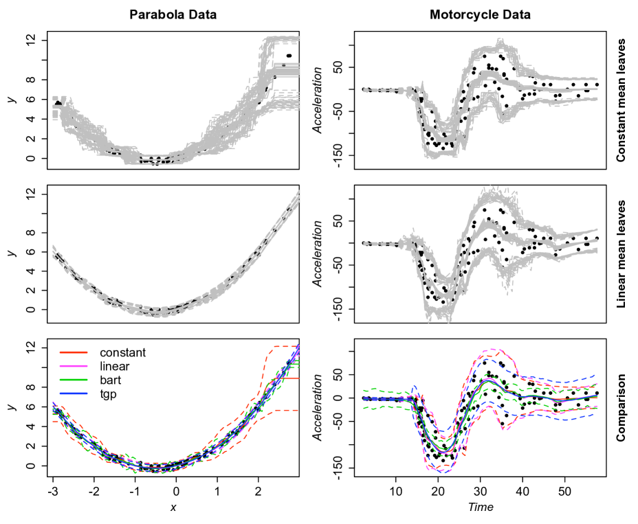
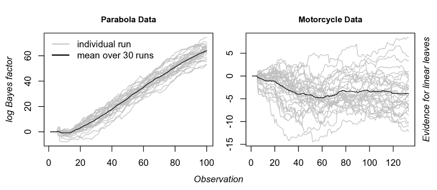
Figure 2: Top two rows show, for constant and linear leaves, posterior mean and 90% interval for each of 30 runs with 1000 particles to randomly ordered data. Bottom row shows mean and 90% interval for the average across dynamic tree runs, as well as for BART and TGP.

Figure 3: Filtered log Bayes factors for linear against constant leaf tree models, calculated for 30 random data orderings (the mean is shown in black) with 1000 particles.

Finally, the bottom row of Figure 3 compares the means of the 30 dynamic tree fits to two similar modern nonparametric regression techniques: treed Gaussian processes (TGP) and Bayesian additive regression trees (BART; Chipman et al., , 2010). Each new model is designed as an extension to constant or linear regression trees, and makes steps to partially alleviate the mixing problems of CGM’s original MCMC inference. As mentioned previously, TGP takes advantage of a more flexible leaf regression model to allow for broader covariate partitions. In a different approach, BART proposes a mixture of relatively short trees, and the authors show that combinations of simple individual partitioning schemes can lead to a complicated predictive response surface. The TGP model is given 10 restarts of a 10,000 iteration MCMC run, while BART results are based on a single 1,100 iteration chain. For the parabola data, all of the models find practically identical fits, except for the poorly performing constant leaf dynamic tree. However, for the motorcycle data, we see that each model leads to mean functions that are very similar, but that posterior predictive 90% intervals for BART and TGP appear to variously over or under estimate data uncertainty around the regression mean. In particular, BART’s global variance term is misspecified for this heteroskedastic data.

To benchmark our methods on a more realistic high-dimensional example, we also consider out-of-sample prediction for a Friedman test function (originally designed to illustrate multivariate adaptive regression splines (MARS) in Friedman, , 1991). The response is $10\sin(\pi x_{1}x_{2})+20(x_{3}-0.5)^{2}+10x_{4}+5x_{5}$ with $\mathrm{N}(0,1)$ additive error. Our comparators, and their R implementations, are: treed constant (TC) and linear (TL) models, and GP models from tgp (Gramacy and Taddy, , 2009); MARS from mda (Leisch et al., , 2009); Random Forests (RF) from randomForest (Liaw and Wiener, , 2002); BART from BayesTree (Chipman and McCulloch, , 2009); and neural networks with 2-3 hidden layers from the nnet library.

For this experiment, 100 random training and prediction sets, of respective size 200 and 1000, were drawn with inputs uniform on $[0,1]^{5}$. Following Chipman et al., (2002), we measure performance through predictive root mean-square error (RMSE) to the true mean, and results are shown in Figure 4. Dynamic tree models (DTC/DTL) were fit in a single (random) pass with $N=1000$ particles, and the number of MCMC iterations and restarts, etc., for other Bayesian methods was such that Monte Carlo error in RMSE for repeated runs on the same data is negligible against the results in Figure 4. Non-Bayesian comparators were fit under package defaults. The dynamic versions of the tree models clearly outperform their static counterparts, and the dynamic treed linear model (DTL) performs nearly as well as or better than the GP and BART, both of which offer flexible mean functions under a (true) constant variance term.

	RMSE
method	mean	(sd)
GP	0.723	(0.053)
DTL	0.917	(0.104)
BART	0.935	(0.063)
TL	1.244	(0.217)
MARS	1.513	(0.072)
NNET2	1.913	(0.429)
NNET1	2.246	(0.424)
RF	2.320	(0.093)
DTC	2.459	(0.074)
TC	3.067	(0.102)

Figure 4: Predictive RMSE on the Friedman data; sample of 100 for each estimator.

fnum@subsection3.2 Search Optimization

In Taddy et al., (2009), TGP regression was used to augment a local pattern search scheme with ranked lists of locations that maximize a measure of expected improvement. The GP leaf model was successful in this setting – deterministic optimization with 8 inputs – but pairwise covariance calculations and repeated MCMC runs became unwieldy in higher dimensions. At the same time, such hybrid optimization schemes are most useful in complicated high-dimensional settings: although true global optimization is impossible without great expense, a hybrid method uses regression to locate promising input areas and move the local search appropriately, thus iterating towards robust optimality.

We propose that our dynamic regression trees, due to a flexible on-line inference framework, provide a very attractive regression tool for hybrid local-global search optimization. Although they are not interpolators, and thus of limited usefulness in deterministic optimization, both constant and linear regression trees provide an efficient model for the prediction and optimization of stochastic functions. Such stochastic optimization problems are common in operations research and, despite being deterministic, many engineering codes are more properly treated as stochastic due to numerical instability. This section will outline use of dynamic regression trees for the global component of a stochastic optimization search.

We seek to explore the input space in areas that are likely to provide the optimum response (by default, a minimum). In the deterministic setting, Jones et al., (1998) search for inputs which maximize the posterior expectation of an improvement statistic, $\mathrm{max}\{f_{min}-f(\mathbf{x}),0\}$. In more generality, improvement is just the utility derived from a new observation. For global search optimization, there is no negative consequence of an evaluation that does not yield a new optimum (this information is useful), and the utility of a point which does provide a new optimum is, say, linear in the difference between mean responses (other quantiles or moments are also possible). Thus, the improvement for a stochastic objective $y(\mathbf{x})$ after $t$ observations is $I(\mathbf{x})=\mathrm{max}\left\{\hat{y}_{\mathrm{min}}-\hat{y}(\mathbf{x}),0\right\},$ where $\hat{y}(\mathbf{x})$ is the regression model mean function (e.g., $\hat{y}(\mathbf{x})=\mu_{\eta}$ for constant leaves or $\hat{y}(\mathbf{x})=\mu_{\eta}+\mathbf{x}^{\prime}\beta_{\eta}$ for linear leaves) and $\hat{y}_{\mathrm{min}}$ is this expected response minimized over the input domain.

In hybrid schemes, we have found that maximizing $\mathds{E}[I(\mathbf{x})]$ can be overly myopic. We thus incorporate an active learning idea (refer to Section 3.3), and instead search for the maximizing argument to $G(\mathbf{x};\phi)=\mathds{E}[I(\mathbf{x})]+\mathrm{sd}(\hat{y}(\mathbf{x}))/\phi$, where $\phi$ is a precision parameter that can be decreased to favor a more global scope. Conveniently, use of constant or linear leaves allows for both $\mathds{E}[I(\mathbf{x})]$ and $\mathrm{sd}(\hat{y}(\mathbf{x}))$ to be calculated in closed form conditional on a given tree. In particular, with $\mathrm{St}(a_{\eta}(\mathbf{x}),b_{\eta}(\mathbf{x}),c_{\eta})$ the posterior for $\hat{y}(\mathbf{x})$ given tree $\mathcal{T}_{t}$ and $\hat{y}_{\mathrm{min}}$ fixed at the minimum for $a_{\eta}(\cdot)$ over our input domain, expected improvement $\mathds{E}[I]$ is (suppressing $\mathbf{x}$)

$$(\hat{y}_{\mathrm{min}}-a_{\eta})\mathrm{T}_{c_{\eta}}\left(\frac{\hat{y}_{\mathrm{min}}-a_{\eta}}{\sqrt{b_{\eta}}}\right)+\frac{\sqrt{b_{\eta}}}{c_{\eta}-1}\left[c_{\eta}+\frac{(\hat{y}_{\mathrm{min}}-a_{\eta})^{2}}{b_{\eta}}\right]\mathrm{t}_{c_{\eta}}\left(\frac{\hat{y}_{\mathrm{min}}-a_{\eta}}{\sqrt{b_{\eta}}}\right),$$

with $\mathrm{T}_{c}$ and $\mathrm{t}_{c}$ the standard $t$ cumulative distribution and density, respectively, with $c$ degrees of freedom (this is similar to the marginal improvement derived in Williams et al., , 2000). Finally, since $\mathds{E}[I]=\frac{1}{N}\sum_{i=1}^{N}\mathds{E}[I\mid\mathcal{T}^{(i)}]$ and $\mathrm{\mathds{V}ar}(\hat{y})=\mathds{E}[\mathrm{\mathds{V}ar}(\hat{y}\mid\mathcal{T})]+\mathrm{\mathds{V}ar}(\mathds{E}[\hat{y}\mid\mathcal{T}])$, it is possible to obtain $G=\mathds{E}[I]+\mathrm{sd}(\hat{y})/\phi$ by evaluating the appropriate functionals conditional on each $\mathcal{T}\in\{\mathcal{T}_{t}^{(i)}\}_{i=1}^{N}$ before taking moments across particles (see Section 3.3 for further detail).

In a generic approach to sequential design, which is also adopted in the active learning algorithms of Section 3.3, the choice of the “next point” for evaluation is based on criteria optimization over a discrete set of candidate locations. After initializing with a small number of function evaluations, each optimization step augments the existing sample $[\mathbf{x},y]^{t}$ by drawing a space-filling design (we use uniform Latin hypercube samples) of candidate locations, $\tilde{\mathbf{X}}=\{\tilde{\mathbf{x}}_{i}\}_{i=1}^{M}$, and finding $\mathbf{x}^{\star}\in\tilde{\mathbf{X}}$ which maximizes $G(\mathbf{x}^{\star})$. Next, evaluate the new location, set $[\mathbf{x}_{t+1},y_{t+1}]=[\mathbf{x}^{\star},y(\mathbf{x}^{\star})]$, and follow the steps in Section 2.3 to obtain an updated particle approximation to the tree posterior. This is repeated as necessary.

Figure 5 shows some results for mean optimization of the test function $y=\mathrm{sin}(x)-\mathrm{Cauchy}(x;1.6,0.15)+\varepsilon$, with $\varepsilon\sim\mathrm{N}(0,\sigma=0.1)$, for precision values $\phi=1$ and $\phi=10$. The fitted regression trees assume linear leaves and, in each case, we used 500 particles and 100 candidate locations. The role of $\phi$ in governing global scope is clear, as the higher precision search is quickly able to locate a robust minimum but does not then proceed with wider exploration. The linear leaf model seems to be efficient at fitting our test function.

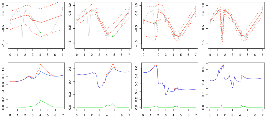
Iterations 10, 20, 40, and 60 with $\phi=1$.

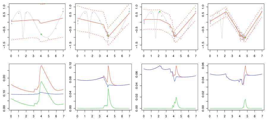
Iterations 2, 15, 30, and 45 with $\phi=10$.

Figure 5: Optimization with dynamic regression trees. For each iteration, posterior mean and 90% interval are on top (with true function and data in grey, and “next point” in green), while the bottom plot has $\mathds{E}[I]$ in green, $\mathrm{sd}(\hat{y})$ in blue, and $G=\mathds{E}[I]+\mathrm{sd}(\hat{y})/\phi$ in red.

Constant tree                         Linear tree                         Treed GP $\phi=100$ $\phi=10$ $\phi=1$ $\phi=100$ $\phi=10$ $\phi=1$ $g=1$ $g=5$ $g=10$ $-0.20$ $-0.21$ $-0.17$ $-0.04$ $-0.07$ $-0.05$ $-0.10$ $-0.08$ $-0.13$ $(0.13)$ $(0.15)$ $(0.15)$ $(0.09)$ $(0.13)$ $(0.09)$ $(0.12)$ $(0.10)$ $(0.14)$

Table 1: Minimization of the 2-d exponential function. For each optimization scheme, the top number is mean solution and the bottom number is standard deviation (out of 50 runs).

We also consider mean optimization of the two dimensional exponential function $y\sim\mathrm{N}(x_{1}\exp(-x_{1}^{2}-x_{2}^{2}),10^{-6})$, which is discussed further in Section 3.3. Given data from a random initial sample of 10 locations, our search routine was used to obtain the next 10 function evaluations, with $\phi=1$, $10$, or $100$, using 1000 particles and candidate sets of 200 locations. A TGP-based search optimization, as described in Gramacy and Taddy, (2010a), was also applied. This routine is the same as that outlined above for dynamic trees, except that it maximizes $\mathds{E}[I^{g}]$ rather than $G$, where each iteration requires a new MCMC run (we use 500 iterations after a burn-in of 500), and the candidate set is augmented with the location minimizing predicted response (such adaptation will often lead to a more efficient search). In this, the $g$ parameter increases the global scope (refer to Schonlau et al., , 1998) and we consider $g=1$, $5$, or $10$. Each optimization scheme was repeated 50 times, and the summary is shown in Table 1.

In a result that will parallel findings in Section 3.3, constant, rather than linear, leaves lead to a better exploration of the 2-d exponential function; this relative weakness exposes a difficulty for linear models in fitting the rapid oscillations around $(0,0)$. Interestingly, constant trees also lead to better results than for the TGP optimization routine. This is despite the added flexibility of GP leaves, an augmented candidate sample, and use of a wide range of $g$ values for $\mathds{E}[I^{g}]$ (which, although harder to compute when marginalizing over model parameters, is the literature standard for this type of search). In addition, due to repeated MCMC runs, the TGP algorithm requires near to 10 times the computation of sequential tree optimization.

fnum@subsection3.3 Active Learning

Another common application of sequential design is focused on evaluating an unknown response surface – the mean function $f(\mathbf{x})$ in (1.a) – at its most informative input location. Such active learning procedures are intended to provide efficient automatic exploration of the covariate space, thus guiding an on-line minimization of prediction error. As in the search optimization of Section 3.2, each active learning iteration will draw candidate locations, $\tilde{\mathbf{X}}=\{\tilde{\mathbf{x}}_{i}\}_{i=1}^{M}$, and select the next ($t+1^{\mathrm{st}}$) design point to be $\mathbf{x}^{\star}\in\tilde{\mathbf{X}}$ which maximizes a heuristic statistic. However, instead of aiming for a function optimum, we are now solely interested in understanding the response surface over some specified input range. Hence, we need to choose $\mathbf{x}^{\star}$ to maximize some measure of the predictive information gained by sampling $y(\mathbf{x^{\star}})$.

Two common heuristics for this purpose are active learning MacKay, (ALM; 1992) and active learning Cohn, (ALC; 1996). An ALM scheme selects the $\mathbf{x}^{\star}$ that leads to maximum variance for $y(\mathbf{x}^{\star})$, whereas ALC chooses $\mathbf{x}^{\star}$ to maximize the expected reduction in predictive variance averaged over the input space. A comparison between approaches depends upon the regression model and the application, however it may be shown that both approximate a maximum expected information design and that ALC improves upon ALM under heteroskedastic noise. Both heuristics have computational demands that grow with $|\tilde{\mathbf{X}}|$: ALC requires time in $O(|\tilde{\mathbf{X}}|^{2})$, wheres ALM is in $O(|\tilde{\mathbf{X}}|)$. Gramacy and Lee, (2009) provide further discussion of active learning as well as extensive results for ALC and ALM schemes based on MCMC inference with CGM’s static treed constant/linear (TC/L) models, GPs, and TGPs.

Since active learning is an inherently on-line algorithm, it provides a natural application for dynamic regression trees. The remainder of this section will illustrate ALC/ALM schemes built around particle learning for trees, and show that our methods compare favorably to existing MCMC-based alternatives. As in 3.2, both constant and linear leaf models lead to closed-form calculations of heuristic functionals conditional on a given tree. Fast prediction allows us to evaluate the necessary statistics across candidates, for each particle, and hence find the optimal $\mathbf{x}^{\star}$ under our heuristic. Trees are then updated for $y(\mathbf{x}^{\star})$, and the process is repeated.

ALM seeks to maximize $\mathrm{\mathds{V}ar}(y(\mathbf{x}))$, which is fairly simple to calculate. For a given tree $\mathcal{T}_{t}$ such that $\mathbf{x}$ is allocated to leaf node $\eta\in L_{\mathcal{T}_{t}}$, let $\mu_{\eta}(\mathbf{x})=\mathds{E}[y(\mathbf{x})\mid\eta]$ and $\mathrm{v}_{\eta}(\mathbf{x})=\mathrm{\mathds{V}ar}(y(\mathbf{x})\mid\eta)$ denote the conditional predictive mean and variance respectively for $y(\mathbf{x})$. These are available from equations (7) and (10) for each leaf model as $\mu_{\eta}(\mathbf{x})=\bar{y}_{\eta}$ or $\mu_{\eta}(\mathbf{x})=\bar{y}_{\eta}+\hat{\mathbf{x}}^{\prime}\hat{\beta}_{\eta}$ and $\mathrm{v}_{\eta}(\mathbf{x})=s_{\eta}^{2}(1+{1}/{|\eta|})/(|\eta|-3)$ or $\mathrm{v}_{\eta}(\mathbf{x})=[s_{\eta}^{2}-\mathcal{R}_{\eta}]\left(1+{1}/{|\eta|}+\hat{\mathbf{x}}^{\prime}\mathcal{G}_{\eta}^{-1}\hat{\mathbf{x}}\right)/(|\eta|-d-3)$. Given the particle set $\{\mathcal{T}_{t}^{(i)}\}_{i=1}^{N}$, the unconditional predictive variance is

$$\mathrm{\mathds{V}ar}(y(\mathbf{x})) =\mathds{E}[\mathrm{\mathds{V}ar}(y(\mathbf{x})\mid\mathcal{T})]+\mathrm{\mathds{V}ar}(\mathds{E}[y(\mathbf{x})\mid\mathcal{T}])$$

$$\approx\frac{1}{N}\left[\sum_{i=2}^{N}\mathrm{v}^{(i)}_{\eta}(\mathbf{x})+\mu^{(i)}_{\eta}(\mathbf{x})^{2}\right]-\left[\frac{1}{N}\sum_{i=1}^{N}\mu^{(i)}_{\eta}(\mathbf{x})\right]^{2},$$ (16)

which is straightforward to evaluate for all $\mathbf{x}\in\tilde{\mathbf{X}}$ during our search for the maximizing $\mathbf{x}^{\star}$.

The ALC statistic is more complicated. Let $\Delta\sigma^{2}_{\mathbf{x}}(\mathbf{x}^{\prime})=\mathrm{\mathds{V}ar}(y(\mathbf{x}^{\prime}))-\mathrm{\mathds{V}ar}(y(\mathbf{x}^{\prime})\mid\mathbf{x}^{\prime})$ denote the reduction in variance at $\mathbf{x}^{\prime}$ when the design is augmented with $\mathbf{x}$. Since $y(\mathbf{x})$ is not observed, the ALC statistics must condition on the existing model state. Hence, we define $\Delta\sigma^{2}_{\mathbf{x}}(\mathbf{x}^{\prime})=\mathds{E}[\Delta\sigma^{2}_{\mathbf{x}}(\mathbf{x}^{\prime}\mid\mathcal{T}_{t})]$ at time $t$ in terms of the conditional variance reduction

$$\Delta\sigma^{2}_{\mathbf{x}}(\mathbf{x}^{\prime}\mid\mathcal{T}_{t})=\mathrm{\mathds{V}ar}(y(\mathbf{x}^{\prime})\mid\mathcal{T}_{t})-\mathrm{\mathds{V}ar}(y(\mathbf{x}^{\prime})\mid\mathbf{x},\mathcal{T}_{t}).$$ (17)

Expressions for $\Delta\sigma^{2}_{\mathbf{x}}(\mathbf{x}^{\prime}\mid\mathcal{T}_{t})$ may be obtained as a special case of the results given by Gramacy and Lee, (2009). Clearly, $\Delta\sigma^{2}_{\mathbf{x}}(\mathbf{x}^{\prime}\mid\mathcal{T}_{t})=0$ if $\mathbf{x}$ and $\mathbf{x}^{\prime}$ are allocated to different leaves of $\mathcal{T}_{t}$. Otherwise, for $\mathbf{x}$ and $\mathbf{x}^{\prime}$ allocated to $\eta\in L_{\mathcal{T}_{t}}$ in a given tree, we have that $\Delta\sigma^{2}_{\mathbf{x}}(\mathbf{x}^{\prime}\mid\mathcal{T}_{t})=\Delta\sigma^{2}_{\mathbf{x}}(\mathbf{x}^{\prime}\mid\eta)$ is (for constant and linear leaves respectively)

$$\frac{s_{\eta}^{2}}{|\eta|-3}\times\frac{\left(\frac{1}{|\eta|}\right)^{2}}{1+\frac{1}{|\eta|}}~{}~{}~{}~{}~{}\mbox{or}~{}~{}~{}~{}~{}\frac{s_{\eta}^{2}-\mathcal{R}_{\eta}}{|\eta|-m-3}\times\frac{\left(\frac{1}{|\eta|}+(\hat{\mathbf{x}}^{\prime})^{\prime}\mathcal{G}^{-1}_{\eta}\hat{\mathbf{x}}\right)^{2}}{1+\frac{1}{|\eta|}+(\hat{\mathbf{x}}^{\prime})^{\prime}\mathcal{G}^{-1}_{\eta}\hat{\mathbf{x}}},$$ (18)

where $\hat{\mathbf{x}}=\mathbf{x}-\bar{\mathbf{x}}_{\eta}$ and similarly for $\hat{\mathbf{x}}^{\prime}$. In practice, the integral $\Delta\sigma^{2}(\mathbf{x})=\int_{\mathbb{R}^{d}}\Delta\sigma^{2}_{\mathbf{x}}(\mathbf{x}^{\prime})\,d\mathbf{x}^{\prime}$ is approximated by a discrete sum over the random space-filling set $\tilde{\mathbf{X}}$. Hence, $\mathbf{x}^{\star}$ is the candidate location which maximizes the sum of $\Delta\sigma^{2}_{\mathbf{x}^{\star}}(\mathbf{x}^{\prime}\mid\mathcal{T}_{t})$ over both $\mathbf{x}^{\prime}\in\tilde{\mathbf{X}}$ and $\mathcal{T}_{t}\in\{\mathcal{T}_{t}^{(i)}\}_{i=1}^{N}$.

We use the parabola and motorcycle data examples of Section 3.1 to compare ALC and ALM for both constant and linear leaf dynamic trees. Figure 6 illustrates the statistics associated with each combination of the two heuristics and two regression models, evaluated given the complete datasets. For the parabola data (left column), the ALM and ALC plots look roughly similar and, in each case, the linear model statistics are much more flat than for the constant model. In contrast, the ALM and ALC plots are very different from each other for the motorcycle data, which exhibit heteroskedastic additive error.

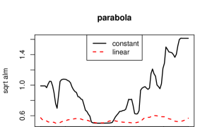
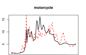
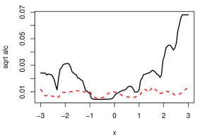
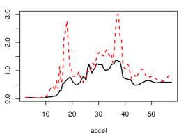
Figure 6: Active learning comparison for the parabola (left) and motorcycle data (right). The top row shows $\mathrm{\mathds{V}ar}(y(\mathbf{x}))$ for ALM and the bottom shows $\sqrt{\Delta\sigma^{2}(\mathbf{x})}$ for ALC.

$t=10$	$t=25$	$t=55$

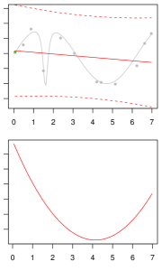
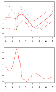
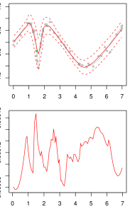
Figure 7: Snapshots showing the progression of the ALC heuristic driven by the dynamic tree model with linear leaves on the sin/Cauchy test data. The top panels show the true surface (grey lines), sampled input/output pairs (grey points), and the dynamic tree predictive means and 90% quantiles (red lines). The bottom panels show the corresponding $\Delta\sigma^{2}(\mathbf{x})$ surface.

1-d Sin/Cauchy
model	design	RMSE
TGP	ALC	0.0641
TGP	ALM	0.0660
DTL	ALC	0.0755
GP	ALM	0.0847
DTL	ALM	0.0992
–	LHS	0.1251
GP	ALC	0.1265
–	ME	0.1325
TC	ALC	0.1597
DTC	ALC	0.1616
TC	ALM	0.1960
TL	ALC	0.2193
DTC	ALM	0.2251
TL	ALM	0.2458

2-d Exponential
model	design	RMSE
TGP	ALM	0.00577
DTC	ALC	0.00732
DTL	ALM	0.00740
TGP	ALC	0.00852
DTL	ALC	0.00936
DTC	ALM	0.00997
TC	ALM	0.01126
TC	ALC	0.01182
TL	ALM	0.01622
GP	ALM	0.02411
TL	ALC	0.02431
–	LHS	0.03636
–	ME	0.04408
GP	ALC	0.05419

Table 2: Comparing models and active learning heuristics on the 1-d sin/Cauchy data and the 2-d exponential data. The tables are sorted on the fourth column (RMSE).

For a further comparison we return to the sin/Cauchy data from Section 3.2. Figure 7 shows sequential design progress under our dynamic tree model with linear leaves and the ALC heuristic in three snapshots: after an initial $t=10$ Latin hypercube (LHS) sample, after 15 samples taken via ALC ($t=25$) and after 45 ALC samples ($t=55$). With the exception of $t=10$, when there is not enough data to support a split in the tree(s), the ALC statistic is high at points where $y(\mathbf{x})$ is changing direction—highest where it is changing most rapidly.

Table 2 (left) shows how the dynamic tree models compare to various static Bayesian treed models, including TGP, on this data. All experiments were started with an initial LHS in $[0,7]$ of size 10 followed by 40 active learning rounds. Each round uses 20 random LHS candidates $\tilde{\mathbf{X}}$ in $[0,7]$. At the end of the 40 rounds the root mean squared error (RMSE) was calculated for a comparison of predictive means to the truth in a size 200 hold-out set from a GP-based maximum entropy (ME) design in $[0,7]$. This was repeated 30 times and the average RMSE is shown in the table. The expensive TGP methods dominate, with dynamic trees using linear leaves (DTL) trailing. In both cases, ALC edges out ALM. Interestingly, while static treed linear models (TL) fit through MCMC are amongst the worse performers, their sequential alternatives are amongst the best. Neither TC or DTC are strong performers, perhaps due to the almost linear derivatives of our test function. Since the “interesting” aspects of this response are evenly distributed throughout the input space, both the GP with ALM and the offline LHS and ME comparators also do well.

Table 2 (right) shows the results of a similar experiment for the 2-d exponential data from Section 3.2. The setup is as described above, except that the initial LHS is now of size 20 and is followed by 55 active learning rounds. Here, the dynamic trees share the top 6 spots with TGP only, and clearly dominate their static analogues. Indeed, DTC is the second best performer, echoing our findings in Section 3.2 that the constant leaf model is a good fit for this function. In contrast to the results from our simple 1-d example, the offline (LHS and ME) and GP methods are poor here because the region of interest is confined to the bottom left quadrant of our 2-d input space. Finally, in all of these examples, dynamic regression trees (DTC and DTL) are the only methods that run on-line and do not require batch MCMC processing.

fnum@subsection3.4 Classification

Classification is one of the original applications for tree models, and is very often associated with sequential inference settings. Categorical data can be fit with multinomial leaf trees (as in 2.2.3) and, without an application specific loss function, the predictive classification rule assigns to new inputs the class with highest mean conditional posterior probability. That is,

$$\hat{c}(\mathbf{x})=\mathrm{arg~{}max}\left\{\frac{1}{N}\sum_{i=1}^{N}\left(\hat{p}^{\eta(\mathbf{x})}_{c}\right)^{(i)}:~{}{c=1,\ldots,C}\right\},$$ (19)

for a set of $N$ particles, where each $\hat{p}^{\eta(\mathbf{x})}_{c}$ is the $c$-class probability from (13) for the leaf corresponding to $\mathbf{x}$. Evaluating $\hat{c}(\mathbf{x})$ over the input space provides a predictive classification surface.

We first apply our methodology to the Cushing’s data, again available in the MASS library for R, used throughout the book by Ripley, (1996) to illustrate various classification algorithms. This simple data set has two inputs – each patient’s urinary excretion rates for tetrahydrocortisone and pregnanetriol, considered on the log scale – and the response is one of three different types of Cushing’s syndrome (referred to as $a$, $b$, or $c$). We fit the multinomial leaf dynamic tree model to this data, and compare our results to those from a GP soft-max classifier as outlined in Broderick and Gramacy, (2009), which fits independent GP models to each latent response $y_{c}$ such that $p_{c}=\mathrm{exp}({y_{c}})/\sum_{l=1}^{C}\mathrm{exp}({y_{l}})$.

Figure 8 illustrates the outcome of this example. The dynamic tree results (top row) are based on a set of 1000 particles, while the GP soft-max results (bottom row) use every 100^th observation of a 10,000 iteration MCMC chain. The left column of this figure shows the syndrome classification surface based on maximum mean posterior probability, as in (19). Although it is not possible to assess whether any classifier is outperforming the other, these surfaces clearly illustrate the effect of axis-symmetric (tree) classification as opposed to the surface from a radial-basis (GP) model. We also note that the GP soft-max classification rule is very similar to results from Ripley, (1996, chap. 5.2) for a neural network fit with weight decay.

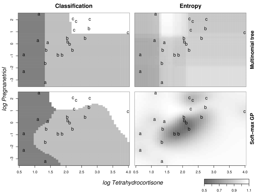
Figure 8: Cushing’s data example. The left column shows the class corresponding to maximum mean posterior probability, and the right has entropy for the posterior mean probability vector. Results for a dynamic classification tree are on top, and for a GP soft-max classifier on the bottom. Class (a$\rightarrow$c) and entropy rise from black to white, and plotted data is labelled by class.

The right column of Figure 8 shows the entropy, $-\sum_{l\in\{a,b,c\}}p_{l}\log(p_{l})$, of the posterior mean probability surface for each classification model. Such entropy plots, which are commonly used in classification settings to assess response variability, illustrate change in expected value of information over the input space. Indeed, Gramacy and Polson, (2010) propose entropy as an active learning criteria for classification problems, analogous to ALC in Section 3.3. In our application, dynamic tree entropy is peaked around a 3-class border region in the top-left. This intuitively offers better guidance about the value of additional information than the GP entropy surface, which is high everywhere except right at clusters of same-class observations.

To better assess the performance of our dynamic tree classifier, we turn to a larger “credit approval” data set from the UC Irvine Machine Learning Database. This data includes 690 credit card applicants grouped by approval status (either ‘+’ or ‘-’) and 15 input variables. Eleven of these inputs are categorical, and for each of these we have encoded the categories through a series of binary variables. This convenient reparametrization, which expands the input space to 47 dimensions, allows direct application of the model in Section 1.1 with nodes splitting on $x_{i}=0$ or $1$ for each binary variable (see Gramacy and Taddy, , 2010a, for discussion of this approach in general partition trees). As an aside, we note that the binary encoding can also be used to incorporate categorical data into constant and linear leaf trees; the only adaptation is, for linear leaves, to exclude binary variables from each regression design matrix.

We applied the multinomial dynamic tree to 100 independent repetitions of training on 90% of the credit approval data and predictive classification on the left-out 10% sample. This experiment is identical to that in Broderick and Gramacy, (2009), who tested both a TGP soft-max classifier (includes binary variables for partitioning of latent TGP processes and fits independent GP to continuous inputs within each partition) and a naïve GP soft-max classifier (fit to the reparametrized 47 inputs, treating binary variables as continuous in the correlation function). Their results are repeated here, beside those for our dynamic tree, in Table 3. Once again, despite using a less sophisticated leaf model, the dynamic tree is a clear performance winner and the only classifier able to beat 14% average missclassification. The dynamic tree was also orders-of-magnitude faster than the GP and TGP classifiers (we use 1000 particles, and they have 15,000 iterations), and only our approach will be feasible in on-line applications.

Classifier	Dynamic Multinomial Tree	TGP soft-max	GP soft-max
Missclassification rate	0.136 (0.038)	0.142 (0.036)	0.146 (0.04)
Time (CPU hours) per fold	0.01	1.62	5.52

Table 3: Mean (and standard deviation) for out-of-sample missclassification over 10 random 10-fold cross-validations and computing time for each classifier on the credit approval data.

4 Discussion

We have reformulated regression trees as a dynamic model. This sequential characterization leads to an entirely new class of models which can be fit on-line; have a scale-free automatic prior specification; avoid the need for parameter sampling; and lead to robust and flexible prediction. We have shown empirically that our dynamic regression trees can provide superior performance and are less expensive than common alternatives.

In a key point, we have been able to define particles for filtering which contain only split rules and sufficient statistics, leading our sequential filtering to efficiently discard all partition models except those which are predicting well. Due to the size and complexity of potential tree space, this narrowing of posterior search is an essential aspect of our models’ success. In addition, restrictions on partition size allow us to make use of improper priors (for constant and linear leaves), which is not usually possible in particle inference.

The modeling and examples contained herein provide encouragement for further work under a strategy that looks to take advantage of sequential model characterizations. In particular, we hope to find that similar ideas on update mechanisms for covariate dependent model features will lead to insight about dynamic versions of other graphical structures.

References

- Atkinson, (1978) Atkinson, A. C. (1978). “Posterior Probabilities for Choosing a Regression Model.” Biometrika, 65, 39–48.
- Breiman et al., (1984) Breiman, L., Friedman, J. H., Olshen, R., and Stone, C. (1984). Classification and Regression Trees. Belmont, CA: Wadsworth.
- Broderick and Gramacy, (2009) Broderick, T. and Gramacy, R. B. (2009). “Classification and Categorical Inputs with Treed Gaussian Process Models.” Tech. rep., University of Cambridge. arXiv:0904.4891.
- Cappé et al., (2005) Cappé, O., Douc, R., and Moulines, E. (2005). “Comparison of Resampling Schemes for Particle Filtering.” In 4th International Symposium on Image and Signal Processing and Analysis (ISPA). Zagreb, Croatia.
- Carvalho et al., (2010a) Carvalho, C. M., Johannes, M., Lopes, H. F., and Polson, N. G. (2010a). “Particle Learning and Smoothing.” Statistical Science, 25, 88–106.
- Carvalho et al., (2010b) Carvalho, C. M., Lopes, H. F., Polson, N., and Taddy, M. A. (2010b). “Particle Learning for General Mixtures.” Bayesian Analysis. To appear.
- Chipman and McCulloch, (2009) Chipman, H. and McCulloch, R. (2009). BayesTree: an R package implementing Bayesian Methods for Tree Based Models. R package version 0.3-1.
- Chipman et al., (1998) Chipman, H. A., George, E. I., and McCulloch, R. E. (1998). “Bayesian CART Model Search (with discussion).” Journal of the American Statistical Association, 93, 935–960.
- Chipman et al., (2002) — (2002). “Bayesian Treed Models.” Machine Learning, 48, 303–324.
- Chipman et al., (2010) — (2010). “BART: Bayesian Additive Regression Trees.” The Annals of Applied Statistics, 4, 266–298.
- Cohn, (1996) Cohn, D. A. (1996). “Neural Network Exploration using Optimal Experimental Design.” In Advances in Neural Information Processing Systems, vol. 6(9), 679–686. Morgan Kaufmann Publishers.
- Friedman, (1991) Friedman, J. H. (1991). “Multivariate Adaptive Regression Splines.” Annals of Statistics, 19, No. 1, 1–67.
- Gramacy and Lee, (2008) Gramacy, R. B. and Lee, H. K. H. (2008). “Bayesian Treed Gaussian Process Models with an Application to Computer Modeling.” Journal of the American Statistical Association, 103, 1119–1130.
- Gramacy and Lee, (2009) — (2009). “Adaptive Design and Analysis of Supercomputer Experiment.” Technometrics, 51, 2, 130–145.
- Gramacy and Polson, (2010) Gramacy, R. B. and Polson, N. G. (2010). “Particle Learning of Gaussian Process Models for Sequential Design and Optimization.” Journal of Computational and Graphical Statistics. To appear.
- Gramacy and Taddy, (2009) Gramacy, R. B. and Taddy, M. A. (2009). tgp: an R package for Bayesian treed Gaussian process models. R package version 2.3.
- Gramacy and Taddy, (2010a) — (2010a). “Categorical inputs, sensitivity analysis, optimization and importance tempering with tgp version 2.” Journal of Statistical Software, 33.
- Gramacy and Taddy, (2010b) — (2010b). dynaTree: an R package implementing dynamic trees for learning and design. R package version 1.0.
- Higdon et al., (1999) Higdon, D., Swall, J., and Kern, J. (1999). “Non-Stationary Spatial Modeling.” In Bayesian Statistics 6, eds. J. M. Bernardo, J. O. Berger, A. P. Dawid, and A. F. M. Smith, 761–768. Oxford University Press.
- Jones et al., (1998) Jones, D., Schonlau, M., and Welch, W. (1998). “Efficient Global Optimization of Expensive Black-Box Functions.” Journal of Global Optimization, 13, 455–492.
- Kass and Raftery, (1995) Kass, R. E. and Raftery, A. E. (1995). “Bayes factors.” Journal of the American Statistical Association, 90, 773–795.
- Kong et al., (1994) Kong, A., Liu, J. S., and Wong, W. H. (1994). “Sequential Imputations and Bayesian Missing Data Problems.” Journal of the American Statistical Association, 89, 278–288.
- Leisch et al., (2009) Leisch, F., Hornik, K., and Ripley, B. D. (2009). mda: an R package for Mixture and flexible discriminant analysis. R package version 0.4-1, S original by Trevor Hastie & Robert Tibshirani.
- Liaw and Wiener, (2002) Liaw, A. and Wiener, M. (2002). “Classification and Regression by randomForest.” R News, 2, 3, 18–22.
- MacKay, (1992) MacKay, D. J. C. (1992). “Information–based Objective Functions for Active Data Selection.” Neural Computation, 4, 4, 589–603.
- Pitt and Shephard, (1999) Pitt, M. K. and Shephard, N. (1999). “Filtering via Simulation: Auxiliary Particle Filters.” Journal of the American Statistical Association, 94, 590–599.
- Ripley, (1996) Ripley, B. D. (1996). Pattern Recognition and Neural Networks. Cambridge University Press.
- Santner et al., (2003) Santner, T. J., Williams, B. J., and Notz, W. I. (2003). The Design and Analysis of Computer Experiments. New York, NY: Springer-Verlag.
- Schonlau et al., (1998) Schonlau, M., Welch, W., and Jones, D. (1998). “Global versus local search in constrained optimization of computer models.” In New developments and applications in experimental design, 11–25. Institute of Mathematical Statistics.
- Taddy et al., (2009) Taddy, M. A., Lee, H. K. H., Gray, G. A., and Griffin, J. D. (2009). “Bayesian Guided Pattern Search for Robust Local Optimization.” Technometrics, 51, 389–401.
- Williams et al., (2000) Williams, B. J., Santner, T. J., and Notz, W. I. (2000). “Sequential Design of Computer Experiments to Minimize Integrated Response Functions.” Statistica Sinica, 10, 1133–1152.