Simulation of relativistic shocks and associated radiation

Abstract

Using our new 3-D relativistic electromagnetic particle (REMP) code parallelized with MPI, we investigated long-term particle acceleration associated with a relativistic electron-positron jet propagating in an unmagnetized ambient electron-positron plasma. We have also performed simulations with electron-ion jets. The simulations were performed using a much longer simulation system than our previous simulations in order to investigate the full nonlinear stage of the Weibel instability for electron-positron jets and its particle acceleration mechanism. Cold jet electrons are thermalized and ambient electrons are accelerated in the resulting shocks for both cases. Acceleration of ambient electrons leads to a maximum ambient electron density three times larger than the original value for pair plasmas. Behind the bow shock in the jet shock strong electromagnetic fields are generated. These fields may lead to time dependent afterglow emission. We calculated radiation from electrons propagating in a uniform parallel magnetic field to verify the technique. We also used the new technique to calculate emission from electrons based on simulations with a small system with two different cases for Lorentz factors (15 and 100). We obtained spectra which are consistent with those generated from electrons propagating in turbulent magnetic fields with red noise. This turbulent magnetic field is similar to the magnetic field generated at an early nonlinear stage of the Weibel instability.

I RPIC SIMULATIONS

Particle-in-cell (PIC) simulations can shed light on the physical mechanism of particle acceleration that occurs in the complicated dynamics within relativistic shocks. Recent PIC simulations of relativistic electron-ion and electron-positron jets injected into an ambient plasma show that acceleration occurs within the downstream jet  nishi03 ; silva03 ; fred04 ; nishi05 ; hede05 ; jaro05 ; nishi06 ; ram07 ; chang08 ; anat08a ; dsd08 ; anat08b ; sironi09m . In general, these simulations have confirmed that relativistic jets excite the Weibel instability, which generates current filaments and associated magnetic fields  weib59 ; medv99 , and accelerates electrons  hede05 ; nishi06 ; ram07 ; chang08 ; anat08a ; anat08b ; sironi09m .

Therefore, the investigation of radiation resulting from accelerated particles (mainly electrons and positrons) in turbulent magnetic fields is essential for understanding radiation mechanisms and their observable spectral properties. In this report we present a new numerical method to obtain spectra from particles self-consistently traced in our PIC simulations.

I.1 Relativistic Jets Injected into Unmagnetized Plasmas using a Large System

We have performed simulations using a system with ($L_{\rm x},L_{\rm y},L_{\rm z})=(4005\Delta,$ $131\Delta,131\Delta)$ ($\Delta=1$: grid size) and a total of $\sim 1$ billion particles (12 particles $/$cell$/$species for the ambient plasma) in the active grid zones  nishi09b . We have performed two kind of simulations: an electron-positron jet is injected into an ambient pari plasma and an electron-ion jet into electron-ion ambient plasma ($m_{\rm i}/m_{\rm e}=20$). In the simulations the electron skin depth, $\lambda_{\rm ce}=c/\omega_{\rm pe}=10.0\Delta$, where $\omega_{\rm pe}=(4\pi e^{2}n_{\rm e}/m_{\rm e})^{1/2}$ is the electron plasma frequency and the electron Debye length $\lambda_{\rm e}$ is half of the grid size. Here the computational domain is six times longer than in our previous simulations  nishi06 ; ram07 . The electron number density of the jet is $0.676n_{\rm e}$, where $n_{\rm e}$ is the ambient electron density and $\gamma=15$ for both cases. The electron/positron thermal velocity of the jet is $v^{\rm e}_{\rm j,th}=0.014c$, the ion thermal velocity where $c=1$ is the speed of light. The ion thermal velocity of jet is $v^{\rm i}_{\rm j,th}=v^{\rm e}_{\rm j,th}*\sqrt{m_{\rm e}/m_{\rm i}}=0.00313c$. The electron/positron thermal velocity in the ambient plasma is $v^{\rm e}_{\rm a,th}=0.05c$ ($v^{\rm i}_{\rm a,th}=0.0112c$).

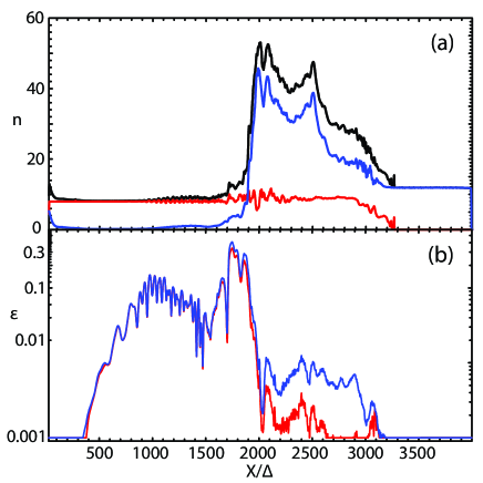
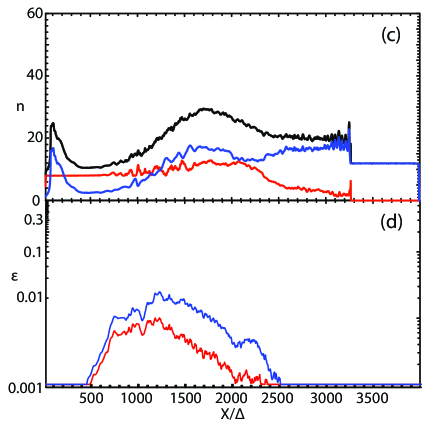
Figure 1: The averaged values of electron density (a, c) and field energy (b, d) along the $x$ at $t=3750\omega_{\rm pe}^{-1}$. The left panel (Figs. 1a and 1b) is for the case of pair plasmas and the right panel (Figs. 1c and 1d) is for the electron-ion case ($m_{\rm i}/m_{\rm e}=20$). Figs. 1a and 1c show jet electrons (red), ambient electrons (blue), and the total electron density (black). Figs. 1b and 1d show electric field energy (red) and magnetic field energy (blue) divided by the total kinetic energy.

Figure 1 shows the averaged (in the $y-z$ plane) electron density and electromagnetic field energy along the jet at $3750\omega_{\rm pe}^{-1}$ for electron-positron (Figs. 1a and 1b) and electron-ion (Figs. 1c and 1d) jets. The resulting profiles of jet (red), ambient (blue), and total (black) electron density are shown in Figs. 1a and 1c. The ambient electrons are accelerated by the jet electrons and pile up towards the front part of jet. For electron-positron jet, at the earlier time the ambient plasma density increases linearly behind the jet front. At the later time the ambient plasma shows a rapid increase to a plateau behind the jet front, with additional increase to a higher plateau farther behind the jet front. The jet density remains approximately constant except near the jet front.

The acceleration of ambient electrons becomes visible when jet electrons pass about $x/\Delta=500$. The maximum density of accelerated ambient electrons is attained at $t=1750\omega_{\rm pe}^{-1}$. The maximum density gradually reaches a plateau as seen in Fig. 1a. The maximum electromagnetic field energy is located at $x/\Delta=1,700$ as shown in Fig. 1b.

The Weibel instability remains excited by continuously injected jet particles and the electromagnetic fields are maintained at a high level, about four times that seen in a previous, much shorter grid simulation system ($L_{\rm x}=640\Delta$). At the earlier simulation time a large electromagnetic structure is generated and accelerates the ambient plasma. As shown in Fig. 1b, at the later simulation time the strong magnetic field extends up to $x/\Delta=2,000$. These strong fields become very small beyond $x/\Delta=2000$ in the shocked ambient region  nishi06 ; ram07 .

In the case with electron-ion jet, due to the heavier ions at $3750\omega_{\rm pe}^{-1}$ the density is piled up only slightly (Fig. 1c). The generated electromagnetic fields are smaller than those for the electron-positron case. Furthermore, in the front of electron-ion jet the electromagnetic fields disappear as shown in Fig. 1d. In order to generate a shock it will require at least several time longer simulations.

II THE STANDARD SYNCHROTRON RADIATION MODEL

A synchrotron shock model is widely adopted to describe the radiation mechanism in the external shock thought to be responsible for observed broad-band GRB afterglows  zm04 ; p05a ; Piran (2005b); zhangr07 ; nakar07 . Associated with this model are three major assumptions that are adopted in almost all current GRB afterglow models. Firstly, electrons are assumed to be “Fermi” accelerated at the relativistic shocks and to have a power-law distribution with a power-law index $p$ upon acceleration, i.e. $N(E_{\rm e})dE_{\rm e}\propto E^{-p}dE_{\rm e}$. This is consistent with recent PIC simulations of the shock formation and particle acceleration  anat08b and also some Monte Carlo models  Achterberg01 ; ellison02 ; lemoi03 , but see  niemiec06 ; niemiecp06 . Secondly, a fraction $\epsilon_{\rm e}$ (generally taken to be $\leq 1$) of the total electrons associated with ISM baryons are accelerated, and the total electron energy is a fraction $\epsilon_{\rm e}$ of the total internal energy in the shocked region. Thirdly, the strength of the magnetic fields in the shocked region is unknown, but its energy density ($B^{2}/8\pi$) is assumed to be a fraction $\epsilon_{B}$ of the internal energy. These assumed “micro-physics” parameters, $p,\epsilon_{\rm e}$ and $\epsilon_{\rm B}$, whose values are obtained from spectral fits  paku01 ; yost03 reflect a lack of knowledge of the underlying microphysics  wax06 .

The typical observed emission frequency from an electron with (comoving) energy $\gamma_{\rm e}m_{\rm e}c^{2}$ in a frame with a bulk Lorentz factor $\Gamma$ is $\nu=\Gamma\gamma_{\rm e}^{2}(eB/2\pi m_{\rm e}c)$. Three critical frequencies are defined by three characteristic electron energies. These are $\nu_{\rm m}$ (the injection frequency), $\nu_{\rm c}$ (the cooling frequency), and $\nu_{\rm M}$ (the maximum synchrotron frequency). In our simulations of GRB afterglows, there is one additional relevant frequency, $\nu_{\rm a}$, due to synchrotron self-absorption at lower frequencies  mrw98 ; spn98 ; zhangr07 ; nakar07 .

The general agreement between the blast wave dynamics and the direct measurements of the fireball size argue for the validity of this model’s dynamics  zhangr07 ; nakar07 . The shock is most likely collisionless, i.e. mediated by plasma instabilities  wax06 . The electromagnetic instabilities mediating the afterglow shock are expected to generate magnetic fields. Afterglow radiation was therefore predicted to result from synchrotron emission of shock accelerated electrons  mr97 . The observed spectrum of afterglow radiation is indeed remarkably consistent with synchrotron emission of electrons accelerated to a power-law distribution, providing support for the standard afterglow model based on synchrotron emission of shock accelerated electrons  p99 ; p00 ; p05a ; zm04 ; mes02 ; mes06 ; zhangr07 ; nakar07 .

In order to determine the luminosity and spectrum of synchrotron radiation, the strength of the magnetic field ($\epsilon_{\rm B}$) and the energy distribution of the electrons ($p$) must be determined. Due to the lack of a first principles theory of collisionless shocks, a purely phenomenological approach to the model of afterglow radiation was ascribed without investigating in detail the processes responsible for particle acceleration and magnetic field generation  wax06 . Rather, one simply assumes that a fraction $\epsilon_{\rm B}$ of the post-shock thermal energy density is carried by the magnetic field, that a fraction $\epsilon_{\rm e}$ is carried by electrons, and that the energy distribution of the electrons is a power-law, $d\log n_{\rm e}/d\log\varepsilon=p$ (above some minimum energy $\varepsilon_{0}$ which is determined by $\epsilon_{\rm e}$ and $p$), $\epsilon_{\rm B}$, $\epsilon_{\rm e}$ and $p$ are treated as free parameters, determined by observations. It is important to clarify here that the constraints implied on these parameters by the observations are independent of any assumptions regarding the nature of the afterglow shock and the processes responsible for particle acceleration or magnetic field generation. Any model should satisfy these observational constraints.

The properties of synchrotron (or “jitter”) emission from relativistic shocks will be determined by the magnetic field strength and structure and the electron energy distribution behind the shock. The characteristics of jitter radiation may be important to understanding the complex time evolution and/or spectral structure in gamma-ray bursts  pre98 . For example, jitter radiation has been proposed as a means to explain GRB spectra below the peak frequency that are harder than the “line of death” spectral index associated with synchrotron emission  medv00 ; medv06 , i.e., the observed spectral power scales as $F_{\nu}\propto\nu^{2/3}$, whereas synchrotron spectra are $F_{\nu}\propto\nu^{1/3}$ or softer  medv06 . Thus, it is essential to calculate radiation production by tracing electrons (positrons) in self-consistently treated small-scale electromagnetic fields.

III NEW NUMERICAL METHOD FOR CALCULATING SYNCHROTRON EMISSION

Let a particle be at position ${\bf{r}_{0}}(t)$ at time $t$  nishi09a ; hedeT05 ; hedeN05 . At the same time, we observe the electric field from the particle from position $\bf{r}$. However, because of the finite velocity of light, we observe the particle at an earlier position $\bf{r}_{0}(\rm{t}^{{}^{\prime}})$ where it was at the retarded time $t^{{}^{\prime}}=t-\delta t^{{}^{\prime}}=t-\bf{R}(\rm{t}^{{}^{\prime}})/c$. Here $\bf{R}(\rm{t}^{{}^{\prime}})=|\bf{r}-\bf{r}_{0}(\rm{t}^{{}^{\prime}})|$ is the distance from the charge (at the retarded time $t^{{}^{\prime}}$) to the observer.

After some calculation and simplifying assumptions the total energy $W$ radiated per unit solid angle per unit frequency from a charged particle moving with instantaneous velocity $\boldsymbol{\beta}$ under acceleration $\boldsymbol{\dot{\beta}}$ can be expressed as  rybi79 ; jack99

$$\frac{d^{2}W}{d\Omega d\omega} =$$

$$\frac{\mu_{0}cq^{2}}{16\pi^{3}} \left|\int^{\infty}_{\infty}\frac{\bf{n}\times[(\bf{n}-\mathbf{\beta})\times\dot{\bf{\beta}}]}{(1-\bf{\beta}\cdot\bf{n})^{2}}e^{i\omega(t^{{}^{\prime}}-\bf{n}\cdot\bf{r}_{0}(t^{{}^{\prime}})/c)}dt^{{}^{\prime}}\right|^{2}$$

Here, $\bf{n}\equiv\bf{R}(\rm{t}^{{}^{\prime}})/|\bf{R}(\rm{t}^{{}^{\prime}})|$ is a unit vector that points from the particle’s retarded position towards the observer.

The observer’s viewing angle is set by the choice of $\bf{n}$ ($n_{\rm x}^{2}+n_{\rm y}^{2}+n_{\rm z}^{2}=1$). The choice of unit vector $\bf{n}$ along the direction of propagation of the jet (hereafter taken to be the $x$-axis) corresponds to head-on emission. For any other choice of $\bf{n}$ (e.g., $\theta_{\gamma}=1/\gamma$), off-axis emission is seen by the observer.

III.1 Synchrotron radiation from two electrons propagating in parallel uniform magnetic field

In order to calculate radiation from relativistic jets propagating along the $x$ direction  nishi09a we consider a test case which includes a parallel magnetic field ($B_{\rm x}$), and jet velocity of $v_{\rm j1,2}=0.99c$. Two electrons are injected with different perpendicular velocities ($v_{\perp 1}=0.1c,v_{\perp 2}=0.12c$). A maximum Lorenz factor of $\gamma_{\max}=\{(1-(v_{\rm j2}^{2}+v_{\perp 2}^{2})/c^{2}\}^{-1/2}=13.48$ is calculated with the larger perpendicular velocity.

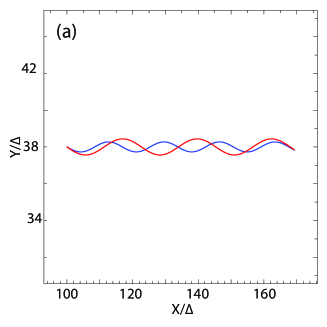
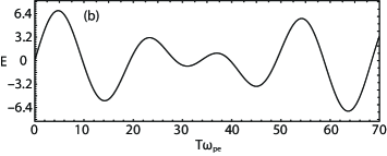
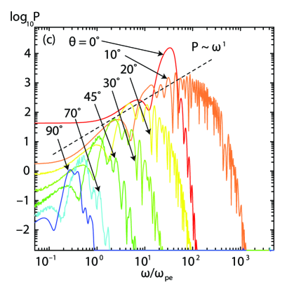
Figure 2: The case with a strong magnetic field ($B_{\rm x}=3.7$) and larger perpendicular velocity ($v_{\perp 1}=0.1c,v_{\perp 2}=0.12c$). The paths of two electrons moving helically along the $x-$direction in a homogenous magnetic field shown in the $x-y$-plane (a). The two electrons radiate a time dependent electric field. An observer situated at great distance along the n-vector sees the retarded electric field from the moving electrons at the rest frame (b). The observed power spectrum at different viewing angles from the two electrons (c). Frequency is in units of $\omega_{\rm pe}^{-1}$.

Figure 2 shows electron trajectories in the $x-y$ plane (red: $v_{\perp 2}=0.12c$, blue: $v_{\perp 1}=0.1c$) (a: left panel), the radiation (retarded) electric field (b: middle panel), and spectra (right panel) for the case $B_{\rm x}=3.70$. The two electrons are propagating left to right with gyration in the $y-z$ plane (not shown). The gyroradius is about $0.44\Delta$ for the electron with the larger perpendicular velocity. The seven curves show the power spectrum at viewing angles of 0^∘ (red), 10^∘ (orange), 20^∘ (yellow), 30^∘ (moss green), 45^∘ (green), 70^∘ (light blue), and 90^∘ (blue). The higher frequencies become stronger at the $10^{\circ}$ viewing angle. The critical angle for off-axis radiation $\theta_{\gamma}=180^{\circ}/(\pi\gamma_{\max})$ for this case is 4.25^∘. As shown in this panel, the spectrum at a larger viewing angle ($>20^{\circ}$) has smaller amplitude.

Since the jet plasma has a large velocity $x$-component in the simulation frame, the radiation from the particles (electrons and positrons) is strongly beamed along the $x$-axis (jitter radiation)  medv00 ; medv06 .

Equations 6.30a and 6.30b show that the radiation with the viewing angle $\alpha=0$ disappears (see Fig. 6.5 in the textbook of Rybicki and Lightman  rybi79 ). However, based on other textbooks, radiation at the viewing angle $0^{\circ}$ should not vanish  jack99 ; beke66 ; land80 . This aspect is shown in Fig. 2c, and at the higher frequency the amplitude at the viewing angle $10^{\circ}$ is stronger than that with viewing angle $0^{\circ}$.

III.2 Calculating Synchrotron and Jitter Emission from Electron Trajectories in Self-consistently Generated Magnetic Field

In order to validate our numerical method we performed simulations using a small system with ($L_{\rm x},L_{\rm y},L_{\rm z})=(645\Delta,131\Delta,131\Delta)$ ($\Delta=1$: grid size) and a total of $\sim 0.5$ billion particles (12 particles$/$cell$/$species for the ambient plasma) in the active grid zones  nishi06 . First we performed simulations without calculating radiation up to $t=450\omega_{\rm pe}^{-1}$. The jet front is located around about $x/\Delta=480$. We selected 12,150 electrons for each jet and ambient electrons randomly. Recently, a similar calculation has been carried out for the radiation from accelerated electrons in laser-wakefield acceleration  martins09 and in shocks  sironi09j .

Figure 3 shows (a) the current filaments generated by the Weibel instability and (b) the phase space of $x/\Delta-\gamma V_{\rm x}$ for jet electrons (red) and ambient electrons (blue) at $t=450\omega_{\rm pe}^{-1}$ for $\gamma=15$.

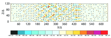
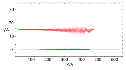
Figure 3: Two-dimensional images in the $x-z$ plane at $y/\Delta=65$ for $t=450\omega_{\rm pe}^{-1}$ for the case with $\gamma=15$. The colors indicate the x-component of current density generated by the Weibel instability, with the x- and z-components of magnetic field represented by arrows (a). Phase space distributions as a function of $x/\Delta-\gamma v_{\rm x}$ plotted for the jet (red) and ambient (blue) electrons at the same time.

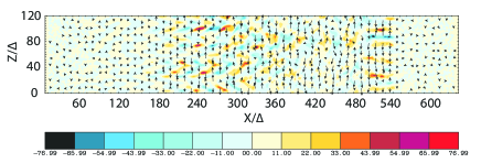
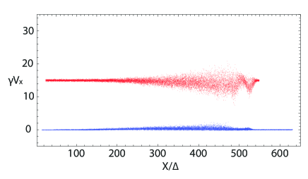
Figure 4: Two-dimensional images in the $x-z$ plane at $y/\Delta=65$ for $t=525\omega_{\rm pe}^{-1}$ for the case with $\gamma=15$. The colors indicate the x-component of current density generated by the Weibel instability, with the x- and z-components of magnetic field represented by arrows (a). Phase space distributions as a function of $x/\Delta-\gamma v_{\rm x}$ plotted for the jet (red) and ambient (blue) electrons at the same time.

Figure 4 shows (a) the $x$-component of current density generated by the Weibel instability and (b) the phase space of jet electrons and ambient electrons after $t_{\rm s}=75\omega_{\rm pe}^{-1}$ (at $t=525\omega_{\rm pe}^{-1}$).

We calculated the emission from 12,150 electrons during the sampling time $t_{\rm s}=t_{\rm 2}-t_{\rm 1}=75\omega_{\rm pe}^{-1}$ with Nyquist frequency $\omega_{\rm N}=1/2\Delta t=200\omega_{\rm pe}$ where $\Delta t=0.005\omega_{\rm pe}^{-1}$ is the simulation time step and the frequency resolution $\Delta\omega=1/t_{\rm s}=0.0133\omega_{\rm pe}$.

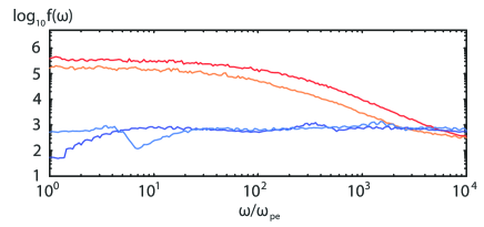
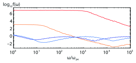
Figure 5: Spectra obtained from jet and ambient electrons for the two viewing angles for $\gamma=15$ (upper) and $\gamma=100$ (lower). Spectra with jet electrons are shown in red ($0^{\circ}$) and orange ($5^{\circ}$). Spectra from ambient electrons show the lowest levels by blue ($0^{\circ}$) and light blue ($5^{\circ}$).

The spectra shown in Fig. 5 are obtained for emission from jet electrons and ambient electrons separately for two case with $\gamma=15{\rm and}100$. In this case the spectra are calculated for head-on radiation ($0^{\circ}$) and $5^{\circ}$. It is noted that In the case with $\gamma=100$ spectrum is extended in the higher frequency. However, the spectrum with viewing angle $5^{\circ}$ is greatly decreased in particular in the high frequency due to the narrow beaming angle.

The radiation from jet electrons show Bremsstrahlung-like spectra as a red line ($0^{\circ}$) and orange line ($5^{\circ}$)  hedeT05 . The spectra with jet electrons are different from the spectra shown in Fig. 2c. Since the magnetic fields generated by the Weibel instability are rather weak and the jet electrons are not much accelerated, the trajectories of jet electrons are almost straight with only a slight bent.

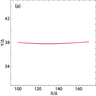
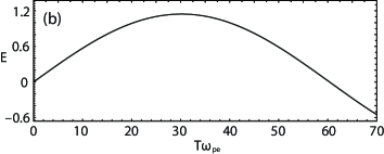
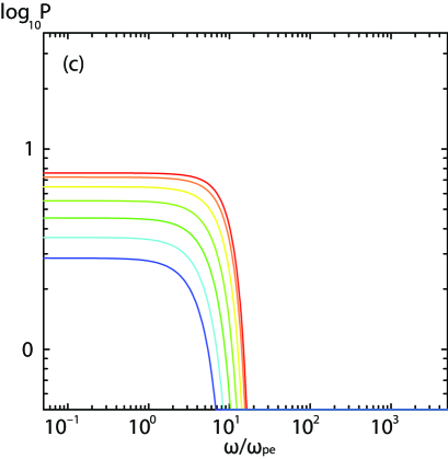
Figure 6: The case with a weak magnetic field ($B_{\rm x}=0.37$) and small perpendicular velocity ($v_{\perp 1}=0.01c,v_{\perp 2}=0.012c$). The paths of two electrons moving helically along the $x-$direction in a homogenous magnetic field shown in the $x-y$-plane (a). The two electrons radiate a time dependent electric field. An observer situated at great distance along the n-vector sees the retarded electric field from the moving electrons (b). The observed power spectrum at different viewing angles from the two electrons (c). Frequency is in units of $\omega_{\rm pe}^{-1}$.

We compare these spectra with our known spectra obtained from two (jet) electrons, the case with a parallel magnetic field ($B_{\rm x}=0.37$), and jet velocity of $v_{\rm j1,2}=0.99c$. Two electrons are injected with different perpendicular velocities ($v_{\perp 1}=0.01c,v_{\perp 2}=0.012c$). A maximum Lorenz factor of $\gamma_{\max}=\{(1-(v_{\rm j2}^{2}+v_{\perp 2}^{2})/c^{2}\}^{-1/2}=7.114$ accompanies the larger perpendicular velocity. The critical angle for off-axis radiation $\theta_{\gamma}=180^{\circ}/(\pi\gamma_{\max})$ for this case is 8.05^∘.

Comparing the spectra with Figs. 5 and 6c we find similarities. The lower frequencies have flat spectra and the higher frequencies decrease monotonically. The slope in Fig. 5 is less steep than that in Fig. 6c. This is due to the fact that the spread of Lorenz factors of jet electrons is substantial and the average Lorenz factor is larger as well. As shown in Fig. 7.16 in Hededal’s Ph. D. thesis  hedeT05 , the turbulent magnetic field with the red noise ($\mu=-3$) makes the spectrum shifted toward higher frequencies. This effect is found in Fig. 5

We obtained spectra using several different parameters with jet electrons and ambient magnetic field. However, the strength of the magnetic fields generated by the Weibel instability is small in the region $x/\Delta<500$ ($\epsilon_{\rm B}<0.07$) as shown in Fig. 1b, therefore the spectra for these cases are very similar to Fig. 5. As shown in Fig. 7.12 in Hededal’s Ph. D. thesis  hedeT05 , the trajectories of jet electrons have to be chaotic to produce a jitter-like spectrum as shown in Fig. 7.22.

In order to obtain the spectrum of synchrotron (jitter) emission, we consider an ensemble of electrons selected in the region where the Weibel instability has fully grown and electrons are accelerated in the generated magnetic fields as shown in Fig. 1, which is being investigted.

IV DISCUSSIONS

Emission obtained with the method described above is obtained self-consistently, and automatically accounts for magnetic field structures on small scales responsible for jitter emission. By performing such calculations for simulations with different parameters, we can investigate and compare the different regimes of jitter- and synchrotron-type emission  medv00 ; medv06 . The feasibility of this approach has already been demonstrated  hedeT05 ; hedeN05 , and its implementation is straightforward. Thus, we should be able to address the low frequency GRB spectral index violation of the synchrotron spectrum line of death  medv06 .

Medvedev and Spitkovsky recently showed that electrons may cool efficiently at or near the shock jump and are capable of emitting a large fraction of the shock energy  MS09 . Such shocks are well-resolved in existing PIC simulations; therefore, the microscopic structure can be studied in detail. Since most of the emission in such shocks would originate from the vicinity of the shock, the spectral power of the emitted radiation can be directly obtained from finite-length simulations and compared with observational data.

As shown in Fig. 1, behind the trailing shock the electrons are accelerated and strong magnetic fields are generated. Therefore, this region seems to produce the emission that is observed by satellites. We will calculate more spectra based on our RPIC simulations and compare in detail with Fermi data.

- (1) K.-I. Nishikawa, P. Hardee, G. Richardson, R. Preece, H., Sol, and G.J. Fishman, ApJ 595 (2003) 555.
- (2) L.O. Silva, R.A. Fonseca, J.W. Tonge, J.M. Dawson, W.B. Mori, and M.V. Medvedev, ApJ 596 (2003) L121.
- (3) J.T. Frederiksen, C.B. Hededal, T. Haugbølle, and Å. Nordlund, ApJ 608 (2004) L13.
- (4) K.-I. Nishikawa, P. Hardee, G. Richardson, R. Preece, R., H. Sol, and G.J. Fishman, ApJ 623 (2005) 927.
- (5) C.B. Hededal, and K.-I. Nishikawa, ApJ 623 (2005) L89.
- (6) C.H. Jaroschek, H. Lesch, and R.A. Treumann, ApJ 618 (2005) 822.
- (7) K.-I. Nishikawa, P. Hardee, C.B. Hededal, and G.J. Fishman, ApJ 642 (2006) 1267.
- (8) E. Ramirez-Ruiz, K.-I. Nishikawa, and C.B. Hededal, ApJ 671 (2007) 1877.
- (9) P. Chang, A. Spitkovsky, and J. Arons, ApJ 674 (2008) 378.
- (10) A. Spitkovsky, ApJ 673 (2008) L39.
- (11) M.E. Dieckmann, P K. Shukla, and L.O.C. Drury, ApJ 675 (2008) 586.
- (12) A. Spitkovsky, ApJ 682 (2008) L5.
- (13) L. Sironi, and A. Spitkovsky, ApJ 698 (2009) 1523.
- (14) E.S. Weibel, Phys. Rev. Lett. 2 (1959) 83.
- (15) M.V. Medvedev, and A. Loeb, ApJ 526 (1999) 697.
- (16) K. -I. Nishikawa, J. Niemiec, P. Hardee, M. Medvedev, H. Sol, Y. Mizuno, B. Zhang, M. Pohl, M., Oka, and D.H. Hartmann, ApJ 689 (2009) L10.
- (17) B. Zhang, and P. Meszaros, Int. J. Mod. Phys. A19 (2004) 2385.
- (18) T. Piran, Rev. Mod. Phys. 76 (2005) 1143.
- Piran (2005b) T. Piran, in the proceedings of Magnetic Fields in the Universe, Angra dos Reis, Brazil, Nov. 29-Dec 3, 2004, Ed. E. de Gouveia del Pino, AIPC 784 (2005) 164.
- (20) B. Zhang, Chin. J. Astron. Astrophys. 7 (2007) 1.
- (21) E. Nakar, Phys. Reports 442 (2007) 166.
- (22) A. Achterberg, Y.A. Gallant, J.G. Kirk, and A.X. Guthmann, MNRAS 328 (2001) 393.
- (23) D. C. Ellison, and G.P. Double, Astroparticle Phys. 18 (2002) 213.
- (24) M. Lemoine, G. Pelletier, ApJ 589 (2003) L73.
- (25) J. Niemiec, and M. Ostrowski, ApJ 641 (2006) 984.
- (26) J. Niemiec, M. Ostrowski, and M. Pohl, ApJ 650 (2006) 1020.
- (27) A. Panaitescu, and P. Kumar, ApJ 560 (2001) L49.
- (28) S. A. Yost, F. A. Harrison, R. Sari, and D.A. Frail, ApJ 597 (2003) 459.
- (29) E. Waxman, Plasma Phys. Control. Fusion 48 (2006) B137.
- (30) P. Meszaros, M.J. Rees, and R.A.M.J. Wijers, ApJ 499 (1998) 301.
- (31) R. Sari, T. Piran, and R. Narayan, ApJ 497 (1998) L17.
- (32) P. Meszaros, and M.J. Rees, ApJ 482 (1997) L29.
- (33) T. Piran, Phys. Rep. 314 (1999) 575.
- (34) T. Piran, Phys. Rep. 333 (2000) 529.
- (35) P. Meszaros, ARAA 40 (2002) 137.
- (36) P. Meszaros, Rept. Prog. Phys. 69 (2006) 2259.
- (37) R.D. Preece, M.S. Briggs, R.S. Mallozzi, G.N. Pendleton, W.S. Paciesas, and D.L. Band, ApJ 506 (1998) L23.
- (38) M. V. Medvedev, ApJ 540 (2000) 704.
- (39) M.V. Medvedev, ApJ 637 (2006) 869.
- (40) K.-I. Nishikawa, J. Niemiec, H. Sol, M. Medvedev, B. Zhang, Å. Nordlund, J.T. Frederiksen, P. Hardee, Y, Mizuno, D.H. Hartmann, and G.J. Fishman, in Proc. of The 4th Heidelberg International Symposium on High Energy Gamma-Ray Astronomy, eds. F. A. Aharonian, W. Hofmann, and F. Rieger (AIPC), 1085 (2009) 589.
- (41) C.B. Hededal, Ph.D. thesis, (2005) (arXiv:astro-ph/0506559).
- (42) C.B. Hededal, and Å. Nordlund, ApJL (2005) submitted, (arXiv:astro-ph/0511662).
- (43) G. B. Rybicki, and A.P. Lightman, Radiative Processes in Astrophysics, (John Wiley & Sons, New York, 1979)
- (44) J. D. Jackson, Classical Electrodynamics, (Interscience, Boston, 1999)
- (45) G. Bekefi, Radiative Processes in Plasmas, (John Wiley & Sons, New York, 1966)
- (46) L. D. Landau, and E.M. & Lifshitz, The Classical Theory of Fields, (Elsevier Science & Technology Books, 1980)
- (47) J.L. Martins, S.F. Martins, R.A. Fonseca, and L.O. and Silva, Proc. of SPIE 7359 (2009) 73590V-1.
- (48) L. Sironi, and A. Spitkovsky, ApJ (2009) submitted, (arXiv:0908.3193).
- (49) M.V. Medvedev, and A. Spitkovsky, ApJ 700 (2009) 956.