Minimum magnetic energy theorem predicts Meissner effect in perfect conductors

Abstract

A theorem on the magnetic energy minimum in a perfect, or ideal, conductor is proved. Contrary to conventional wisdom the theorem provides a classical explanation of the expulsion of a magnetic field from the interior of a conductor that loses its resistivity. It is analogous to Thomson’s theorem which states that static charge distributions in conductors are surface charge densities at constant potential since these have minimum energy. This theorem is proved here using a variational principle. Then an analogous result for the magnetic energy of current distributions is proved: magnetic energy is minimized when the current distribution is a surface current density with zero interior magnetic field. The result agrees with currents in superconductors being confined near the surface and indicates that the distinction between superconductors and hypothetical perfect conductors is artificial.

1 Introduction

In the literature on superconductivity a distinction between superconductors and hypothetical perfect conductors is often made. Even though both have zero resistivity, when penetrated by a constant external magnetic field, the superconductor expels the field (the experimentally observed Meissner effect) but, in the corresponding thought experiment, the perfect conductor does not. Here we will prove a theorem on the magnetic energy minimum from which one concludes that energy minimization and expulsion of an external field is the same thing. Therefore, perfect conductors would in fact behave like superconductors in their approach to thermodynamic equilibrium. Of course, perfect conductors that are not superconductors exist only as thought experiments in textbooks. Nevertheless, textbook thought experiments should be correct, and unfortunately this is not the case at the moment.

For simplicity we concentrate here on the basic case of type I superconductors in a field below the critical field. The outline of this article is as follows. We first discuss the historical background that led Meissner and subsequent textbook authors astray. We then present our derivation of the minimum magnetic energy theorem from a variational principle, after some preliminary background on Thomson’s theorem and its derivation. Previous work on the problem is discussed and then an illuminating example is presented in which the energy reduction can be calculated explicitly. After that we briefly discuss the physical mechanism of field expulsion. The conclusions are followed by an Appendix which gives further motivation and explicit solutions for simple systems.

2 Meissner effect, diamagnetism, and field expulsion

In the original 1933 work [1] by Meissner and Ochsenfeld , they stated, without proof, argument, or reference, that it was understandable that a magnetic field would not enter a superconductor, but that the expulsion of a penetrating field at the phase transition to superconductivity was unexpected. Since then it has been stated innumerable times, in textbooks [3, 4, 5, 6] and pedagogical articles [2, 7], that the expulsion of the magnetic field cannot be understood in terms of zero resistivity alone: superconductors are not just perfect conductors. The purpose of this article is to show that this is not correct so we must first introduce the confused and intricate historical context in which the myth arose.

2.1 The Bohr - van Leeuwen theorem

In 1911 Niels Bohr [8], and then in 1921, more thoroughly, van Leeuwen [9], studied magnetism from the point of view of classical statistical mechanics. They reached the conclusion that dia- and paramagnetism could not be explained by classical theory. This, so called, Bohr-van Leeuwen theorem is often discussed in books on the theory of magnetism, in particular by Van Vleck [10], but also in more recent texts [11, 12]. The model assumed by these authors is a system of classical charged particles, with Coulomb interactions, in a constant external magnetic field. The key observation is that the external magnetic field does not do work on charged particles and therefore does not change the energy. Hence no statistical mechanical response. This may seem watertight but there are weaknesses. For example, the statistical equilibrium distribution is not always determined simply by the energy. If there are other conserved phase space quantities, such as angular momentum, they may also influence the distribution [13]. Dubrovskii [14] has criticized the Bohr-van Leeuwen theorem on these grounds. The main problem though is the assumption of a purely external field, and we return to this below. Nevertheless, the theorem is still discussed in the literature [15, 16, 17] from time to time.

2.2 The Larmor precession

There is another, more fundamental, theorem that is in conflict with the Bohr-van Leeuwen theorem. Basic Lagrangian dynamics can be used to show that a system of particles, with the same charge to mass ratio $q/m$, moving in an axially symmetric external potential, will rotate (precess) with the Larmor frequency $\Omega=qB/2mc$, when placed in a weak constant external magnetic field parallel to the axis. This is Larmor’s theorem [18, 19]. It is easy to show that this precession causes a circulating current which produces a magnetic field that screens the external field [20]. This in accordance with Lenz law and is the basis of Langevin’s classical derivation of diamagnetism. Feynman et al. [21] are aware of this discrepancy and indicate that the Bohr-van Leeuwen result should not be applied to systems that are free to rotate.

2.3 The Fock-Darwin Hamiltonian

The story is, however, even more complicated. A lot of thought has gone into understanding the physics behind the Bohr-and Leeuwen theorem. After all, the external field makes free charged particles circulate with the cyclotron frequency $\omega=qB/mc$, twice the Larmor frequency. Towards the edges of the system this should give rise to a net current. It was then realized that the forces (or the wall) confining the system has the effect of producing a counter current around the edge that cancels this edge effect. The exact canceling of the diamagnetic effect by the edge current, however, contradicts Larmor’s theorem, so the situation is a bit confusing. More detailed studies of these effects have been made using the model system of independent charged particles confined axially by a parabolic potential in a constant external field parallel to the axis. The Hamiltonian for this model is called the Fock-Darwin Hamiltonian [22, 23]. In recent years it has been applied to quantum dots.

One notes that the complete diamagnetism of superconductors is in conflict with the Bohr-van Leeuwen theorem, but not with Larmor’s theorem. In 1938 Welker [24] showed, quantum mechanically, that in a free electron gas, confined in a cylinder, the diamagnetic contribution from Larmor rotation currents is precisely canceled by the paramagnetic effect on the magnetic moments due to orbital angular momenta. This fact led Welker to predict an energy gap in superconductors since this would freeze the paramagnetic degree of freedom. In spite of all these problems with understanding the complete diamagnetism this aspect did not worry Meissner. After all, all metals initially exclude an applied magnetic field by appropriate induced eddy currents. Due to resistance these subside, but in ideal conductors they won’t. Only the expulsion of an already present magnetic field at the phase transition was therefore considered unexpected by Meissner and Ochsenfeld.

2.4 The Darwin Hamiltonian

We note that the findings from the Bohr-van Leeuwen theorem, the Fock-Darwin Hamiltonian, and even Larmor’s theorem, are not relevant to large systems of charged particles. The reason is that considering only an external magnetic field is wrong. Unless the charged particles are all at rest they will be sources of magnetic fields as they move. When there are many particles this effect, which necessarily is small in few-body systems, easily becomes very large [25, 26, 27, 28]. For realistic results one must therefore include the internal magnetic effects in the relevant dynamics. This was first done by Darwin [29]. The Darwin Lagrangian and corresponding Hamiltonian can be used to obtain good quantitative understanding of the complete diamagnetism, as well as the related effect of rotation called the London moment [30].

2.5 Thermodynamics and expulsion

Already in 1934 Gorter and Casimir [31] made a thorough analysis of superconductors from the point of view of classical thermodynamics. One result of these studies is that the flux expulsion is necessary if the superconducting state is to be a thermal equilibrium state. If the final situation depends on which order the phase transition and the external magnetic field appeared one would have a case of hysteresis, the system would remember its past. From this point of view flux expulsion is a natural consequence of approach to thermal equilibrium.

This, of course, does not in itself reveal the actual physical mechanism of the expulsion. This is not a subject that has been much discussed in the literature with the notable exception of Hirsch. In a number of papers Hirsch (see e.g. [32, 33, 34, 35]) speculates on the physical mechanism, and points out that the expulsion is not explained by BCS theory. Forrest [2] argues that conservation of flux through an ideal current loop, as well as plasma physics results on the freezing-in of magnetic field lines, prove that classical electromagnetism cannot explain the expulsion. This will be refuted below.

3 Energy minimum theorems

Electromagnetic energy can be written in a number of different ways. Here we will assume that there are no microscopic dipoles so that distinguishing between the $\mbox{\boldmath$D$},\mbox{\boldmath$H$}$ and $\mbox{\boldmath$E$},\mbox{\boldmath$B$}$ fields is unnecessary. That this is valid when treating the Meissner effect in type I superconductors is stressed by Carr [36]. Relevant energy expressions are then,

$$E_{\rm e}+E_{\rm m} = \frac{1}{8\pi}\!\int(\mbox{\boldmath$E$}^{2}+\mbox{\boldmath$B$}^{2}){\rm d}V$$ (1)

$$= \frac{1}{2}\int\left(\varrho\phi+\frac{1}{c}\mbox{\boldmath$j$}\cdot\mbox{\boldmath$A$}\right){\rm d}V=$$ (2)

$$= \frac{1}{2}\int\!\!\int\left(\frac{\varrho(\mbox{\boldmath$r$})\varrho(\mbox{\boldmath$r$}^{\prime})+\frac{1}{c^{2}}\mbox{\boldmath$j$}(\mbox{\boldmath$r$})\cdot\mbox{\boldmath$j$}(\mbox{\boldmath$r$}^{\prime})}{|\mbox{\boldmath$r$}-\mbox{\boldmath$r$}^{\prime}|}\right){\rm d}V{\rm d}V^{\prime}.$$ (3)

Here the first form is generally valid while the two following assume quasi statics, i.e. essentially negligible radiation.

According to Thomson’s theorem, given a certain number of conductors, each one with a given charge, the charges distribute themselves on the conductor surfaces in order to minimize the electrostatic energy [37]. Even though J. J. Thomson did not present a formal mathematical proof for his result, the proof of the theorem may be found with great detail in [38, 39, 40] and also on its differential form in [41]. A different approach not found in the literature, based on the variational principle, is presented here. Thomson’s result is widely known and has turned to be very useful when applied in several distinct situations. For instance, it was used to determine the induced surface density [42], and in the tracing and the visualization of curvilinear squares field maps [41]. Other applications range from interesting teaching tools [43] to useful computational methods such as Monte Carlo energy minimization [44].

For resistive media currents and magnetic fields always dissipate but for perfect conductors we will here prove an analogous theorem for the magnetic field: The magnetic field energy is minimized by surface current distributions such that the magnetic field is zero inside the perfectly conducting bodies, and the vector potential is parallel to their surfaces. Since energy conservation is assumed, it is clearly only valid for ideal conductors; otherwise steady current exist only if there is an electric field. Previously similar result have appeared in the literature [45, 46] and we discuss those below.

3.1 Thomson’s theorem

In equilibrium, the electrostatic energy functional for a system of conductors surrounded by vacuum, may be written as,

$$E_{\rm e}=\int_{V}\left[\varrho\phi-{1\over 8\pi}\left(\nabla\phi\right)^{2}\right]{\rm d}V,$$ (4)

by combining the electric parts of (1) and (2) and using $\mbox{\boldmath$E$}=-\nabla\phi$. We now split the integration region into the volume of the conductors, $V_{\rm{in}}$, the exterior volume, $V_{\rm{out}}$, and the boundary surfaces $S$,

$$E_{\rm e}=\int_{V_{\rm{in}}}\left[\varrho\phi-{1\over 8\pi}\left(\nabla\phi\right)^{2}\right]{\rm d}V-\int_{V_{\rm{out}}}{1\over 8\pi}\left(\nabla\phi\right)^{2}{\rm d}V+\int_{S}\sigma\phi\,{\rm d}S,$$ (5)

where $\sigma$ is the surface charge distribution.

We now use, $(\nabla\phi)^{2}=\nabla\cdot(\phi\nabla\phi)-\phi\nabla^{2}\phi$, and rewrite the divergencies using Gauss theorem. The energy functional then becomes,

$$E_{\rm e}=\int_{V_{\rm{in}}}\left[\varrho\phi+{1\over 8\pi}\phi\,\nabla^{2}\phi\right]{\rm d}V-\int_{V_{\rm{out}}}{1\over 8\pi}\phi\,\nabla^{2}\phi\,{\rm d}V$$

$$+\int_{S}\left[\sigma\phi-{1\over 8\pi}\phi\,\hat{n}\cdot\left(\nabla^{+}\phi-\nabla^{-}\phi\right)\right]\,{\rm d}S,$$ (6)

where $\nabla^{+}$ and $\nabla^{-}$ are the gradient operators at the surface in the outer and inner limits, respectively. Since the total charge in the conductor is limited and constrained to the conductor volume and surface, one must include this restriction by introducing a Lagrange multiplier $\lambda$. Therefore the infinitesimal variation of the energy is,

$$\delta E_{\rm e} = \int_{V_{\rm{in}}}\left[\delta\phi\left(\varrho+\frac{1}{4\pi}\nabla^{2}\phi\right)+\delta\varrho\left(\phi-\lambda\right)\right]{\rm d}V+\int_{V_{\rm{out}}}\delta\phi\,\frac{1}{4\pi}\nabla^{2}\phi\;{\rm d}V$$ (7)

$$+\int_{S}\left\{\delta\phi\left[\sigma+\frac{1}{4\pi}\hat{n}\cdot\left(\nabla^{+}\phi-\nabla^{-}\phi\right)\right]+\delta\sigma\left(\phi-\lambda\right)\right\}\,{\rm d}S.$$

From this energy minimization, the Euler-Lagrange equations become:

$$V_{\rm{in}}\left\{\begin{array}[]{l}\nabla^{2}\phi=-4\pi\varrho\\ \phi=\lambda\\ \end{array}\right.$$ (8)

$$S\,\,\,\,\left\{\begin{array}[]{l}\sigma=-\frac{1}{4\pi}\hat{n}\cdot\left(\nabla^{+}\phi-\nabla^{-}\phi\right)\\ \phi=\lambda\\ \end{array}\right.$$ (9)

$$V_{\rm{out}}\hskip 14.22636pt\nabla^{2}\phi=0$$ (10)

According to these equations the potential is constant inside the conductor in the minimum energy state. This means the electric charge distribution is on the surface and in an equipotential configuration. This concludes the proof of Thomson’s theorem.

3.2 Minimum magnetic energy theorem

A similar procedure will now be applied to the magnetic field. We write the magnetic energy functional for a time independent magnetic field is written as,

$$E_{\rm m}=\int_{V}\left[\frac{1}{c}\mbox{\boldmath$j$}\cdot\mbox{\boldmath$A$}-{1\over 8\pi}\left(\nabla\times\mbox{\boldmath$A$}\right)^{2}\right]{\rm d}V,$$ (11)

i.e. as two times the form (2) of the magnetic energy minus the form (1), using $\mbox{\boldmath$B$}=\nabla\times\mbox{\boldmath$A$}$. As before we split the volume into the volume interior to conductors, the exterior vacuum, and the surface at the interfaces, and write,

$$E_{\rm m} = \int_{V_{\rm{in}}}\left[\frac{1}{c}\mbox{\boldmath$j$}\cdot\mbox{\boldmath$A$}-{1\over 8\pi}\left(\nabla\times\mbox{\boldmath$A$}\right)^{2}\right]{\rm d}V$$ (12)

$$-\int_{V_{\rm{out}}}{1\over 8\pi}\left(\nabla\times\mbox{\boldmath$A$}\right)^{2}{\rm d}V+\frac{1}{c}\int_{S}\mbox{\boldmath$k$}\cdot\mbox{\boldmath$A$}\,{\rm d}S,$$

where $k$ is the surface current density. We now use the identity,

$$\left(\nabla\times\mbox{\boldmath$A$}\right)^{2}=\nabla\cdot\left[\mbox{\boldmath$A$}\times\left(\nabla\times\mbox{\boldmath$A$}\right)\right]+\mbox{\boldmath$A$}\cdot\left[\nabla\times\left(\nabla\times\mbox{\boldmath$A$}\right)\right],$$ (13)

and then use Gauss theorem to rewrite the divergence terms. The energy functional then becomes:

$$E_{\rm m} = \int_{V_{\rm{in}}}\left\{\frac{1}{c}\mbox{\boldmath$j$}\cdot\mbox{\boldmath$A$}-{1\over 8\pi}\mbox{\boldmath$A$}\cdot\left[\nabla\times\left(\nabla\times\mbox{\boldmath$A$}\right)\right]\right\}{\rm d}V$$

$$-\int_{V_{\rm{out}}}{1\over 8\pi}\mbox{\boldmath$A$}\cdot\left[\nabla\times\left(\nabla\times\mbox{\boldmath$A$}\right)\right]{\rm d}V$$

$$+\int_{S}\left\{\frac{1}{c}\mbox{\boldmath$k$}\cdot\mbox{\boldmath$A$}-{1\over 8\pi}\mbox{\boldmath$A$}\cdot\left[\hat{n}\times\left(\nabla^{+}\times\mbox{\boldmath$A$}-\nabla^{-}\times\mbox{\boldmath$A$}\right)\right]\right\}\,{\rm d}S.$$

As in the electric field case, some constraints should be imposed. In particular, due to charge conservation, the electric current must obey the continuity equation both in volume and at the surface [47]:

$$\nabla\cdot\mbox{\boldmath$j$} = 0$$ (15)

$$\nabla_{S}\cdot\mbox{\boldmath$k$} = 0$$ (16)

where $\nabla_{S}$ is the surface gradient operator. Notice that the constraints are local, not global. In other words, the Lagrange multiplier is not constant but a space function $\lambda(\mbox{\boldmath$r$})$. Therefore, infinitesimal variation of the magnetic energy gives,

$$c\,\delta E_{\rm m}=\int_{V_{\rm{in}}}\left\{\delta\mbox{\boldmath$A$}\cdot\left(\mbox{\boldmath$j$}-\frac{c}{4\pi}\left[\nabla\times\left(\nabla\times\mbox{\boldmath$A$}\right)\right]\right)+\delta\mbox{\boldmath$j$}\cdot\left(\mbox{\boldmath$A$}-\nabla\lambda\right)\right\}{\rm d}V$$

$$-\int_{V_{\rm{out}}}\delta\mbox{\boldmath$A$}\cdot\frac{c}{4\pi}\left[\nabla\times\left(\nabla\times\mbox{\boldmath$A$}\right)\right]{\rm d}V$$ (17)

$$+\int_{S}\left\{\delta\mbox{\boldmath$A$}\cdot\left[\mbox{\boldmath$k$}+\frac{c}{4\pi}\hat{n}\times\left(\nabla^{+}\times\mbox{\boldmath$A$}-\nabla^{-}\times\mbox{\boldmath$A$}\right)\right]+\delta\mbox{\boldmath$k$}\cdot\left(\mbox{\boldmath$A$}-\nabla_{S}\lambda\right)\right\}\,{\rm d}S.$$

Equating this to zero we find that,

$$V_{\rm{in}}\,\,\left\{\begin{array}[]{l}\nabla\times\left(\nabla\times\mbox{\boldmath$A$}\right)=\nabla\times\mbox{\boldmath$B$}=\frac{4\pi}{c}\mbox{\boldmath$j$}\;,\\ \mbox{\boldmath$A$}=\nabla\lambda\;,\\ \end{array}\right.$$ (18)

and,

$$S\,\,\,\,\left\{\begin{array}[]{l}\mbox{\boldmath$k$}=\frac{c}{4\pi}\hat{n}\times\left(\nabla^{+}\times\mbox{\boldmath$A$}-\nabla^{-}\times\mbox{\boldmath$A$}\right)\;,\\ \mbox{\boldmath$A$}=\nabla_{S}\lambda\;,\\ \end{array}\right.$$ (19)

and,

$$V_{\rm{out}}\;\;\;\nabla\times\left(\nabla\times\mbox{\boldmath$A$}\right)=\nabla\times\mbox{\boldmath$B$}=0,$$ (20)

are the Euler-Lagrange equations for this energy functional.

According to eq. (18) $\mbox{\boldmath$B$}=\nabla\times\nabla\lambda=\mbox{\boldmath$0$}$, so the magnetic field must be zero in $V_{\rm{in}}$. Consequently also the volume current density is zero, $\mbox{\boldmath$j$}=\mbox{\boldmath$0$}$, inside the conductor, in the minimum energy state.

3.2.1 Surface currents

Now consider the results for the surface, eq. (19). Our results from $V_{\rm{in}}$ show that $\nabla^{-}\times\mbox{\boldmath$A$}=\mbox{\boldmath$0$}$, so the equation reads,

$$\mbox{\boldmath$k$}=\frac{c}{4\pi}\hat{n}\times\left(\nabla^{+}\times\nabla_{S}\lambda\right).$$ (21)

Let us introduce a local Cartesian coordinate system with origin on the surface, such that the surface is spanned by $\hat{x},\hat{y}$ with unit normal $\hat{n}=\hat{z}=\hat{x}\times\hat{y}$. Assuming that the surface is approximately flat we then have that,

$$\nabla_{S}=\hat{x}\frac{\partial}{\partial x}+\hat{y}\frac{\partial}{\partial y},\;\;\mbox{and,}\;\;\nabla^{+}=\hat{x}\frac{\partial}{\partial x}+\hat{y}\frac{\partial}{\partial y}+\hat{n}\frac{\partial}{\partial z^{+}}=\nabla_{S}+\hat{n}\frac{\partial}{\partial z^{+}}.$$ (22)

Since, $\mbox{\boldmath$A$}=\nabla_{S}\lambda$, the vector potential is tangent to the conducting surface and we get,

$$\displaystyle\frac{4\pi}{c}\mbox{\boldmath$k$}=\hat{n}\times\left[\left(\nabla_{S}+\hat{n}\frac{\partial}{\partial z^{+}}\right)\times\nabla_{S}\lambda(x,y,z)\right]$$ (23)

$$\displaystyle=\hat{n}\times\left[\hat{n}\frac{\partial}{\partial z^{+}}\times\left(\hat{x}\frac{\partial\lambda}{\partial x}+\hat{y}\frac{\partial\lambda}{\partial y}\right)\right]=\hat{n}\times\left(\hat{n}\frac{\partial}{\partial z^{+}}\times\mbox{\boldmath$A$}\right),$$ (24)

for the surface current density. Rewriting the triple vector product we find,

$$\frac{4\pi}{c}\mbox{\boldmath$k$}=\frac{\partial}{\partial z^{+}}\left[(\hat{n}\cdot\mbox{\boldmath$A$})\hat{n}-(\hat{n}\cdot\hat{n})\mbox{\boldmath$A$}\right]=-\frac{\partial\mbox{\boldmath$A$}}{\partial z^{+}}.$$ (25)

so the surface current density is parallel to the outside normal derivative of the vector potential. We note that this agree with the well known result [40],

$$\frac{4\pi}{c}\mbox{\boldmath$k$}=\hat{n}\times(\mbox{\boldmath$B$}_{+}-\mbox{\boldmath$B$}_{-})$$ (26)

for the case of zero interior field ($\mbox{\boldmath$B$}_{-}=\mbox{\boldmath$0$}$).

3.2.2 External fields

Even though the proof of the theorem does not include the presence of an external magnetic field, the result can be generalized. Assume that the magnetic field is produced by currents at infinity. These currents demand a non-zero surface integral at infinity in eq. (3.2) which does not affect the final result, however. Alternatively one can include large perfectly conducting Helmholtz coils (tori) in the system and let the rest of the system be small and situated in the constant field region of the coils. In section 4 we instead treat this case by means of an illuminating example.

3.3 Previous work

The fact that there is an energy minimum theorem for the magnetic energy of ideal, or perfect, conductors, analogous to Thomson’s theorem, is not entirely new. In an interesting, but difficult and ignored, article by Karlsson [45] such a theorem is stated. Karlsson, however, restricts his theorem to conductors with holes in them. In the electrostatic case charge conservation prevents the energy minimum from being the trivial zero field solution. In the magnetic ideal conductor case a corresponding conservation law is the conservation of magnetic flux through a hole [48]. But, as long as one conductor of the system has a hole with conserved flux there will be a non-trivial magnetic field. To require that all conductors of the system have holes, as Karlsson does, seems to us unnecessarily restrictive. One of his main results is that a the current distribution on a superconducting torus minimizes the magnetic energy.

A result by Badía-Majós [46] comes even closer to our own and we outline it here. The current density is assumed to be of the form,

$$\mbox{\boldmath$j$}=qn\mbox{\boldmath$v$},$$ (27)

where $q$ is the charge of the charge carriers and $n$ is their number density. The time derivative is then given by,

$$\frac{{\rm d}\mbox{\boldmath$j$}}{{\rm d}\,t}=\frac{qn}{m}\,m\frac{{\rm d}\mbox{\boldmath$v$}}{{\rm d}\,t}=\frac{qn}{m}\left(q\mbox{\boldmath$E$}+\frac{q}{c}\mbox{\boldmath$v$}\times\mbox{\boldmath$B$}\right)=\frac{q^{2}n}{m}\mbox{\boldmath$E$}+\frac{q}{mc}\mbox{\boldmath$j$}\times\mbox{\boldmath$B$},$$ (28)

assuming that only the Lorentz force acts (ideal conductor). We now recall Poynting’s theorem [19] for the time derivative of the field energy density of a system of charged particles,

$$\frac{{\rm d}}{{\rm d}\,t}\left(\frac{\mbox{\boldmath$E$}^{2}+\mbox{\boldmath$B$}^{2}}{8\pi}\right)=-\mbox{\boldmath$j$}\cdot\mbox{\boldmath$E$}-\nabla\cdot\left(\frac{c}{4\pi}\mbox{\boldmath$E$}\times\mbox{\boldmath$B$}\right).$$ (29)

The first term on the right hand side normally represents resistive energy loss. Here we use the result for $E$ from eq. (28),

$$\mbox{\boldmath$E$}=\frac{m}{q^{2}n}\frac{{\rm d}\mbox{\boldmath$j$}}{{\rm d}\,t}-\frac{1}{qnc}\mbox{\boldmath$j$}\times\mbox{\boldmath$B$},$$ (30)

and get,

$$\mbox{\boldmath$j$}\cdot\mbox{\boldmath$E$}=\frac{m}{q^{2}n}\,\frac{{\rm d}\mbox{\boldmath$j$}}{{\rm d}\,t}\cdot\mbox{\boldmath$j$}=\frac{{\rm d}}{{\rm d}\,t}\left(\frac{m}{2q^{2}n}\mbox{\boldmath$j$}^{2}\right).$$ (31)

This is thus the natural form for this term for perfect conductors. We insert it into (29), neglect radiation, and assume that $\mbox{\boldmath$E$}^{2}\ll\mbox{\boldmath$B$}^{2}$. This gives us,

$$\frac{{\rm d}}{{\rm d}\,t}\left(\frac{1}{8\pi}\mbox{\boldmath$B$}^{2}+\frac{m}{2q^{2}n}\mbox{\boldmath$j$}^{2}\right)=0.$$ (32)

Finally inserting, $\mbox{\boldmath$j$}=(c/4\pi)\nabla\times\mbox{\boldmath$B$}$, here, gives,

$$E_{B}=\frac{1}{8\pi}\left[\int_{V}\mbox{\boldmath$B$}^{2}{\rm d}V+\int_{V_{\rm{in}}}\frac{mc^{2}}{4\pi q^{2}n}(\nabla\times\mbox{\boldmath$B$})^{2}{\rm d}V\right],$$ (33)

for the conserved energy, after integration over space and time.

Badía-Majós [46] then notes that this energy functional implies flux expulsion from superconductors. Variation of the functional gives the London equation [49],

$$\mbox{\boldmath$B$}+\frac{1}{4\pi}\frac{mc^{2}}{q^{2}n}\nabla\times(\nabla\times\mbox{\boldmath$B$})=\mbox{\boldmath$0$}.$$ (34)

Badía-Majós, however, does not point out that this classical derivation of flux expulsion is in conflict with text book statements to the effect that no such classical result exists. Further work by Badía-Majós et al. [50] on variational principles for electromagnetism in conducting materials should be noted.

4 Ideally conducting sphere in external field

We now know that magnetic energy minimum occurs when current flows only on the surface and the magnetic field is zero inside. Let us consider a perfectly conducting sphere in a fixed constant external magnetic field. Here we will calculate the surface current needed to exclude the magnetic field from the interior and how much the energy is then reduced. In order to exclude a constant external field $B$ from its interior the currents on the sphere must obviously produce an interior magnetic field $-\mbox{\boldmath$B$}$, thereby making the total field zero in the interior. It is well known that a constant field is produced inside a sphere by a current distribution represented by the rigid rotation of a constant surface charge density.

4.1 Energy of the external field

For the total magnetic field to have a finite energy we can not assume that the constant external field extends to infinity. Instead of using Helmholtz coils we simplify the mathematics and produce our external field by a spherical shell of current that is equivalent to a rigidly rotating current distribution on the surface. This can be done in practice by having as set of rings representing closely spaced longitudes on a globe with the right amount of currents maintained in each of them. Such a spherical shell of rigidly rotating charge produces a magnetic field that is constant inside the sphere and a pure dipole field outside the sphere (see Fig. 1):

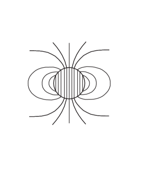
Figure 1: The field lines of the field of Eq. (35) for a nonmagnetic sphere with a rigidly rotating homogeneous surface charge density.

$$\mbox{\boldmath$B$}(\mbox{\boldmath$r$})=\left\{\begin{array}[]{ll}\displaystyle\frac{2\mbox{\boldmath$m$}}{R^{3}}&\mbox{for $r\leq R$}\\ &\mbox{ }\\ \displaystyle\frac{3(\mbox{\boldmath$m$}\cdot\hat{r})\hat{r}-\mbox{\boldmath$m$}}{r^{3}}&\mbox{for $r>R$}\end{array}\right.$$ (35)

Here $r=|\mbox{\boldmath$r$}|$ and the center of the sphere is at the origin. If $Q$ is the total rotating surface charge and $\omega$ its angular velocity,

$$\mbox{\boldmath$m$}=\frac{QR^{2}}{3c}\mbox{\boldmath$\omega$},$$ (36)

see eq. (54) below. It is now easy to calculate the magnetic energy of this field. One finds,

$$E_{0}=\frac{1}{8\pi}\left(\int_{r<R}\mbox{\boldmath$B$}^{2}{\rm d}V+\int_{r>R}\mbox{\boldmath$B$}^{2}{\rm d}V\right)=\left(\frac{2}{3}+\frac{1}{3}\right)\frac{\mbox{\boldmath$m$}^{2}}{R^{3}}=\frac{m^{2}}{R^{3}}.$$ (37)

Inside this sphere, which is assumed to maintain a constant magnetic field in its interior, we now place a smaller perfectly conducting sphere.

4.2 Magnetic energy of the two sphere system

We assume that the small sphere in the middle of the big one has radius $a<R$ and that it also produces a magnetic field by a rigidly rotating charged shell on its surface. We denote its dipole moment by $\mbox{\boldmath$m$}_{a}$ so that its total energy would be,

$$E_{a}=\frac{\mbox{\boldmath$m$}_{a}^{2}}{a^{3}}=\frac{m_{a}^{2}}{a^{3}},$$ (38)

far from all other fields, according to our previous result (37). We now place the small sphere inside the large one and assume that $\mbox{\boldmath$m$}_{a}$ makes an angle $\alpha$ with $m$,

$$\mbox{\boldmath$m$}\cdot\mbox{\boldmath$m$}_{a}=m\,m_{a}\cos\alpha.$$ (39)

The total energy of the system is now,

$$E=\frac{1}{8\pi}\int(\mbox{\boldmath$B$}+\mbox{\boldmath$B$}_{a})^{2}{\rm d}V=E_{0}+E_{a}+E_{i},$$ (40)

where the interaction energy is,

$$E_{i}=\frac{1}{4\pi}\int\mbox{\boldmath$B$}\cdot\mbox{\boldmath$B$}_{a}{\rm d}V$$ (41)

The integral here must be split into the three radial regions: $0\leq r<a$, $a\leq r<R$, and $R\leq r$. The calculations are elementary using spherical coordinates. The contribution from the inner region is

$$E_{i1}=\frac{1}{4\pi}\int_{r<a}\mbox{\boldmath$B$}\cdot\mbox{\boldmath$B$}_{a}{\rm d}V=\frac{4}{3}\frac{mm_{a}}{R^{3}}\cos\alpha$$ (42)

The middle region where there is a dipole field from the small sphere in the constant field from the big one contributes zero: $E_{i2}=0$. The outer region gives $E_{i3}=(2/3)mm_{a}\cos\alpha/R^{3}$. Summing up one finds,

$$E_{i}=2\frac{mm_{a}}{R^{3}}\cos\alpha,$$ (43)

for the magnetic interaction energy of the two spheres.

4.3 Minimizing the total magnetic energy

The total magnetic energy of the system discussed above is thus,

$$E_{0}+E_{a}+E_{i}=E(m_{a},\alpha)=\frac{m^{2}}{R^{3}}+\frac{m_{a}^{2}}{a^{3}}+2\frac{mm_{a}}{R^{3}}\cos\alpha.$$ (44)

We assume that $m$ and $m_{a}$ are positive quantities. This means that as a function of $\alpha$ this quantity is guarantied to have its minimum when $\cos\alpha=-1$, i.e. for $\alpha=\pi$. Thus, at minimum, the dipole of the inner sphere has the opposite direction to that of the constant external field.

Now assuming $\alpha=\pi$ we can look for the minimum as a function of $m_{a}$. Elementary algebra shows that this minimum is attained for,

$$m_{a}=\left(\frac{a}{R}\right)^{3}m\,\equiv m_{\rm min}.$$ (45)

The magnetic field in the interior of the inner sphere is then,

$$\mbox{\boldmath$B$}+\mbox{\boldmath$B$}_{a}=\frac{2\mbox{\boldmath$m$}}{R^{3}}+\frac{2\mbox{\boldmath$m$}_{a}}{a^{3}}=\left(\frac{2m}{R^{3}}-\frac{2m_{\rm min}}{a^{3}}\right)\frac{\mbox{\boldmath$m$}}{m}=\mbox{\boldmath$0$},$$ (46)

so it has been expelled. The minimized energy (44) of the system is found to be,

$$E_{\rm min}=E(m_{\rm min},\pi)=\frac{m^{2}}{R^{3}}\left[1-\left(\frac{a}{R}\right)^{3}\right].$$ (47)

The relative energy reduction is thus given by the volume ratio of the two spheres. Using $\mbox{\boldmath$B$}=2\mbox{\boldmath$m$}/R^{3}$ from (35) the energy lowering can also be expressed as follows:

$$E_{0}-E_{\rm min}=\frac{m^{2}}{R^{3}}\frac{a^{3}}{R^{3}}=\frac{\mbox{\boldmath$B$}^{2}}{4}a^{3}=3\left(\frac{\mbox{\boldmath$B$}^{2}}{8\pi}\right)\left(\frac{4\pi a^{3}}{3}\right).$$ (48)

This result is independent of the radius of the big sphere introduced to produce the constant external field. It shows that the energy lowering corresponds to three times the external magnetic energy in the volume $4\pi a^{3}/3$ of the perfectly conducting sphere.

5 The mechanism of flux expulsion

Assume that a resistive metal sphere is penetrated by a constant magnetic field. Lower the temperature until the resistance vanishes. How does the metal sphere expel the magnetic field, or equivalently, how does it produce surface currents that screen the external field? According to Forrest [2] this can not be understood from the point of view of classical electrodynamics since in a perfectly conducting medium the field lines must be frozen-in. This claim is motivated thus: When the resistivity is zero there can be no electric field according to Ohm’s law, since this law then predicts infinite current. But if the electric field is zero the Maxwell equation, $\nabla\times\mbox{\boldmath$E$}-\partial\mbox{\boldmath$B$}/\partial\,t=\mbox{\boldmath$0$}$, requires that the time derivative of the magnetic field is zero. Hence it must be constant.

Ohm’s law is, however, hardly applicable in this situation. The system of charged particles undergoes thermal fluctuations and these produce electric and magnetic fields. The electric fields accelerate charges according to the Lorentz force law. In the normal situation these currents stay microscopic. When there is an external magnetic field present the overall energy is lowered if these microscopic currents correlate and grow to exclude the external field. According to standard statistical mechanics the system will eventually relax to the energy minimum state consistent with constraints. We note that Alfvén and Fälthammar [51] state that ”in low density plasmas the concept of frozen-in lines of force is questionable”.

Another argument by Forrest [2] is that the magnetic flux through a perfectly conducting current loop is conserved. Since one can imagine arbitrary current loops in the metal that just lost its resistivity with a magnetic field inside, the field must remain fixed, it seems. Is is indeed correct that the flux through ideal current loops is conserved, but the actual physical current loop will not remain intact unless constrained by non-electromagnetic forces. On a loop of current that encloses a magnetic flux there will be forces that expand it [40]. This is the well know mechanism behind the rail gun, see e.g. Essén [52]. All the little current loops in the metal will thus expand until they come to the surface where the expansion stops. In this way the interior field is thinned out and current concentrates near the surface. So, the flux is conserved through the loops, but the loops expand.

6 Conclusions

We have now reached the conclusion that the Meissner effect, both the perfect diamagnetism and the flux expulsion, are consequences of classical electrodynamics, together with reasonable assumptions about the system of charged particles. The reason that this has not been recognized before is a widespread ignorance of the properties and effects of the magnetic interaction energy between moving charged particles. The majority of the physics community tends to think of magnetism as either due to microscopic dipoles in a medium or as due to an imposed external magnetic field. That the translational motion of the charged particles of the system also produces magnetic fields, which in turn change their motion, is normally neglected. When this can not be neglected one must find a self consistent simultaneous solution for currents and magnetic fields [53]. More awareness of these facts will hopefully clear up a lot of confusion in the future.

Appendix A Appendix

A.1 Magnetic energy minimization in simple one degree of freedom model systems

We now define simple one degree of freedom model systems and use them to illustrate how the minimum magnetic energy theorem works. We take systems in which all energies can be calculated exactly so that energy minimization amounts to minimizing a function of a single variable. The systems are both related to a system used by Brito and Fiolhais [43] to study electric energy.

A.1.1 Magnetic energy of coaxial cable

The minimum magnetic energy theorem can be illustrated in such a simple system as a coaxial cable. The cable can be modelled by an outer cylindrical conducting shell with radius $b$, carrying an electric current $I$, and a concentric solid cylindrical conductor with radius $a<b$, carrying the same electric current in the opposite direction. We now divide the inner current into a surface current $I_{s}=(1-\eta)I$ at $\rho=a$ and a bulk current $I_{v}=\eta I$ in the inner volume, $0\leq\rho<a$, so that $I=I_{s}+I_{v}$. We use cylindrical coordinates, $\rho,\varphi,z$, and obtain the magnetic field,

$$\mbox{\boldmath$B$}=\frac{2I}{c}\cdot\left\{\begin{array}[]{ll}\displaystyle\frac{\eta\rho}{a^{2}}\,\hat{\varphi}&\;\;0\leq\rho<a\\ &\\ \displaystyle\frac{1}{\rho}\,\hat{\varphi}&\;\;a\leq\rho\leq b\\ &\\ \displaystyle 0&\;\;b<\rho\\ \end{array}\right.$$ (49)

using Ampère’s law. Thus, the magnetic field energy for a length $L$ of the cable is given by:

$$E_{\rm m} = \frac{1}{8\pi}\int_{V}\mbox{\boldmath$B$}^{2}{\rm d}V$$ (50)

$$= \frac{1}{8\pi}\left(\frac{2I}{c}\right)^{2}\left[\int_{0}^{a}\left(\frac{\eta\rho}{a^{2}}\right)^{2}L2\pi\rho\,{\rm d}\rho+\int_{a}^{b}\left(\frac{1}{\rho}\right)^{2}L2\pi\rho\,{\rm d}\rho\right]$$

$$= \frac{LI^{2}}{c^{2}}\left[\frac{\eta^{2}}{4}+\ln\!\left(\frac{b}{a}\right)\right].$$

This magnetic energy reaches its minimum for zero bulk current, $\eta=0$, corresponding to surface current only and zero field for $0\leq\rho<a$.

A.1.2 Current in sphere due to rigidly rotating charge

Consider an ideally conducting sphere of radius $R$. Assume that there is a circulating current in the sphere which can be seen as the rigid rotation of a charge $Q$ evenly distributed in the thick spherical shell between $r=a<R$ and $r=R$. The charge density,

$$\varrho(\mbox{\boldmath$r$})=\left\{\begin{array}[]{ll}\displaystyle 0&\mbox{for $0\leq r<a$}\\ &\mbox{ }\\ \displaystyle\frac{3Q}{4\pi(R^{3}-a^{3})}&\mbox{for $a\leq r\leq R$}\\ &\mbox{ }\\ 0&\mbox{for $R<r$}\end{array}\right.$$ (51)

is assumed to rotate with angular velocity $\mbox{\boldmath$\omega$}=\omega\,\hat{z}$ relative to a an identical charge density of opposite sign at rest. The current density is then,

$$\mbox{\boldmath$j$}(\mbox{\boldmath$r$})=\varrho(\mbox{\boldmath$r$})\,\mbox{\boldmath$\omega$}\times\mbox{\boldmath$r$},$$ (52)

and the current, $I=\frac{Q}{2\pi}\omega,$ passes through a half plane with the $z$- axis as edge.

The vector potential produced by this current density can be found using the methods of Essén [20], see also [25, 28, 30]. If we introduce $\xi=a/R$ we find,

$$\mbox{\boldmath$A$}(\mbox{\boldmath$r$})=\frac{Q}{c}(\mbox{\boldmath$\omega$}\times\mbox{\boldmath$r$})\cdot\left\{\begin{array}[]{ll}\displaystyle\frac{(1-\xi^{2})}{2(1-\xi^{3})R}&\mbox{for $0\leq r<a$}\\ &\mbox{ }\\ \displaystyle\frac{R^{2}}{10(1-\xi^{3})}\left(\frac{5}{R^{3}}-3\frac{r^{2}}{R^{5}}-2\frac{\xi^{5}}{r^{3}}\right)&\mbox{for $a\leq r\leq R$}\\ &\mbox{ }\\ \displaystyle\frac{(1-\xi^{5})}{5(1-\xi^{3})}\frac{R^{2}}{r^{3}}&\mbox{for $R<r$}\end{array}\right.$$ (53)

The parameter $\xi=a/R$ is zero, $\xi=0$, for a homogeneous ball of rotating charge, while $\xi=1$ corresponds to a rotating shell of surface charge. Comparing with the vector potential for a constant field, $\mbox{\boldmath$A$}=\frac{1}{2}\mbox{\boldmath$B$}_{0}\times\mbox{\boldmath$r$}$ we see that,

$$\mbox{\boldmath$B$}_{0}=\frac{Q\mbox{\boldmath$\omega$}}{cR}\frac{(1-\xi^{2})}{(1-\xi^{3})}=\frac{Q\mbox{\boldmath$\omega$}}{cR}\frac{(1+\xi)}{(1+\xi+\xi^{2})}$$ (54)

is the field in the central current free region $0\leq r<a$.

A.1.3 Magnetic energy of rotating spherical shell current

We now calculate the magnetic energy of this system using the formula,

$$E_{m}=\frac{1}{2c}\int\mbox{\boldmath$j$}\cdot\mbox{\boldmath$A$}\;{\rm d}V.$$ (55)

Performing the integration using spherical coordinates gives,

$$E_{m}=\left(\frac{R\omega}{c}\right)^{2}\frac{Q^{2}}{R}\;f(\xi),$$ (56)

where,

$$f(\xi)=\frac{2+4\xi+6\xi^{2}+8\xi^{3}+10\xi^{4}+5\xi^{5}}{35(1+\xi+\xi^{2})^{2}},$$ (57)

is a function of the dimensionless parameter $\xi$.

This expression for the energy is the Lagrangian form of a kinetic energy which depends on the generalized velocity $\omega=\dot{\varphi}$,

$$L_{m}(\dot{\varphi})=\frac{R^{2}}{c^{2}}\frac{Q^{2}}{R}\;f(\xi)\,\dot{\varphi}^{2}.$$ (58)

Since the generalized coordinate $\varphi$ does not appear in the Lagrangian $L_{m}$ the corresponding generalized momentum (the angular momentum),

$$p_{\varphi}=\frac{\partial L_{m}}{\partial\dot{\varphi}}=2\frac{R^{2}}{c^{2}}\frac{Q^{2}}{R}\;f(\xi)\,\dot{\varphi},$$ (59)

is a conserved quantity. The corresponding Hamiltonian form for the energy is then $H_{m}=p_{\varphi}\dot{\varphi}-L_{m}$, expressed in terms of $p_{\varphi}$,

$$H_{m}(p_{\varphi})=\frac{c^{2}}{4}\frac{p_{\varphi}^{2}}{Q^{2}f(\xi)R}.$$ (60)

The function $1/f(\xi)$ is plotted in Fig. 2.

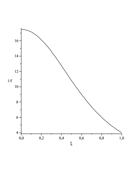
Figure 2: A graph of the function $1/f(\xi)$ which is proportional to the Hamiltonian form of the magnetic energy (60) of our model system. Note that $\xi=0$ corresponds to volume (bulk) current and $\xi=1$ to pure surface current.

We now consider the two energy expressions (58) and (60) separately.

Case of constant current: We first consider the case that the current, $I=Q\omega/2\pi$, is constant. Changing $\xi$ then means changing the conductor geometry while keeping a constant total current, or, equivalently, angular velocity $\omega=\dot{\varphi}$. One might regard the total current as flowing in a continuum of circular wires. Changing $\xi$ from zero to one means changing the distribution of these circular wires from a bulk distribution in the sphere to a pure surface distribution, while maintaining constant current. According to a result by Greiner [54] a system will tend to maximize its magnetic energy when the conductor geometry changes while currents are kept constant. This has also been discussed in Essén [52]. In conclusion, if currents are kept constant the magnetic energy (58) will tend (thermodynamically) to a stable equilibrium with at a maximum value and we note that this corresponds to a pure surface current $\xi=1$.

Case of constant angular momentum: Assume now that we pass to the Hamiltonian (canonical) formalism. Thermodynamically this type of system should tend to minimize its phase space energy (60) in accordance with ordinary Maxwell-Boltzmann statistical mechanics. As a function of $\xi$ this Hamiltonian form of the energy clearly has a minimum at $\xi=1$, see Fig. 2, corresponding to pure surface current. In this case therefore there will be current density only on the surface in the energy minimizing state. This is in accordance with the our minimum magnetic energy theorem. It is notable that both the assumption of constant current and the assumption of constant angular momentum lead to a pure surface current density as the stable equilibrium.

A.2 Explicit solutions with minimum magnetic energy

Here we present two explicit solutions for the current distributions and magnetic fields that minimize the magnetic energy. The solution for a torus has been found several times, probably first by Fock [55], but, independently, several times since then, see e.g. [56, 57, 58, 59, 60, 61], so we do not repeat it here. Karlsson [45], however, was probably the first to notice that the solution minimizes magnetic energy for constant flux. Dolecek and de Launay [48] verified experimentally that a type I superconducting torus behaves exactly as the corresponding classical perfectly diamagnetic system for field strength below the critical field. Here we treat two simpler cases involving constant external fields: a cylinder in a transverse magnetic field, and a sphere.

A.2.1 Cylinder in external perpendicular magnetic field

Consider an infinite cylindrical ideal conductor with radius $R$ in a external constant perpendicular magnetic field. To get the vector potential one must solve the following differential equation,

$$\nabla\times\mbox{\boldmath$B$}=\nabla\times\left(\nabla\times\mbox{\boldmath$A$}\right)=0.$$ (61)

To solve this one should look for the symmetries of the system. We assume that the external constant magnetic field points in the $y$-direction and that the cylinder axis coincides with the $z$-axis. There will then be no dependence on the $z$-coordinate so the magnetic field is,

$$\mbox{\boldmath$B$}=\frac{1}{\rho}\frac{\partial A_{z}}{\partial\varphi}\,\hat{\rho}-\frac{\partial A_{z}}{\partial\rho}\,\hat{\varphi}+\frac{1}{\rho}\left(\frac{\partial}{\partial\rho}(\rho A_{\varphi})-\frac{\partial A_{\rho}}{\partial\varphi}\right)\hat{z}.$$ (62)

Moreover, due to the symmetry of the system, the $z$-component of the magnetic field must be zero,

$$\frac{\partial}{\partial\rho}(\rho A_{\varphi})-\frac{\partial A_{\rho}}{\partial\varphi}=0.$$ (63)

These assumptions and constraints transform eq. (61) into,

$$\nabla\times\mbox{\boldmath$B$}=-\left(\frac{1}{\rho^{2}}\frac{\partial^{2}A_{z}}{\partial\varphi^{2}}+\frac{\partial^{2}A_{z}}{\partial\rho^{2}}+\frac{1}{\rho}\frac{\partial A_{z}}{\partial\rho}\right)\hat{z}=0$$ (64)

which simply is Laplace equation in cylindrical coordinates ($\rho,\varphi,z$). Before writing down the general solution, let’s analyze the boundary conditions. As $\rho\rightarrow\infty$, the magnetic field must approach the external one: $\mbox{\boldmath$B$}_{0}=B_{0}\hat{y}=B_{0}(\hat{\varphi}\cos\varphi+\hat{\rho}\sin\varphi)$. Furthermore, since the magnetic field is zero inside the perfect conductor, one concludes from eq. (62) that the vector potential vector must be constant inside the cylinder. Therefore, the solution is,

$$A_{z}=\textrm{const.}+B_{0}\left(\frac{R^{2}}{\rho}-\rho\right)\cos\varphi,$$ (65)

for $\rho>R$. The magnetic field outside the cylinder becomes,

$$\mbox{\boldmath$B$}=\hat{\rho}\,B_{0}\left(1-\frac{R^{2}}{\rho^{2}}\right)\sin\varphi+\hat{\varphi}\,B_{0}\left(1+\frac{R^{2}}{\rho^{2}}\right)\cos\varphi,$$ (66)

which implies that,

$$\mbox{\boldmath$B$}(\rho=R)=2B_{0}\cos\varphi\,\,\hat{\varphi}$$ (67)

The magnetic field on the cylinder’s surface determines the surface current according to eq. (26), so we get,

$$\mbox{\boldmath$k$}=\frac{c}{2\pi}B_{0}\cos\varphi\,\,\hat{z}.$$ (68)

The total current obtained through integration of the surface current is zero as expected, otherwise the energy would diverge. A more detailed analysis on this problem can be found in [62].

A.2.2 Superconducting sphere in constant magnetic field

Similar calculations can be performed for a superconducting sphere with radius $R$ in a constant external magnetic field pointing in the direction of the $z$-axis.

Similarly to the cylinder case, eq. (61) is simplified a lot due to the symmetries of the system. Since the external constant magnetic field points along the $z$-axis, there won’t be any dependencies on the $\varphi$ coordinate and the magnetic field along this coordinate must be zero. Therefore, the magnetic field simplifies to,

$$\mbox{\boldmath$B$}=\frac{1}{r\sin\theta}\frac{\partial}{\partial\theta}\left(A_{\varphi}\sin\theta\right)\hat{r}-\frac{1}{r}\frac{\partial}{\partial r}\left(A_{\varphi}r\right)\hat{\theta},$$ (69)

where we use spherical coordinates $r,\theta,\varphi$. Again, using these assumptions and constraints eq. (61) becomes,

$$\nabla\times\mbox{\boldmath$B$}=-\frac{1}{r}\left[\frac{\partial}{\partial r}\left(\frac{\partial}{\partial r}\left(rA_{\varphi}\right)\right)+\frac{1}{r}\frac{\partial}{\partial\theta}\left(\frac{1}{\sin\theta}\frac{\partial}{\partial\theta}\left(A_{\varphi}\sin\theta\right)\right)\right]\hat{\varphi}=0$$ (70)

Since the magnetic field is zero inside the sphere, eq. (69) implies that the vector potential has the form,

$$A_{\varphi}(r<R)=\frac{C}{r\sin\theta},$$ (71)

where $C$ is a constant. To prevent the vector potential from diverging at $r=0$ and $\theta=0$, the constant $C$ must be zero. Furthermore, as $r\rightarrow\infty$, the magnetic field must go to the external field, $\mbox{\boldmath$B$}_{0}=B_{0}\hat{z}=B_{0}(\hat{r}\cos\theta-\hat{\theta}\sin\theta)$. Therefore, the solution of eq. (70) for this case is,

$$A_{\varphi}(r>R)=\frac{B_{0}}{2}\left(r-\frac{R^{3}}{r^{2}}\right)\sin\theta,$$ (72)

which leads to the following magnetic field outside the sphere,

$$\mbox{\boldmath$B$}=\hat{r}\,B_{0}\left(1-\frac{R^{3}}{r^{3}}\right)\cos\theta-\hat{\theta}\,B_{0}\left(1+\frac{1}{2}\frac{R^{3}}{r^{3}}\right)\sin\theta.$$ (73)

The magnetic field at the sphere surface is thus,

$$\mbox{\boldmath$B$}=-\frac{3}{2}B_{0}\sin\theta\,\,\hat{\theta}.$$ (74)

One notes that this is the same field as that of section 4.2 at the surface of the inner sphere when energy is minimized.

Using eq. (26), the surface current density becomes,

$$\mbox{\boldmath$k$}=-\frac{3c}{8\pi}B_{0}\sin\theta\,\hat{\varphi}$$ (75)

Unlike the infinite cylinder in a perpendicular external field, the sphere must have a total non-zero electric current, $I=\frac{3c}{4\pi}RB_{0}$, to keep the magnetic field from entering. A similar approach to this problem can be found in [63].

Acknowledgements H. E. would like to thank Arne B. Nordmark for verifying some of the results of this article by means of finite element computation.

References

- [1] Walther Meissner and Robert Ochsenfeld. Ein neuer Effekt bei eintritt der Supraleitfähigkeit. Naturwiss., 21:787–788, 1933.
- [2] Allister M. Forrest. Meissner and Ochsenfeld revisited. Eur. J. Phys., 4:117–120, 1983. Comments on and translation into English of Meissner and Ochsenfeld.
- [3] Michael Tinkham. Introduction to Superconductivity. McGraw-Hill, New York, 2nd edition, 1996.
- [4] Charles P. Poole, Jr., Horatio A. Farach, Richard J. Creswick, and Ruslan Prozorov. Superconductivity. Academic Press, Amsterdam, 2nd edition, 2007.
- [5] David L. Goodstein. States of Matter. Dover, New York, 1985.
- [6] V. V. Schmidt, (Eds.) P. Müller, and A. V. Ustinov. The Physics of Superconductors. Springer, Berlin, 1997.
- [7] E. H. Brandt. Rigid levitation and suspension of high-temperature superconductors by magnets. Am. J. Phys., 58:43–49, 1990.
- [8] Niels Bohr. Studies on the electron theory of metals. PhD thesis, The University of Copenhagen, 1911.
- [9] H. J. van Leeuwen. Problèms de la théorie électronique du magnétisme. J. Phys. Radium (France), 2:361–377, 1921.
- [10] J. H. Van Vleck. The Theory of Electric and Magnetic Susceptibilities. Oxford at the Clarendon press, Oxford, 1932.
- [11] Amikam Aharoni. Introduction to the Theory of Ferromagnetism. Oxford Univeristy Press, Oxford, 2nd edition, 2000.
- [12] Peter Mohn. Magnetism in the Solid State. Springer, Berlin, 2003.
- [13] L. D. Landau and E. M. Lifshitz. Statistical Physics, part 1. Pergamon, Oxford, 3rd edition, 1980.
- [14] I. M. Dubrovskii. Classical statistical thermodynamics of a gas of charged particles in magnetic field. Condens. Matter Phys., 9:23–36, 2006.
- [15] Jorge Berger. Relationship between angular distribution of reflected particles and the second principle of thermodynamics. Am. J. Phys., 53:899–902, 1985.
- [16] N. Kumar and K. Vijay Kumar. Classical Langevin dynamics of a charged particle moving on a sphere and diamagnetism: a surprise. EPL, 86:17001–p1–p5, 2009.
- [17] T. A. Kaplan and S. D. Mahanti. On the Bohr-van Leeuwen theorem, the non-existence of classical magnetism in thermal equilibrium. EPL, 87:17002–p1–p3, 2009.
- [18] Joseph Larmor. Aether and Matter – A development of the dynamical relations of the aether to material systems. Cambridge University Press, Cambridge UK, 1900.
- [19] L. D. Landau and E. M. Lifshitz. The Classical Theory of Fields. Pergamon, Oxford, 4th edition, 1975.
- [20] Hanno Essén. Magnetic fields, rotating atoms, and the origin of diamagnetism. Phys. Scr., 40:761–767, 1989.
- [21] Richard P. Feynman, Robert B. Leighton, and Matthew Sands. The Feynman Lectures on Physics, Vol. II, Mainly Electromagnetism and Matter. Addison-Wesley, Reading, Massachusetts, definitive edition, 2006.
- [22] V. Fock. Bemerkung zur Quantelung des harmonischen Oszillators im Magnetfeld. Z. Physik, 47:446–448, 1928.
- [23] Charles Galton Darwin. The diamagnetism of the free electron. Proc. Camb. Philos. Soc. (UK), 27:86–90, 1931.
- [24] Heinrich Welker. Über ein elektronenteoretisches Modell des Supraleiters. Phys. Z., 39:920–925, 1938.
- [25] Hanno Essén. Darwin magnetic interaction energy and its macroscopic consequences. Phys. Rev. E, 53:5228–5239, 1996.
- [26] Hanno Essén. Phase space energy of charged particles with negligible radiation; proof of spontaneous magnetic structures and new effective forces. Phys. Rev. E, 56:5858–5865, 1997.
- [27] Hanno Essén. Magnetism of matter and phase-space energy of charged particle systems. J. Phys. A: Math. Gen., 32:2297–2314, 1999.
- [28] Hanno Essén. Magnetic dynamics of simple collective modes in a two-sphere plasma model. Phys. of Plasmas, 12:122101–1–7, 2005.
- [29] Charles Galton Darwin. The dynamical motions of charged particles. Phil. Mag. ser. 6., 39:537–551, 1920.
- [30] Hanno Essén. Electrodynamic model connecting superconductor response to magnetic field and to rotation. Eur. J. Phys., 26:279–285, 2005.
- [31] C. J. Gorter and H. Casimir. On supraconductivity I. Physica, 1:306–320, 1934.
- [32] J. E. Hirsch. Electromotive forces and the Meissner effect puzzle. arXiv:0908.4096v2 [cond-mat.supr-con], Aug 2009.
- [33] J. E. Hirsch. The missing angular momentum of superconductors. J. Phys.: Condens. Matter, 20:235233 (11pp), 2008.
- [34] J. E. Hirsch. Charge expulsion, spin Meissner effect, and charge inhomogeneity in superconductors. J. Supercond. Nov. Magn., 22:131–139, 2009.
- [35] J. E. Hirsch. Spin Meissner effect in superconductors and the origin of the Meissner effect. EPL, 81:67003 (5pp), 2008.
- [36] W. J. Carr, Jr. Macroscopic theory of superconductors. Phys. Rev. B, 23:3208–3212, 1981.
- [37] John David Jackson. Classical Electrodynamics. John Wiley & Sons, New York, 3rd edition, 1999.
- [38] Charles A. Coulson. Electricity. Oliver and Boyd, Edinburgh, 3rd edition, 1953.
- [39] Wolfgang K. H. Panofsky and Melba Phillips. Classical Electricity and Magnetism. Dover, New York, 2nd edition, 2005.
- [40] L. D. Landau and E. M. Lifshitz. Electrodynamics of Continuous Media. Butterworth-Heinemann, Oxford, 2nd edition, 1984.
- [41] Ezzat G. Bakhoum. Proof of Thomson’s theorem of electrostatics. J. Electrostatics, 66:561–563, 2008.
- [42] C. Donolato. An application of Thomson’s theorem to the determination of induced charge density. Eur. J. Phys., 24:L1–L4, 2003.
- [43] Lucília Brito and Manuel Fiolhais. Energetics of charge distributions. Eur. J. Phys., 23:427–431, 2002.
- [44] M. Sancho, J. L. Sebastián, S. Muñoz, and J. M. Miranda. Computational method in electrostatics based on monte carlo energy minimization. IEE Proc., Sci. Meas. Technol., 148:121–124, 2009.
- [45] P. W. Karlsson. Inductance inequalities for ideal conductors. Arch. f. Elektrotech., 67:29–33, 1984.
- [46] A. Badía-Majós. Understanding stable levitation of superconductors from intermediate electromagnetics. Am. J. Phys., 74:1136–1142, 2006.
- [47] I. W. McAllister. Surface current density K: an introduction. IEEE Trans. Elect. Insul., 26:416–417, 1991.
- [48] R. L. Dolecek and Jules de Launay. Conservation of flux by a superconducting torus. Phys. Rev., 78:58–60, 1950.
- [49] F. London and H. London. The electromagnetic equations of the supraconductor. Proc. Roy. Soc. A, 149:71–88, 1935.
- [50] A. Badía-Majós, J. F. Cariñena, and C. López. Geometric treatment of electromagnetic phenomena in conducting materials: variational principles. J. Phys. A: Math. Gen., 39:14699–14726, 2006.
- [51] Hannes Alfvén and Carl-Gunne Fälthammar. Cosmical Electrodynamics. Oxford University Press, Oxford, 2nd edition, 1963.
- [52] Hanno Essén. From least action in electrodynamics to magnetomechanical energy – a review. Eur. J. Phys., 30:515–539, 2009.
- [53] Hanno Essén. Magnetohydrodynamic self-consistent exact helical solutions. J. Phys. A: Math. Gen., 37:9831–9840, 2004.
- [54] Walter Greiner. Classical Electrodynamics. Springer, New York, 1998.
- [55] V. Fock. Skineffekt in einem Ringe. Phys. Z. Sowjetunion, 1:215–236, 1932.
- [56] J. de Launay. Electrodynamics of a superconducting torus. Technical Report NRL–3441, Naval Research Lab, Washington DC, 1949.
- [57] G. W. Carter, S. C. Loh, and C. Y. K. Po. The magnetic field of systems of currents circulating in a conducting ring. Quart. Journ. Mech. and Applied Math., 18:87–106, 1965.
- [58] Dilip Bhadra. Field due to current in toroidal geometry. Rev. Sci. Instrum., 39:1536–1546, 1968.
- [59] H. Haas. Das Magnetfeld eines gleichstromdurchflossenen Torus. Arch. f. Elektrotech., 58:197–209, 1976.
- [60] V. Belevitch and J. Boersma. Some electrical problems for a torus. Philips J. Res., 38:79–137, 1983.
- [61] V. Ivaska, V. Jonkus, and V. Palenskis. Magnetic field distribution around a superconducting torus. Physica C, 319:79–86, 1999.
- [62] Yuriy N. Zhilichev. Superconducting cylinder in a static transverse magnetic field. IEEE Trans. Appl. Supercond., 7:3874–3879, 1997.
- [63] Ernesto A. Matute. On the superconducting sphere in an external magnetic field. Am. J. Phys., 67:786–788, 1999.