Near-unit fidelity entanglement distribution using Gaussian communication

Abstract

We show how to distribute with percentage success probabilities almost perfectly entangled qubit memory pairs over repeater channel segments of the order of the optical attenuation distance. In addition to some weak, dispersive light-matter interactions, only Gaussian state transmissions and measurements are needed for this scheme, which even beats the coherent-state-benchmark for entanglement distribution based on error-free non-Gaussian measurements. This is achieved through two innovations: first, optical squeezed states are utilized instead of coherent states. Secondly, the amplitudes of the bright signal pulses are reamplified at each repeater station. This latter variation is a strategy reminiscent of classical repeaters and would be impossible in single-photon-based schemes.

The maximum distance for experimental quantum communication is currently about 250 km stucki09 ; QKDRMP . Although extensions to slightly larger distances are possible based on present experimental approaches scheidl09 , truly long-distance quantum communication, similar to classical communication networks on inter-continental scale, would require turning the theoretical in-principle solution of a quantum repeater nn ; Innsbruck into a real implementation QRRMP . This, however, would be possible only provided that highly sophisticated subprotocols such as efficient entanglement distillation standard1 ; standard2 and at the same time sufficient quantum memories Memory are within experimental reach; only with these extra ingredients can we circumvent the otherwise exponential decay of either communication rates or fidelities in the presence of channel losses.

There are several proposals for implementing a quantum repeater nn ; Innsbruck ; Duan01 ; Harvard ; PvL , utilizing different physical systems, and varying in their consumption of spatial versus temporal resources. In all these schemes, some kind of heralding mechanism is needed in order to conditionally distribute entangled pairs between neighboring repeater stations. Among other classifications, for our purpose, it is useful to divide these schemes into two categories: one, where single photons are used to distribute entanglement, and another one, where bright optical coherent states are exploited (“hybrid quantum repeater” PvL , HQR). In the former class of repeaters, as vacuum contributions and photon losses would mainly affect the distribution efficiencies and not the quality of the created pairs, the heralding probabilities are typically fairly low, but initial fidelities are naturally quite high. Conversely, the quality of the bright-light-based pair distribution is very sensitive to losses; hence fidelities are modest, but postselection efficiencies are reasonably high.

For realizing a full quantum repeater, however, it is a priori not obvious which approach is preferable (especially, when imperfect quantum memories are considered): that leading to high-fidelity initial entanglement at low rates or that based upon higher initial distribution efficiencies at the expense of lower initial fidelities. Nonetheless, in general, the globally optimal quantum repeater protocol (achieving a certain target fidelity for long-distance pairs at an optimal rate) would always combine optimal subprotocols for entanglement distribution, distillation, and connection JiangDynProgr . Hence distribution of entangled pairs between neighboring stations should occur at an optimal rate for a whole range of useful short-distance fidelities. This tunability of optimal efficiency versus fidelity, and, in particular, near-unit fidelity pair distribution is impossible to obtain in the HQR scheme based on coherent states and homodyne detection PvL .

There were several proposals for modifying the original HQR scheme, mainly differing in the type of measurements used. These variations then do allow for tunability and near-unit fidelity entanglement distribution; but the required POVMs involve experimentally demanding non-Gaussian detection schemes such as cat-state projections Munro_Nemoto , photon-number resolving detectors or, at least, detectors discriminating between vacuum and non-vacuum states PvL_3 ; jap2 . A benchmark on the fidelity versus success probability plane can be derived, based upon the non-Gaussian POVM achieving optimal, error-free unambiguous state discrimination (USD) of coherent states PvL_3 . This benchmark covers the whole range of useful fidelities and it can be approached or even attained through non-Gaussian photon detectors PvL_3 ; jap2 .

In the present work, we address the question whether it is possible to switch back from the rather demanding and less practical non-Gaussian schemes to a scheme fully based on Gaussian resources and operations without loss of performance. We answer this question to the affirmative and, in particular, we show that even the coherent-state USD benchmark can be beaten in a Gaussian protocol that allows for just the right amount of measurement-induced overlap errors. For this we introduce two innovations involving Gaussian resources: the use of optical squeezed states instead of coherent states; and the reamplification of the signal amplitude at each repeater station. Squeezing improves the distinguishability of the final states along certain directions in phase space, see Fig. 1. Reamplification is a strategy reminiscent of classical repeaters – a modification that would be impossible in single-photon-based schemes.

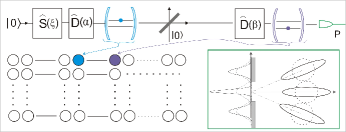
Figure 1: Entanglement distribution using squeezed-state ($|\alpha,\xi\rangle$) communication with reamplification ($\hat{D}(\beta)$). Reamplified phase-rotated squeezed states can be better discriminated through homodyne detection than unamplified coherent states.

Here we optimize Gaussian communication for the HQR scheme with the only restriction that the initial probe beam is in a pure state, and under the natural assumption that the initial squeezing direction and the final quadrature projection axis coincide. We will combine ingredients already exploited in Ref. PvL , i.e., dispersive atom-light interactions, a beam splitter loss model, and homodyne detection with squeezing and reamplification.

Ideal qubit-qumode interactions– For the initial entanglement distribution in an HQR, two neighboring stations are each equipped with a cavity containing a two-level system (qubit) and connected by a channel that can carry a quantized optical mode (qumode). The qumode is initially in a displaced squeezed vacuum state, $|\alpha,\xi\rangle=\hat{D}(\alpha)\hat{S}(\xi)|0\rangle$, with $\xi=re^{i\pi}$, real parameters $\alpha$ and $r$, and the displacement and squeezing operators $\hat{D}(\alpha)$ and $\hat{S}(\xi)$, respectively sq . The initial atomic states are each $(|0\rangle+|1\rangle)/\sqrt{2}$. Now a dispersive off-resonant interaction, $\hat{U}_{int}=\exp(i\theta\hat{n}\sigma_{z}/2)$, on the first qubit, where $\hat{n}$ is the photon number and $\sigma_{z}=|0\rangle\langle 0|-|1\rangle\langle 1|$ the Pauli $Z$ operator, leads to a conditional phase-rotation of the qumode, $\hat{U}_{int}\left[\frac{|0\rangle+|1\rangle}{\sqrt{2}}\otimes|\alpha,\xi\rangle\right]=\frac{|0\rangle\otimes|\alpha_{0},\xi_{0}\rangle+|1\rangle\otimes|\alpha_{1},\xi_{1}\rangle}{\sqrt{2}}$ with $\alpha_{k}=e^{\frac{i\theta(-1)^{k}}{2}}\alpha$, $\xi_{k}=e^{(-1)^{k}i\theta}\xi$, where $k=0,1$. After this first interaction, the qumode travels to the other cavity and interacts with the second qubit in a similar way. For a loss-free channel, the final qubit–qubit–qumode state is given by $\left[|0\rangle|0\rangle|e^{i\theta}\alpha,e^{2i\theta}\xi\rangle+|1\rangle|1\rangle|e^{-i\theta}\alpha,e^{-2i\theta}\xi\rangle\right.+\left.\big{(}|0\rangle|1\rangle+|1\rangle|0\rangle\big{)}|\alpha,\xi\rangle\right]/2$. By measuring the qumode in an appropriate way one can distinguish its initial state $|\alpha,\xi\rangle$ from the phase-rotated states and conditionally create an entangled state between the two cavities PvL .

Lossy channels– In the realistic scenario, two neighboring repeater stations are separated at least by a distance of $10-20$ km, linked by a lossy channel of this length. Thus, the qumode will be subject to attenuation and thermalization, especially when its initial state differs from a pure coherent state. In order to describe the resulting mixed-state density matrices, we define the operator $\hat{L}_{jk}$ [see Eq. (2) in Appendix “Methods”]; it characterizes our system after the interaction in the first cavity and the transmission through the lossy channel (derivation of $\hat{L}_{jk}$ and more details about the noise model can also be found in the Appendix).

While decoherence or thermalization are unavoidable in the lossy channel, the effect of attenuation may be corrected by an additional displacement operation $\hat{D}(\beta)$. Thus, before the interaction in the second cavity, we displace the light field by a suitably chosen, real $\beta$. The total state of the system (qumode and two qubits) after the second interaction is given by

$$\hat{\rho}\!=\!\!\!\displaystyle\sum_{l,m,j,k=0}^{1}\!\!\!|j,l\rangle\langle k,m|e^{\frac{i\theta\hat{n}}{2}(-1)^{l}}\hat{D}(\beta)\hat{L}_{jk}\hat{D}^{\dagger}(\beta)e^{\frac{i\theta\hat{n}}{2}(-1)^{m}}\!\!,$$ (1)

where the $l,m$ indices label the atomic states in the second cavity, while the indices $j,k$ refer to the first cavity. Now measuring the qumode subsystem of $\hat{\rho}$ leads to a conditional 4 by 4 two-qubit density matrix. In the case of homodyne detection of the $p$ quadrature,i.e., $\displaystyle{{\int_{-p_{c}}^{p_{c}}}}\!\langle p|\hat{\rho}|p\rangle\,dp$, we effectively select from $\hat{\rho}$ those terms corresponding to a mixture of $|\Psi^{\pm}\rangle=(|01\rangle\pm|10\rangle)/\sqrt{2}$ Bell states; the resulting phase-flip errors ($\pm$) stem from photon losses, minimal for small amplitudes $\alpha$; the finite overlaps of the Gaussian peaks in the homodyne-based approach lead to additional bit-flip errors, minimized for large amplitudes $\alpha$ PvL_3 . However, in our generalized scheme, we have as additional parameters the squeezing $r$ and the reamplification amplitude $\beta$, which have a significant impact on the above trade-off between channel decoherence and homodyne-based Gaussian-state distinguishability.

The final fidelity compared to the ideal Bell state $|\Psi^{+}\rangle$ now becomes $F=\displaystyle\int_{-p_{c}}^{p_{c}}\!\langle\Psi^{+}|\langle p|\hat{\rho}|p\rangle|\Psi^{+}\rangle\,dp/P_{s}\,.$ The normalization factor, $P_{s}=\mathrm{Tr}\left[\displaystyle\int_{-p_{c}}^{p_{c}}\!\langle p|\hat{\rho}|p\rangle\,dp\right]$, after tracing over the conditional qubit states, determines the probability of success, i.e., how frequently we actually obtain a measurement result within the postselection window $2p_{c}$. Exact expressions for $F$ and $P_{s}$ are given in the Appendix [Eqs. (3), (4)].

Results– Although the fidelity $F$ [Eq. (3)] is a highly oscillating function, we shall focus on its upper envelope $F_{Abs}$, calculated from $F$ by taking the absolute value instead of the real part of the last term in Eq. (3), as we may always “undo” the corresponding local phase (see Refs. PvL ; Ladd06 for details). From now on we assume fixed phase shift $\theta=0.01$ and transmission $T$, with losses corresponding to 0.17 dB/km. The fidelity then becomes a function of the squeezing parameter $r$, the initial amplitude $\alpha$, the displacement $\beta$, and the selection window $2p_{c}$. Varying $\alpha$, $\beta$, $r$ for every $p_{c}$, the maximum of $F_{Abs}$ can be found. The plots in Fig. 2 show the maximal $F_{Abs}$ with corresponding $P_{s}$ for different distances between repeater stations. We see that now near-unit fidelities can be achieved owing to squeezing and reamplification: for the selection window $p_{c}\rightarrow 0$, the maximal fidelities approach unity, at the expense of success probabilities tending to zero. This regime was previously accessible only through non-Gaussian measurements such as USD or in conceptually different single-photon-based schemes.

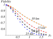
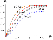
Figure 2: Fidelity $F_{Abs}$ and corresponding probability of success $P_{s}$ as a function of the selection window width $p_{c}$ for transmission distances 10, 15, 20, and 25 km, rotation angle $\theta=0.01$ and loss 0.17 dB/km. Free parameters used for optimization were: initial $\alpha$, squeezing parameter $r$, and displacement $\beta$.

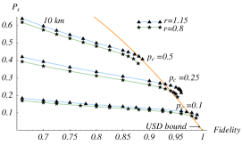
Figure 3: Maximal probability of success $P_{s}$ for given $F_{Abs}$ and different $p_{c}$ and $r$ (rotation angle is set to $\theta=0.01$, loss to 0.17 dB/km, and distance $L_{0}$ is 10 km). Maximal fidelity $F_{Abs}$ obtained choosing optimal initial $\alpha$ and displacement $\beta$ for $r=0.8$ and $r=1.15$ and $p_{c}=0.1$, $p_{c}=0.25$, $p_{c}=0.5$, respectively, is shown. Orange curve is the USD bound PvL_3 valid for coherent states.

Alternatively, we may obtain maximal $P_{s}$ for fixed F, $p_{c}$, and $r$, see Fig. 3 with $0.66\leq F_{Abs}\leq 1$, $L_{0}=10$ km, $p_{c}\in\{0.1,0.25,0.5\}$, and $r\in\{0.8,1.15\}$. For comparison we included the coherent-state USD bound PvL_3 (in orange), previously obtainable only through non-Gaussian POVMs jap2 . We observe that for sufficiently small selection windows, our scheme combining squeezed light, reamplification, and homodyne detection performs better then those based on single-photon detectors. Similar but slightly smaller improvements over the USD bound can be obtained for a distance of the order of the attenuation distance, $L_{0}=20$ km. A comparison of the standard HQR scheme PvL and ours with squeezing and reamplification is given in Fig. 4 and Table 1. The differences are significant. For $L_{0}=10$ km, both fidelities and probabilities of success are much higher in our scheme; for $L_{0}=20$ km, fidelities are highly increased, at the expense of smaller success probabilities.

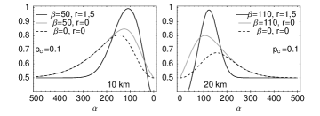
Figure 4: Fidelity $F_{Abs}$ as a function of initial $\alpha$. Dashed lines correspond to a coherent state as initial qumode state and no amplification, solid grey lines to a coherent state amplified, solid black lines to a squeezed state ($r=1.5$) amplified after transmission. Distance between cavities is $L_{0}=10$ or $20$ km, and amplification is just a displacement by $\hat{D}(\beta)$.

Table 1: Fidelities $F_{Abs}^{max}$ and probabilities of success $P_{s}$ corresponding to parameters from Fig. 4

initial state		squeezed,		coherent,		coherent, no
of light:		amplified		amplified		amplification
distance	$\;p_{c}\;$	$F_{Abs}^{max}$	$P_{s}$ [%]	$F_{Abs}^{max}$	$P_{s}$ [%]	$F_{Abs}^{max}$	$P_{s}$ [%]
10 km	$\;0.1\;$	0.99	9	0.85	7	0.80	8
	$\;0.25\;$	0.96	23	0.83	18	0.80	20
	$\;0.5\;$	0.89	40	0.80	33	0.77	36
20 km	$\;0.1\;$	0.98	4.5	0.79	5	0.68	9
	$\;0.25\;$	0.93	12	0.77	13	0.67	21
	$\;0.5\;$	0.81	26	0.71	26	0.63	39

Discussion– The results presented here are restricted to an elementary segment of a full HQR. Obviously, the present scheme gives a lot of freedom regarding optimal fidelity and probability of success, as a starting point for the subsequent procedures of entanglement swapping and purification. Even though in our generalized scheme, initial fidelities are high, we should stress that the resulting two-qubit entangled-state density matrices have non-zero elements for all four Bell states, as opposed to, for instance, the non-Gaussian USD-based scheme PvL_3 . The rank-2 mixtures there PvL_3 are typically easier to purify than the full rank-4 mixtures obtained from both photon-loss-induced phase-flip and measurement-induced bit-flip errors as in our scheme. We leave a full analysis, incorporating our scheme into a complete HQR including rank-4 purifications and swappings for future research. The reason why in our scheme we can suppress the loss-induced errors to a great extent is because we may keep the initial amplitudes $\alpha$ relatively small, but still have only small amounts of measurement-induced errors owing to squeezing and reamplification.

We note that different from existing proposals for distributing discrete entanglement through dynamical entanglement transfer from two-mode squeezed KrausCirac or general two-mode states Paternostro to discrete systems, our scheme makes explicit use of weak (dispersive, off-resonant) light-matter interactions and employs local measurements including postselection; photon losses are primarily assumed to occur in the channel as a limiting factor to the communication distance, instead of distance-independent dissipation during the local interactions KrausCirac ; Paternostro ; Chin .

Realistic qubit-qumode interactions– Finally, we address the question whether the idealized, controlled phase-rotation in our scheme can be indeed approximately realized; especially, when the qumode starts in a nonclassical, squeezed state. First of all, the effective Jaynes-Cummings-based interaction for the limiting case of large detuning in the off-resonant, dispersive regime holds for any input state of the qumode. However, in a cavity-QED setting, the internal cavity mode and the external fields are no longer identical; in particular, atomic spontaneous emissions (unwanted in-out couplings) and a finite desired cavity in-out coupling have to be taken into account. The master equation derived in Ref. Ladd06 under the Born approximation holds for any qumode state; in the relevant regime of $\alpha$ values, semi-classical calculations are sufficient, however, we have to assume that a squeezed state coupled into the cavity at least remains a Gaussian state at all times. As a result, non-Gaussian effects become negligible, similar to the case of coherent-state inputs of Ref. Ladd06 . The crucial parameter is then a sufficiently large cooperativity (“good coupling / dissipation”) at weak or intermediate coupling.

Squeezing may even turn out to be beneficial for the fidelity of the dispersive interaction Chin2 . In our model, coupling inefficiencies may be absorbed into the transmission parameter $T$, corresponding to reduced distances. Alternatively, the optical squeezing operation may be postponed until the very end, performed online Akira on phase-rotated coherent states. Besides CQED, approaches less sensitive to local dissipations may involve free-space light-matter couplings Savage ; Sondermann .

Acknowledgements– P.v.L. wants to thank Bill Munro and Kae Nemoto for their support when this research line was initiated. The authors acknowledge support from the Emmy Noether programme of the DFG in Germany.

I Methods

Beamsplitter noise model– we assume that the incident light mode $a$ interacts on a beamsplitter with an additional mode $b$ (initially in a vacuum state). After this interaction the trace over mode $b$ is taken, assuming no control over the loss mode. A beamsplitter transforms two incident modes according to the following unitary operation: $\hat{U}^{\dagger}_{\mathrm{B}}\hat{a}\hat{U}_{\mathrm{B}}=\hat{a}\sqrt{T}+i\,\hat{b}\sqrt{R}$, $\hat{U}_{\mathrm{B}}^{\dagger}\hat{b}\,\hat{U}_{\mathrm{B}}=\hat{b}\sqrt{T}+i\,\hat{a}\sqrt{R}$, where the standard relation between the reflection and transmission coefficients, i.e., $T+R=1$, holds. Thus, the interaction of a displaced squeezed vacuum state with a vacuum state on a beamsplitter leads to the following state:

$$|\psi_{ab}(\alpha,\xi)\rangle:=\hat{U}_{\mathrm{B}}\left[\big{(}\hat{D}(\alpha)\hat{S}(\xi)\otimes\mathds{1}\big{)}|0_{a};0_{b}\rangle\right]=$$

$$=\frac{1}{\sqrt{\mu}}\exp\left(\alpha\big{(}\sqrt{T}\hat{a}^{\dagger}+i\sqrt{R}\hat{b}^{\dagger}\big{)}-\alpha^{*}\big{(}\sqrt{T}\hat{a}-i\sqrt{R}\hat{b}\big{)}\right)$$

$$\exp\left[-\frac{\nu}{2\mu}\left(T\hat{a}^{\dagger 2}-R\hat{b}^{\dagger 2}+2i\sqrt{RT}\hat{a}^{\dagger}\hat{b}^{\dagger}\right)\right]|0_{a};0_{b}\rangle,$$

where $\mu=\cosh|\xi|$, $\nu=\xi/|\xi|\sinh|\xi|$.

Tracing over mode $b$, we find that the “light” part of an arbitrary element of the density matrix

$$\sum_{j,k=0}^{1}|j\rangle\langle k|\otimes|\alpha_{j},{\xi_{j}}\rangle\langle\alpha_{k},{\xi_{k}}|$$

that corresponds to

$$\hat{U}_{int}\left[\frac{|0\rangle+|1\rangle}{\sqrt{2}}\otimes|\alpha,\xi\rangle\right]=\frac{|0\rangle\otimes|\alpha_{0},\xi_{0}\rangle+|1\rangle\otimes|\alpha_{1},\xi_{1}\rangle}{\sqrt{2}}\,,$$

is transformed into:

$$L_{jk}:=\mathrm{Tr}_{b}\big{[}|\psi_{ab}(\alpha_{j},\xi_{j})\rangle\langle\psi_{ab}(\alpha_{k},\xi_{k})|\big{]}=e^{-\frac{|\alpha_{j}|^{2}+|\alpha_{k}|^{2}}{2}}e^{\alpha_{j}\alpha_{k}^{*}R}{\displaystyle{\iint}}\frac{\mathrm{d}^{2}\mathrm{H}}{\mu}\frac{\mathrm{d}^{2}\mathrm{J}}{\pi^{2}}e^{-|\mathrm{H}|^{2}-|\mathrm{J}|^{2}+\frac{\nu_{j}R}{2\mu}\mathrm{J}^{*2}+\frac{\nu_{k}^{*}R}{2\mu}\mathrm{H}^{2}+\mathrm{H}^{*}\mathrm{J}}\times$$

$$e^{i\sqrt{R}(\alpha_{j}^{*}-\alpha_{k}^{*})J}e^{\alpha_{j}\sqrt{T}\hat{a}^{\dagger}}e^{-\alpha_{j}^{*}\sqrt{T}\hat{a}}e^{-\frac{\nu_{j}T}{2\mu}\hat{a}^{\dagger 2}-i\frac{\nu_{j}\sqrt{RT}}{\mu}\hat{a}^{\dagger}\mathrm{J}^{*}}|0\rangle\langle 0|e^{i\frac{\nu_{k}^{*}\sqrt{TR}}{\mu}\hat{a}\mathrm{H}-\frac{\nu_{k}^{*}T}{2\mu}\hat{a}^{2}}e^{-\alpha_{k}\sqrt{T}\hat{a}^{\dagger}}e^{\alpha_{k}^{*}\sqrt{T}\hat{a}}e^{i\sqrt{R}(\alpha_{j}-\alpha_{k})\mathrm{H}^{*}}$$ (2)

where ${\mathrm{d}}^{2}\mathrm{H}={\mathrm{d}}(\mathrm{Re}\mathrm{H})\mathrm{d}(\mathrm{Im}\mathrm{H})$, ${\mathrm{d}}^{2}\mathrm{J}={\mathrm{d}}(\mathrm{Re}\mathrm{J})\mathrm{d}(\mathrm{Im}\mathrm{J}$).

Fidelity, Probability of success– After the transmission through a lossy channel the light is reamplified by applying a displacement operator $\hat{D}(\beta)$ to the qumode. Then the qumode interacts with the atom in the second cavity, and is finally detected by a homodyne measurement of the $p$-quadrature. In our notation, we have $\hat{x}=(\hat{a}+\hat{a}^{\dagger})/2$, $\hat{p}=(\hat{a}-\hat{a}^{\dagger})/(2i)$; corresponding to a commutator $[\hat{x},\hat{p}]=i/2$. The total state of the system before measurement is described by $\hat{\rho}$ from Eq. (1). The fidelity of the (renormalized) conditional state measured within the postselection window [-$p_{c}$, $p_{c}$], compared to the ideal Bell state $|\Psi^{+}\rangle$, reads as follows:

$$F=\frac{1}{P_{s}}\displaystyle\int_{-p_{c}}^{p_{c}}\!\langle\Psi^{+}|\langle p|\hat{\rho}|p\rangle|\Psi^{+}\rangle\,dp=\frac{1}{P_{s}}\left\{\mathrm{Erf}\left[\frac{\sqrt{2}(p_{c}-\beta\sin\frac{\theta}{2})}{\sqrt{1+2T\nu(\nu+\mu)}}\right]+\mathrm{Erf}\left[\frac{\sqrt{2}(p_{c}+\beta\sin\frac{\theta}{2})}{\sqrt{1+2T\nu(\nu+\mu)}}\right]+\right.$$ (3)

$$2\mathrm{Re}\left\{\frac{\mathrm{Erf}\left[p_{c}\sqrt{\frac{2(\mu-\nu(T+e^{i\theta}R))}{\mu+\nu(T-e^{i\theta}R)}}\right]}{\sqrt{\mu^{2}-\nu^{2}(T+e^{{i\theta}}R)^{2}}}\right.\left.\left.\exp\left[\frac{2i\alpha\sin\frac{\theta}{2}\left(\alpha e^{\frac{i\theta}{2}}R-2\beta\sqrt{T}\right)}{\mu+\nu(T+e^{i\theta}R)}-\frac{2i\beta^{2}\sin\frac{\theta}{2}\left(\mu^{2}e^{-\frac{i\theta}{2}}-\nu^{2}\left(e^{\frac{i\theta}{2}}T+e^{\frac{3i\theta}{2}}R\right)+i\mu\nu T\sin\frac{\theta}{2}\right)}{\mu^{2}-\nu^{2}(T+e^{{i\theta}}R)^{2}}\right]\right\}\right\}.$$

Squeezing enters the above formula through $\mu=\cosh r$ and $\nu=-\sinh r$, characterizing, together with $\alpha$, the initial qumode state. The parameter $\theta$ determines the atom-light interaction, loss is introduced through $T$ and $R=1-T$, i.e., the beamsplitter transmission/reflection coefficients, and $\beta$ describes the (re-)amplification via the displacement operator. The corresponding probability of success is given by:

$$P_{s}=\frac{1}{4}\big{[}\mathrm{Erf}(c_{00})+\mathrm{Erf}(c_{01})+\mathrm{Erf}(c_{10})+\mathrm{Erf}(c_{11})\big{]}, \mathrm{where} c_{nm}=\frac{\sqrt{2}\left\{p_{c}-(-1)^{n}\left[\beta\sin\frac{\theta}{2}+\sqrt{T}\alpha\sin(m\theta)\right]\right\}}{\sqrt{1+2T\nu(\nu+\mu\cos(2m\theta))}}\,,$$ (4)

and $n,m=0,1$.

References

- (1) D. Stucki et al., New J. Phys. 11, 075003 (2009).
- (2) N. Gisin et al., Rev. Mod. Phys. 74, 145 (2002).
- (3) T. Scheidl et al., New J. Phys. 11, 085002 (2009).
- (4) H.-J. Briegel et al., Phys. Rev. Lett. 81, 5932 (1998)
- (5) W. Dür et al., Phys. Rev. A 59, 169 (1999).
- (6) N. Sangouard et al., quant-ph:0906.2699 (2009).
- (7) C. H. Bennett et al., Phys. Rev. Lett. 76, 722 (1996); C. H. Bennett et al., Phys. Rev. A 54, 3824 (1996).
- (8) D. Deutsch et al., Phys. Rev. Lett. 77, 2818 (1996).
- (9) L. Hartmann et al., Phys. Rev. A 75, 032310 (2007).
- (10) L. M. Duan et al., Nature 414, 413 (2001).
- (11) L. Childress et al., Phys. Rev. A 72, 052330 (2005); Phys. Rev. Lett. 96, 070504 (2006).
- (12) P. van Loock et al., Phys. Rev. Lett. 96, 240501 (2006).
- (13) L. Jiang et al., PNAS 104, 17291 (2007).
- (14) W. J. Munro et al., Phys. Rev. Lett. 101, 040502 (2008).
- (15) P. van Loock et al., Phys. Rev. A 78, 062319 (2008).
- (16) K. Azuma et al., quant-ph: 0811.3100
- (17) S. M. Barnett, P. M. Radmore, Methods in Theoretical Quantum Optics, Oxford series in optical and imagining science; 15.
- (18) B. Kraus et al.,Phys. Rev. Lett. 92, 013602 (2004).
- (19) M. Paternostro et al.,Phys. Rev. Lett. 92, 197901 (2004).
- (20) F.Yu Hong et al., J. of Mod. Opt., 55, 2731-2737 (2008).
- (21) T. D. Ladd et al., New J. Phys. 8, 184 (2006).
- (22) F.Yu Hong et al.,Eur. Phys. J. D 54, 131 (2009).
- (23) Y. Miwa et al., Phys. Rev. A 80, 050303(R) (2009).
- (24) C. M. Savage et al., Opt. Lett. 15, 628 (1990).
- (25) M. Sondermann et al., Appl. Phys. B 89, 489 (2007).