Characterizing the linear growth rate of cosmological density perturbations in an $f(R)$ model

Abstract

We investigate the linear growth rate of cosmological matter density perturbations in a viable $f(R)$ model both numerically and analytically. We find that the growth rate in the scalar-tensor regime can be characterized by a simple analytic formula. We also investigate a prospect of constraining the Compton wavelength scale of the $f(R)$ model with a future weak lensing survey.

I Introduction

Cosmological observations of distant Ia supernovae discovered that our Universe is undergoing an accelerated expansion period Riess98 ; Perlmutter99 , which is supported by other observations of the cosmic microwave background anisotropies and the large scale structure of galaxies WMAP3 ; Einsenstein05 ; Percival07 . These observations are explained by the cosmological model with the cosmological constant $\Lambda$. The cosmological constant can be regarded as the vacuum energy, however, the smallness of the observed value raises a fine-tuning problem Weinberg . To explain the cosmic accelerated expansion, many dark energy models have been proposed (see e.g., Peebles ; DE06 and the references therein). Modification of the gravity theory is an alternative approach, for example, $f(R)$ model Carroll ; Nojiri ; Capozziello ; Sotiriou08 and the Dvali, Gabadadze, and Porrati (DGP) model in the context of the braneworld scenario DGP .

Many authors have studied dynamical dark energy models Huterer01 ; Chevallier ; Linder03 ; Sahni08 . Dynamical dark energy models may have similar expansion rates to models of modified gravity, because modification of the gravity theory may affect the background expansion history. Therefore, the observations of the background expansion history alone are unable to distinguish between modified gravity and dynamical dark energy. The key to distinguish between modified gravity and dynamical dark energy is the growth of cosmological perturbations Ishak06 ; Yamamoto07 ; Huterer07 ; Kunz07 ; Song09 ; Koyama09 . The growth history of cosmological perturbations can be tested with the large scale structure in the Universe. Many projects of large survey of galaxies are in progress or planned DETF06 ; Frieman08 ; sdss3 ; sumire ; lsst ; ska ; Robberto ; DES ; Pan-STARRS ; Euclid , and these surveys might give us a hint in exploring the origin of the accelerated expansion of the Universe and the nature of gravity LinderRD ; Nesseris08 ; Porto08 ; Heavens07 ; Zhang07 ; Amendola08 ; Schmidt08 ; Song08 ; Tsujikawa08a ; Thomas09 ; Zhao09a ; Zhao09b ; Guzik09 ; Bean09 .

Cosmological perturbations in modified gravity models have been investigated by many authors Linder05 ; Knox06 ; Linder07 ; Gong08 ; Sereno06 ; Wang08 ; Polarski08 ; Ballesteros08 ; Gannouji08a ; Gannouji08b ; Bertschinger08 ; Laszlo08 ; Wei08 ; Dent09a ; Dent09b . In the present paper, we investigate the growth history of matter density perturbations in $f(R)$ models. $f(R)$ model is a modified gravity model, constructed by replacing the gravitational Lagrangian with a general function of the Ricci scalar $R$. The viable $f(R)$ models have been proposed Starobinsky07 ; HuSawicki07 ; Battye ; Tsujikawa08 ; Tsujikawa09 , which explain the late-time accelerate expansion of the background Universe, and satisfy the local gravity constraints. The viable model which also explains an inflationary epoch in the early Universe is extensively proposed Nojiri07a ; Nojiri07b ; Cognola . For the local gravity constraints, the chameleon mechanism is supposed to play an important role Mota04 ; Khoury04 ; Brax08 . By this mechanism, a field that modifies the gravity is hidden in the local region with high density. We note that a problem of the theory in the strong gravity regime is under debate Kobayashi ; Upadye . Though the evolution of cosmological perturbations in $f(R)$ models has been studied so far Pogosian ; Song07 ; Bean07 ; Tsujikawa07 ; delaCD ; Motohashi ; Brax09 ; Zhang06 ; Capozziello09 ; Carloni09 , our investigation is focused on a new description of the growth rate for the $f(R)$ model.

This paper is organized as follows. In Sec. II, we briefly review the viable $f(R)$ models. In Sec. III, we investigate the evolution of density perturbations in the $f(R)$ model both numerically and analytically. We find that the growth rate of density perturbations can be characterized by a simple analytic formula, which approximately describes the growth rate in the scalar-tensor regime. The growth rate in the general-relativity regime is also investigated. In Sec. IV, we investigate a future prospect of constraining the $f(R)$ model assuming a future large survey of weak lensing statistics on the basis of the Fisher matrix analysis. Section V is devoted to summary and conclusions. Throughout the paper, we use the unit in which the speed of light equals 1 and $\hbar=1$.

II a brief review of $f(R)$ model

We briefly review $f(R)$ model, which is defined by the action,

$$S=\frac{1}{16\pi G}\int d^{4}x\sqrt{-g}(R+f(R))+\int d^{4}x\sqrt{-g}L^{(\rm m)},$$ (1)

where $G$ is the gravitational constant, and $L^{(\rm m)}$ is the matter Lagrangian density. We consider the viable models, proposed in Refs.  Starobinsky07 ; HuSawicki07 ; Battye ; Tsujikawa08 ; Tsujikawa09 . The viable models have an asymptotic formula at the late-time Universe ($R\gg R_{c}$), which can be written as

$$f(R)=-\lambda R_{c}\left[1-\left({R_{c}\over R}\right)^{2n}\right],$$ (2)

where $R_{c}$ is a positive constant whose value is the same order as that of the present Ricci scalar, and $\lambda$ is a nondimensional constant. Because the term $\lambda R_{c}$ plays a role of the cosmological constant, we may write $\lambda R_{c}=6(1-\Omega_{0})H_{0}^{2}$, where $H_{0}$ is the Hubble constant and $\Omega_{0}$ is the matter density parameter. Note that we assume the spatially flat Universe.

It is well known that $f_{R}=df(R)/dR$ plays a roll of a new degree of freedom, which behaves like a scalar field with the mass

$$m^{2}={1\over 3}\left({1+f_{R}\over f_{RR}}-R\right),$$ (3)

where we defined $f_{RR}={d^{2}f(R)/dR^{2}}$. Assuming $|f_{R}|\ll 1$ and $Rf_{RR}\ll 1$ for the viable model, the mass is simply $m^{2}=1/(3f_{RR})$.

We focus on the evolution of matter density perturbations in the $f(R)$ model, whose Fourier coefficients obey (e.g., Tsujikawa09 )

$$\ddot{\delta}+2H\dot{\delta}-4\pi G_{\rm eff}\rho\delta=0,$$ (4)

where the dot denotes the differentiation with respect to the cosmic time, $H=\dot{a}/a$ is the Hubble parameter, $\rho$ is the matter mean density, and $G_{\rm eff}$ is the effective gravitational constant, which is written as

$${G_{\rm eff}\over G}=1+{1\over 3}{k^{2}/a^{2}\over k^{2}/a^{2}+1/(3f_{RR})},$$ (5)

where $k$ is the wave number, and $a$ is the scale factor normalized to unity at present epoch (cf. Zhang06 ). As is noted in the above, the physical meaning of $m^{2}=1/(3f_{RR})$ is the square of the mass of the new degree of freedom which modifies the gravity force. We have the general-relativity regime, $G_{\rm eff}=G$, for $k/a\ll m$, and the scalar-tensor regime, $G_{\rm eff}=4G/3$, for $k/a\gg m$, respectively. Thus, the evolution of matter density perturbations depends on the wavenumber $k$, whose behavior is determined by the mass $m^{2}=1/(3f_{RR})$.

For the Einstein de Sitter universe, the exact solution of Eq. (4) is found in the literature Motohashi . However, we consider the low density universe, where the solution of Eq. (4) is described in a different form in comparison with that of Motohashi . From Eq. (2), we have

$$f_{RR}={d^{2}f(R)\over dR^{2}}=2n(2n+1)\lambda R_{c}{R_{c}^{2n}\over R^{2n+2}}.$$ (6)

Furthermore, using the formulas $\lambda R_{c}=6(1-\Omega_{0})H_{0}^{2}$ and $R=3H_{0}^{2}\left[{\Omega_{0}/a^{3}}+4(1-\Omega_{0})\right]$, we have

$${1\over 3f_{RR}}={\Omega_{0}H_{0}^{2}\over 4n(2n+1)}\left({\lambda\over 2}\right)^{2n}\left({\Omega_{0}\over 1-\Omega_{0}}\right)^{2n+1}\left({1\over a^{3}}+{4(1-\Omega_{0})\over\Omega_{0}}\right)^{2n+2}.$$ (7)

Denoting the wavenumber corresponding to the Compton wavelength $1/m$ at the present epoch by $k_{C}$,

$$k_{C}^{2}={\Omega_{0}H_{0}^{2}\over 4n(2n+1)}\left({\lambda\over 2}\right)^{2n}\left({\Omega_{0}\over 1-\Omega_{0}}\right)^{2n+1}\left({1}+{4(1-\Omega_{0})\over\Omega_{0}}\right)^{2n+2},$$ (8)

Equation (7) is rewritten as

$${1\over 3f_{RR}}=k_{C}^{2}\left({\Omega_{0}{a^{-3}}+{4(1-\Omega_{0})}\over{\Omega_{0}}+{4(1-\Omega_{0})}}\right)^{2n+2}.$$ (9)

We denote the growth factor by $D_{1}(a,k)$, which is the solution of Eq. (4) normalized so as to be $D_{1}(a,k)\simeq a$ at $a\ll 1$. The growth rate is defined by

$$f(a,k)={d\log D_{1}(a,k)\over d\log a}.$$ (10)

Using the growth rate $f(a,k)$, Eq. (4) is rephrased as

$${df\over d\ln a}+f^{2}+\left(2+{\dot{H}\over H^{2}}\right)f={3\over 2}{G_{\rm eff}\over G}\Omega_{m}(a),$$ (11)

where $\Omega_{m}(a)$ is defined by $\Omega_{m}(a)={H_{0}^{2}\Omega_{0}a^{-3}/H^{2}}$. We assume that the background expansion is well approximated by the $\Lambda$CDM model, where the Hubble parameter satisfies

$${\dot{H}\over H^{2}}=-{3\over 2}\Omega_{m}(a),$$ (12)

and the energy conservation equation

$${d\Omega_{m}(a)\over d\ln a}=-3\Omega_{m}(a)(1-\Omega_{m}(a)).$$ (13)

Using Eqs. (11)-(13) yields

$$-3\Omega_{m}(a)(1-\Omega_{m}(a)){df\over d\Omega_{m}(a)}+f^{2}+\left(2-{3\over 2}\Omega_{m}(a)\right)f={3\over 2}{G_{\rm eff}\over G}\Omega_{m}(a),$$ (14)

which is useful to find an approximate solution, as we see in the next section.

III growth of density perturbations in $f(R)$ model

In this section, we investigate the evolution of matter density perturbations in the $f(R)$ model. In Sec. III A, we consider the scalar-tensor regime, $k/a\gg m$, in which the wavelength is shorter than the Compton wavelength. In Sec. III B, we consider the general-relativity regime, $k/a\ll m$, in which the wavelength is larger than the Compton wavelength.

III.1 scalar-tensor regime

In the scalar-tensor regime, $k/a\gg m$, the effective gravitational constant becomes $G_{\rm eff}=4G/3$. In this case, we find that Eq. (14) has the solution expressed in the form footnote1

$$f(a,k)=f_{0}\Omega_{m}(a)^{\widetilde{\gamma}(a)},$$ (15)

where $f_{0}$ obeys $f_{0}^{2}+f_{0}/2=2$, therefore $f_{0}=(-1+\sqrt{33})/4$, and

$$\widetilde{\gamma}(a)=\sum_{\ell=0}\zeta_{\ell}(1-\Omega_{m}(a))^{\ell},$$ (16)

where $\zeta_{\ell}$ is the expansion coefficients. The first few terms of $\widetilde{\gamma}(a)$ are

$$\widetilde{\gamma}(a)={9-\sqrt{33}\over 6}-{93-17\sqrt{33}\over 666}\left(1-\Omega_{m}(a)\right)+{\cal O}\left((1-\Omega_{m}(a))^{2}\right).$$ (17)

This can be generalized to the case when $G_{\rm eff}/G(={\xi})$ is a constant value, in which the solution of Eq. (11) has the same formula as that of (15) but with $f_{0}=({-1+\sqrt{1+24{\xi}}})/{4}$ and

$${\widetilde{\gamma}}(a)=\frac{-41+24{\xi}+\sqrt{1+24{\xi}}}{-70+48{\xi}}+{1\over 8(-143+24{\xi})(-35+24{\xi})^{2}}$$

$$~{}~{}~{}~{}~{}~{}\times\Bigl{[}(-41+24{\xi}+\sqrt{1+24{\xi}})\bigl{(}347-17\sqrt{1+24{\xi}}+24{\xi}(-13+\sqrt{1+24{\xi}})\bigr{)}\Bigr{]}$$

$$~{}~{}~{}~{}~{}~{}\times(1-\Omega_{m}(a))+{\cal O}\left((1-\Omega_{m}(a))^{2}\right).$$ (18)

Here we assume that $G_{\rm eff}/G(={\xi})$ is constant, but we utilize this formula by replacing ${\xi}$ with the right-hand-side of Eq. (5).

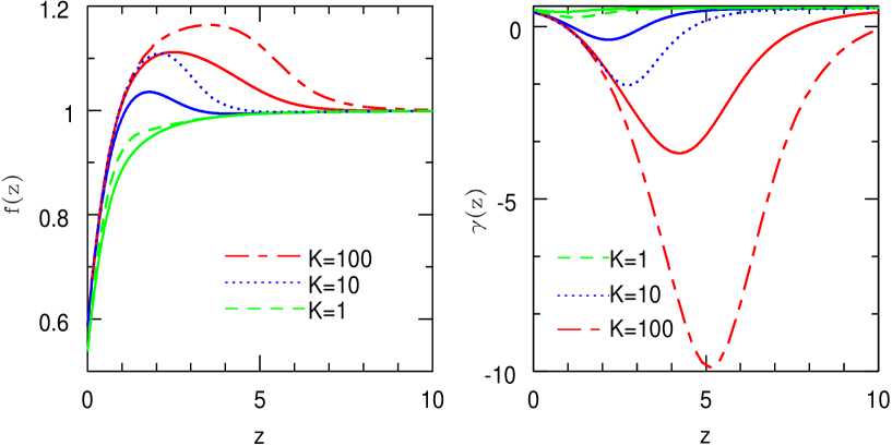
Figure 1: Left panel: $f(a,k)$ as a function of $z(=1/a-1)$ for the model $n=1$. The solid curves are obtained by solving the differential equation (11) numerically, for $K(=k/k_{C})=10^{2}$, $10$, and $1$, respectively, from the top to the bottom. The long dashed curve, the dotted curve and the short dashed curve adopt the approximate formula, for $K(=k/k_{C})=10^{2}$, $10$, and $1$, respectively, from the top to the bottom. Right panel: The growth index $\gamma(a,k)$ as a function of $z(=1/a-1)$, corresponding to the left panel. The parameter of the curves is the same as that of the left panel. The curves correspond to $K(=k/k_{C})=10^{2}$ and $10$, $1$ respectively, from the bottom to the top.

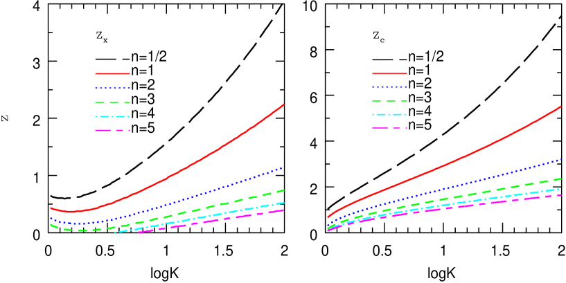
Figure 2: Left panel: Redshift $z_{x}$ when the difference of the growth rate becomes $f^{(\rm appr)}-f^{(\rm exac)}=0.03$, as a function of $K(=k/k_{C})$. The curves are $n=1/2,~{}1,~{}2,~{}3,~{}4$, and $5$, respectively, from the top to the bottom. Right panel: Transition redshift $z_{c}$ as a function of $K(=k/k_{C})$. From the top to the bottom, curves are $n=1/2,~{}1,~{}2,~{}3,~{}4$, and $5$, respectively. Here we adopted the background expansion of the Universe is the $\Lambda$CDM model with $\Omega_{0}=0.28$.

The left panel of Fig. 1 shows the growth rate $f(a,k)$ as a function of the redshift $z(=1/a-1)$. Here we adopted $n=1$. The solid curves are obtained by solving Eq. (11) numerically, for $K(=k/k_{C})=10^{2},~{}10,~{}1$, from the top to the bottom, respectively. Here we assumed the background expansion of the Universe is the $\Lambda$CDM model with $\Omega_{0}=0.28$. The dot-dashed curve, the dotted curve, and the short dashed curve are the approximate formula up to 1st order of $(1-\Omega_{m}(a))$, for the wavenumber $K(=k/k_{C})=10^{2},~{}10,~{}1$, respectively. In the computation of the approximate formula, we adopted the right-hand-side of Eq. (5) as $\xi$. One can see that the approximate solution approaches the exact solution at the late time of the redshift.

Following the previous works (e.g., see Polarski08 ), the growth index $\gamma(a,k)$ is introduced by

$$f(a,k)=\Omega_{m}(a)^{\gamma(a,k)},$$ (19)

which is related with $\widetilde{\gamma}(a,k)$ by

$${\gamma(a,k)={\ln f_{0}\over\ln\Omega_{m}(a)}+\widetilde{\gamma}(a,k)}.$$ (20)

The behavior of the growth index $\gamma(a,k)$ in the scalar-tensor regime is well approximated by Eq. (20), as is demonstrated in the right panel of Fig. 1, which plots $\gamma(a,k)$ as a function of the redshift $z$, for the wavenumber $K(=k/k_{C})=10^{2},~{}10,~{}1$, from the bottom to the top, respectively. The solid curves are obtained by solving Eqs. (11) and (19) numerically, for $K(=k/k_{C})=10^{2},~{}10,~{}1$, from the bottom to the top, respectively. The dot-dashed curve, the dotted curve, and the short dashed curve are the approximate solution of $\widetilde{\gamma}(a,k)$ and (20), for $K(=k/k_{C})=10^{2},~{}10,~{}1$, respectively. One can see that the approximate solution approaches the exact solution at the late time of the redshift, however, the validity is limited to the late time of the small redshift.

Let us discuss the valid region of the approximate solution. The left panel of Fig. 2 plots the redshift $z_{x}$ as a function of $K(=k/k_{C})$ for $n=1/2,~{}1,~{}2,~{}3,~{}4$, and $5$, respectively, from the top to the bottom, where $z_{x}$ is defined by the redshift when the difference of the growth rate becomes $f^{(\rm appr)}-f^{(\rm exac)}=0.03$. Here $f^{(\rm exac)}$ is the exact solution obtained by solving Eq. (11) numerically, while $f^{(\rm appr)}$ is the approximate solution. Thus, the approximate solution of the growth rate approaches the exact solution after the redshift $z_{x}$, which depends on $k/k_{C}$ as well as $n$. As $n$ is larger or $k/k_{C}$ is smaller, $z_{x}$ becomes smaller. For the case $n\geq 4$ and smaller value of $k/k_{C}$, we have no solution of $z_{x}$.

The above behavior is related with the transition redshift $z_{c}$, when the scalar-tensor regime starts, which we defined by $k(1+z_{c})=m$, i.e.,

$${k^{2}(1+z_{c})^{2}}=k_{C}^{2}\left({{\Omega_{0}(1+z_{c})^{3}}+{4(1-\Omega_{0})}\over{\Omega_{0}}+{4(1-\Omega_{0})}}\right)^{2n+2}.$$ (21)

The right panel of Fig. 2 plots $z_{c}$ as function of $K(=k/k_{C})$ for $n=1/2,~{}1,~{}2,~{}3,~{}4,~{}5$, respectively, from the top to the bottom. Figure 2 shows $z_{x}<z_{c}$. Thus the approximate formula approaches the exact solution after the scalar-tensor regime starts. For the model with larger value of $n$, the Compton scale evolves rapidly. Then, the transition redshift $z_{c}$ becomes small as $n$ becomes large. For the smaller value of $K(=k/k_{C})$, the transition redshift $z_{c}$ becomes smaller. This is the reason why $z_{x}$ is smaller, as $n$ is larger or $k/k_{C}$ is smaller. Therefore, for the case when $n$ is large and $k/k_{C}$ is smaller, the redshift when the approximate formula starts to work becomes later. For the case $n\lower 2.15277pt\hbox{$\;\buildrel<\over{\sim}\;$}2$, the late-time behavior of the growth rate can be approximated by the approximate formula as long as $K\lower 2.15277pt\hbox{$\;\buildrel>\over{\sim}\;$}1$.

We here mention the relation between the parameter $k_{C}$ and the parameter $f_{R0}$ adopted in Refs.  HuSawicki07 ; Schmidt09 , in which the case $n=1/2$ is investigated. In this case, $|f_{R0}|=2(1-3\Omega_{0}/4)H_{0}^{2}/k_{C}^{2}$. For $|f_{R0}|\simeq 10^{-4}-10^{-6}$, we have $k_{C}\simeq 0.04-0.4~{}h{\rm Mpc}^{-1}$. The scalar-tensor regime appears rather earlier in this model, as shown in Fig. 2.

III.2 general-relativity regime

In this subsection, we consider the growth rate of density perturbations at the early time epoch of the Universe, $a\ll 1$, adopting the approximation,

$${1\over 3f_{RR}}={\Omega_{0}H_{0}^{2}\over 4n(2n+1)}\left({\lambda\over 2}\right)^{2n}\left({\Omega_{0}\over 1-\Omega_{0}}\right)^{2n+1}\left({1\over a}\right)^{6n+6},$$ (22)

which yields the simple form of the effective gravitational constant

$${G_{\rm eff}\over G}=1+{1\over 3}{k^{2}\over k^{2}+k_{0}^{2}a^{-3N}},$$ (23)

where

$$N=2n+{4\over 3},$$ (24)

$$k_{0}^{2}={\Omega_{0}H_{0}^{2}\over 4n(2n+1)}\left({\lambda\over 2}\right)^{2n}\left({\Omega_{0}\over 1-\Omega_{0}}\right)^{2n+1}.$$ (25)

As mentioned in the previous section, $3f_{RR}$ has the meaning of the square of the Compton wavelength. Thus this model can be regarded as the model that the Compton wavelength simply evolves as $1/m=a^{3N/2+1}/k_{0}$.

In the case when $N$ is a positive integer, we derive an approximate solution of Eq. (11) in an analytic manner. With the use of (19), one can rewrite Eq. (14) as

$$-3\Omega_{m}(a)(1-\Omega_{m}(a))\ln\Omega_{m}(a)\frac{d\gamma}{d\Omega_{m}(a)}+3\Omega_{m}(a)\left(\gamma-\frac{1}{2}\right)+\Omega_{m}(a)^{\gamma}-\frac{3}{2}\frac{G_{\rm eff}}{G}\Omega_{m}(a)^{1-\gamma}-3\gamma+2=0.$$ (26)

In a straightforward manner, we find the solution for $\gamma(a,k)$ expanded in terms of $1-\Omega_{m}(a)$, as follows.

$$\gamma(a,k)=\sum_{\ell=0}\zeta_{\ell}(a,k)(1-\Omega_{m}(a))^{\ell},$$ (27)

where $\zeta_{\ell}(a,k)$ is the expansion coefficient. For example, for $N=1$, we find

$$\displaystyle{\gamma(a,k)={6\over 11}-\frac{K^{2}\Omega_{0}}{11(1-\Omega_{0})}}$$

$$\hskip 34.14322pt\displaystyle{+\left[\frac{15}{2057}-\frac{131K^{2}\Omega_{0}}{4114(1-\Omega_{0})}+\frac{263K^{4}\Omega_{0}^{2}}{4114(1-\Omega_{0})^{2}}\right](1-\Omega_{m}(a))+{\cal O}\left((1-\Omega_{m}(a))^{2}\right)},$$ (28)

where $K=k/k_{0}$. We also have

$$\gamma(a,k)=\displaystyle{\frac{6}{11}+\left[\frac{15}{2057}-\frac{K^{2}\Omega_{0}^{2}}{17(1-\Omega_{0})^{2}}\right](1-\Omega_{m}(a))}~{}~{}~{}~{}~{}~{}~{}~{}~{}~{}~{}~{}~{}~{}~{}~{}~{}~{}~{}~{}~{}~{}~{}~{}~{}~{}~{}~{}~{}~{}~{}~{}$$

$$\hskip 34.14322pt\displaystyle{+\left[\frac{4205}{1040842}-\frac{643K^{2}\Omega_{0}^{2}}{8602(1-\Omega_{0})^{2}}\right](1-\Omega_{m}(a))^{2}+{\cal O}\left((1-\Omega_{m}(a))^{3}\right),}$$ (29)

for $N=2$,

$$\gamma(a,k)=\displaystyle{\frac{6}{11}+\frac{15}{2057}(1-\Omega_{m}(a))}~{}~{}~{}~{}~{}~{}~{}~{}~{}~{}~{}~{}~{}~{}~{}~{}~{}~{}~{}~{}~{}~{}~{}~{}~{}~{}~{}~{}~{}~{}~{}~{}~{}~{}~{}~{}~{}~{}~{}~{}~{}~{}~{}~{}~{}~{}~{}~{}~{}~{}~{}~{}~{}~{}~{}~{}~{}~{}~{}$$

$$\hskip 34.14322pt\displaystyle{+\left[\frac{4205}{1040842}-\frac{K^{2}\Omega_{0}^{3}}{23(1-\Omega_{0})^{3}}\right](1-\Omega_{m}(a))^{2}+{\cal O}\left((1-\Omega_{m}(a))^{3}\right)},~{}~{}~{}$$ (30)

for $N=3$,

$$\gamma(a,k)=\displaystyle{\frac{6}{11}+\frac{15}{2057}(1-\Omega_{m}(a))+\frac{4205}{1040842}(1-\Omega_{m}(a))^{2}}~{}~{}~{}~{}~{}~{}~{}~{}~{}~{}~{}~{}~{}~{}~{}~{}~{}~{}~{}~{}~{}~{}~{}~{}~{}~{}~{}~{}~{}$$

$$\hskip 34.14322pt\displaystyle{+\left[\frac{31449595}{11288972332}-\frac{K^{2}\Omega_{0}^{4}}{29(1-\Omega_{0})^{4}}\right](1-\Omega_{m}(a))^{3}+{\cal O}\left((1-\Omega_{m}(a))^{4}\right)},$$ (31)

for $N=4$, respectively.

Figure 3 demonstrates the validity of the approximate formulas, by plotting the relative difference between the exact solution $f$ and the approximate solution $\Omega_{m}^{\gamma}$ as a function of the redshift. The four panels assume $N=1,~{}2,~{}3,~{}4$, respectively. In each panel, the cases of the wavenumber $K(=k/k_{C})=1,~{}0.1,~{}0.01$, are plotted. The solid curve, the dotted curve and the dashed curve correspond to $K=1,~{}0.1,~{}0.01$, respectively. For $N=1$, we used the approximate formula (28) up to the $1$st order of $(1-\Omega_{m}(a))$. For $N=2$, we used the approximate formula (29) up to the $2$nd order of $(1-\Omega_{m}(a))$. For $N=3$, we used the approximate formula (30) up to the $2$nd order of $(1-\Omega_{m}(a))$. For $N=4$, we used the approximate formula (31) up to the $3$rd order of $(1-\Omega_{m}(a))$. Even if we adopted higher order term of (28)$\sim$(31), the approximate formula only slightly improves the accuracy for $K=1$. The approximate formula is valid for $K\lower 2.15277pt\hbox{$\;\buildrel<\over{\sim}\;$}0.1$.

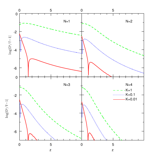
Figure 3: The relative difference of the growth factor between the exact solution $f$, which is obtained by solving Eq. (11) numerically, and the approximate solution in the form $\Omega_{m}^{\gamma}$, as a function of $z$. The four panels correspond to $N=1,~{}2,~{}3,$ and $4$, respectively. In each panel, the curves correspond to $K=0.01$, $0.1$, $1$, respectively, from the bottom to the top.

IV Constraint on $f(R)$ model from weak lensing survey

Cosmological constraints on the $f(R)$ model have been investigated in Refs. HuSawicki07 ; Schmidt09 ; Girones ; Yamamoto10 . The weak lensing statistics is useful to obtain a constraint on the growth history of cosmological density perturbations observationally. We now consider a prospect of constraining the $f(R)$ model with a future large survey of the weak lensing. To this end, we adopt the Fisher matrix analysis, which is frequently used for estimating minimal attainable constraint on the model parameters. To be self-contained, we summarized the fisher matrix analysis in the Appendix (see also Yamamoto07 , and the references therein). Here we focus on the constraint on the Compton wavenumber parameter $k_{C}$ defined by Eq. (8) or (9). In this analysis, we obtained the growth rate and the growth factor by numerically solving Eq. (11) and

$$D_{1}(a,k)=a\exp\left[\int_{0}^{a}{da^{\prime}\over a^{\prime}}(f(a^{\prime},k)-1)\right],$$ (32)

without using the approximate formula.

We briefly review how the signal of the weak lensing reflects the modification of the gravity in the $f(R)$ model. In the Newtonian gauge, the metric perturbations of the Universe can be describe by the curvature perturbation $\Phi$ and the potential perturbation $\Psi$,

$$ds^{2}=-\left(1+2\Psi\right)dt^{2}+a^{2}(t)\left(1+2\Phi\right)d{\bf x}^{2}.$$ (33)

In the $f(R)$ model, the relations between the two metric potentials and the matter density perturbations are altered. In the subhorizon limit, the $f(R)$ model yields (e.g., Silvestri and references therein)

$$k^{2}\Psi \equiv -4\pi G\mu(a,k)a^{2}\rho\delta$$ (34)

$${\Phi\over\Psi} \equiv -\nu(a,k),$$ (35)

with

$$\mu(a,k) = {a^{2}+4f_{RR}k^{2}\over a^{2}+3f_{RR}k^{2}},$$ (36)

$$\nu(a,k) = {a^{2}+2f_{RR}k^{2}\over a^{2}+4f_{RR}k^{2}},$$ (37)

where we used $|f_{R}|\ll 1$ and $Rf_{RR}\ll 1$. Equation (34) is the modified Poisson equation. In general relativity, $\mu=\nu=1$. With Eqs. (34) and (35), we have

$$k^{2}(\Phi-\Psi)=8\pi Ga^{2}\rho\delta.$$ (38)

Thus, this relation between $\Phi-\Psi$ and $\delta$ is the same as that of the general relativity. The signal of the weak lensing is determined by $\Phi-\Psi$ along the path of a light ray. Therefore, we only consider the effect of the modified gravity on the matter density perturbations of Eq. (4) for elaborating the weak lensing statistics.

In the present paper, the modified gravity of the $f(R)$ model is supposed to be characterized by $n$ and $k_{C}$(or $\lambda$). We perform the Fisher matrix analysis with the $9$ parameters, $n$, $\lambda$(or $k_{C}$), $w_{0},~{}w_{a},~{}\Omega_{0},~{}\Omega_{b},~{}h,~{}A,$ and $n_{s}$, where $\Omega_{b}$ is the baryon density parameter, $n_{s}$ is the initial spectral index, $A$ is the amplitude of power spectrum. $w_{0}$ and $w_{a}$ characterize the background expansion history and the distance-redshift relation [see Eq. (42)]. In the $f(R)$ model, the background expansion is consistently determined by the action (1) once the form of $f(R)$ is specified. In the present paper, without specifying the explicit form of $f(R)$, we only adopted Eq. (2) in an asymptotic region. And we assumed the $\Lambda$CDM model as the background expansion of the Universe in the previous section. But we here consider possible uncertainties of the background expansion, by including the parameters $w_{0}$ and $w_{a}$. However, as will be shown in the below, the inclusion of the parameters $w_{0}$ and $w_{a}$ does not alter our result at the qualitative level.

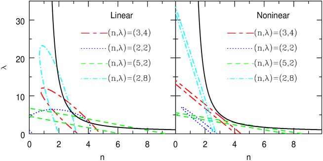
Figure 4: Left panel: The $1$-sigma contour in the $(n-\lambda)$ plane. The linear modeling for $P_{\rm mass}(k,z)$ in the range of $10\leq l\leq 10^{3}$ is used. The target modes are $(n,\lambda)=(3,4),(2,2),(5,2)$, and $(2,8)$, respectively. The other target parameters are $w_{0}=-1,~{}w_{a}=0,~{}\Omega_{0}=0.28,~{}\Omega_{b}=0.044,~{}h=0.7,\sigma_{8}=0.8$, and $n_{s}=0.95$. The solid curve corresponds to $k_{C}=0.2h{\rm Mpc}^{-1}$. Right panel: Same as the left panel, but with the nonlinear modeling for $P_{\rm mass}(k,z)$ of the range of $10\leq l\leq 3\times 10^{3}$.

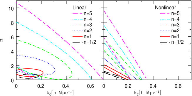
Figure 5: Left panel: The $1$-sigma contour in the $(k_{C}-n)$ plane. The linear modeling for $P_{\rm mass}(k,z)$ in the range of $10\leq l\leq 10^{3}$ is used. We assume the target modes $k_{C}=0.1h{\rm Mpc}^{-1}$ and $n=5,~{}4,~{}3,~{}2,~{}1$, and $1/2$, respectively, from the larger circle to smaller one. The other parameters are the same as those of Fig. 4. Right panel: Same as the left panel, but with the nonlinear modeling for $P_{\rm mass}(k,z)$ of the range of $10\leq l\ \leq 3\times 10^{3}$.

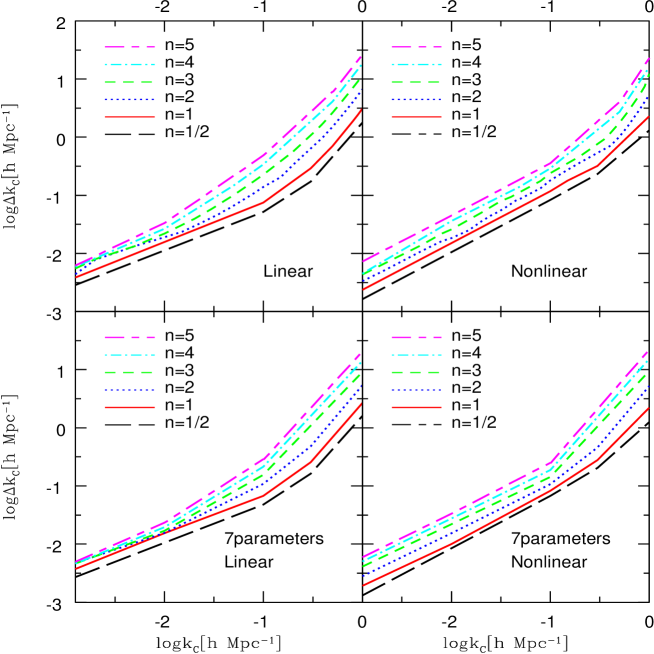
Figure 6: The 1-sigma error on $k_{C}$ as a function of the target value of $k_{C}$, where the other parameters are marginalized over. The left (right) panels use the linear (nonlinear) modeling for $P_{\rm mass}(k,z)$ of the range of $10\leq l\leq 10^{3}$ ($10\leq l\ \leq 3\times 10^{3}$). In each panel, the curves assume the target parameter $n=5,~{}4,~{}3,~{}2,~{}1$, and $1/2$, from the top to the bottom, respectively. The other target parameters are the same as those of Fig. 4. The upper panels are the result of the $9$ parameters, $k_{C}$, $n$, $w_{0},~{}w_{a},~{}\Omega_{0},~{}\Omega_{b},~{}h,~{}A,$ and $n_{s}$. The lower panels are the result of the $7$ parameters, $k_{C}$, $n$, $\Omega_{0},~{}\Omega_{b},~{}h,~{}A,$ and $n_{s}$, where the background expansion is fixed as that of the $\Lambda$CDM model.

In the Fisher matrix analysis, we assume the galaxy sample of a survey with the number density $N_{g}=35$ per arcmin.², the mean redshift $z_{m}=0.9$, and the total survey area, $\Delta A=2\times 10^{4}$ square degrees. We also assumed the tomography with $4$ redshift bins (see also Appendix). Figure 4 is the result of the Fisher matrix analysis of the $9$ parameters, $n$, $\lambda$, $w_{0},~{}w_{a},~{}\Omega_{0},~{}\Omega_{b},~{}h,~{}A,$ and $n_{s}$. Figure 4 plots the $1$-sigma contour in the $n-\lambda$ plane, which is obtained by marginalizing the Fisher matrix over the other 7 parameters. The target values of $n$ and $\lambda$ are shown in the panels. The other target parameters are $w_{0}=-1,~{}w_{a}=0,~{}\Omega_{0}=0.28,~{}\Omega_{b}=0.044,~{}h=0.7$, $n_{s}=0.95$, and $A$ which is set so that $\sigma_{8}=0.8$. We take into account the Planck prior constraint of the expected errors $\Delta w_{0}=0.6,~{}\Delta w_{a}=1.9,~{}\Delta\Omega_{0}=0.01,~{}\Delta\Omega_{b}=0.0014,~{}\Delta h=0.01,~{}\Delta\sigma_{8}=0.1$ and $\Delta n_{s}=0.014$ Kitching08 . The left panel shows the result using the linear theory for the matter power spectrum of the range, $10\leq l\leq 10^{3}$. The right panel is the result with the nonlinear matter power spectrum of the range, $10\leq l\leq 3\times 10^{3}$. In this figure, the solid curve corresponds to $k_{C}=0.2~{}h{\rm Mpc}^{-1}$, which was defined as the boundary between the general-relativity regime and the dispersion regime in the reference Tsujikawa09 .

Figure 5 is similar to Fig. 4, but the $1$-sigma contour in the $k_{C}-n$ plane. We assumed the target modes $k_{C}=0.1h{\rm Mpc}^{-1}$ and $n=5,~{}4,~{}3,~{}2,~{}1$, and $1/2$, from the larger circle to smaller one, respectively. The other parameters are the same as those of Fig. 4. Figure 6 shows the $1$-sigma error on $k_{C}$ as a function of the target value of $k_{C}$, where the other parameters are marginalized over. The left panels are the linear theory, while the right panels are the nonlinear model. The upper panels are the result of the Fisher matrix of the $9$ parameters $n$, $k_{C}$, $w_{0},~{}w_{a},~{}\Omega_{0},~{}\Omega_{b},~{}h,~{}A,$ and $n_{s}$. Then, the $1$-sigma error $\Delta k_{C}$ is evaluated by marginalizing the Fisher matrix over the 8 parameters $n,~{}w_{0},~{}w_{a},~{}\Omega_{0},~{}\Omega_{b},~{}h,~{}A,$ and $n_{s}$. The error of $k_{C}$ is the same order of $k_{C}$ for the cases $n=1/2$ and $1$, but the error becomes larger as $n$ becomes larger. The lower panels are the result of the Fisher matrix of the $7$ parameters, $k_{C}$, $n$, $\Omega_{0},~{}\Omega_{b},~{}h,~{}A,$ and $n_{s}$, with fixing the background expansion to be that of the $\Lambda$CDM model. Thus, the inclusion of the parameters $w_{0}$ and $w_{a}$ does not alter the result qualitatively.

Figures 4-6 show that the difference between the linear modeling and the nonlinear modeling is not very significant. We adopted the Peacock and Dodds formula PeacockDodds96 for the nonlinear modeling of the matter power spectrum, while the formula by Smith et al. Smith03 has been used frequently Oyaizu08a ; Oyaizu08b ; Schmidt09a ; Koyama09 ; Beynon09 . However, the choice of the nonlinear formula doesn’t alter our conclusion qualitatively. We have not taken the nonlinear effect from the Chameleon mechanism into account. The nonlinear modeling for the $f(R)$ model has not been studied well for the general case of $n$. The effect of the nonlinear modeling might need further investigations.

V summary and conclusions

In the present paper, we have investigated the linear growth rate of cosmological matter density perturbations in the viable $f(R)$ model both numerically and analytically. We found that the growth rate in the scalar-tensor regime can be characterized by a simple analytic formula (15). This is useful to understand the characteristic behavior of the growth index in the scalar-tensor regime. We also investigate a prospect of constraining the Compton wavelength scale of the $f(R)$ model with a future weak lensing survey. This result shows that a constraint on $k_{C}$ of the same order of $k_{C}$ will be obtained for the model $n=1$ and $n=1/2$, though the constraint is weaker as $n$ is larger. For $k_{C}\lower 2.15277pt\hbox{$\;\buildrel>\over{\sim}\;$}1h{\rm Mpc}^{-1}$, the constraint is very weak. This is because the weak lensing statistics is not very sensitive to the density perturbations on the smaller scales.

Finally we mention about the effect of the late-time evolution of matter density perturbations in the $f(R)$ model on the spectral index. This effect causes the additional spectral index, which is evaluated by $\Delta n_{s}={d\ln D_{1}^{2}(a,k)/d\ln k}$. The analytic formula of the additional spectral index is given by Starobinsky Starobinsky07 (see also Tsujikawa08 ; Motohashi ), $\Delta n_{s}={(\sqrt{33}-5)/(6n+4)}$, which yields $\Delta n_{s}=0.11,~{}0.074,~{}0.047,~{}0.034,~{}0.027$, and $0.022$, for $n=1/2,~{}1,~{}2,~{}3,~{}4$, and $5$, respectively. Figure 7 plots our numerical result of $\Delta n_{s}$ as a function of $k$ assuming $k_{C}=0.1h{\rm Mpc}^{-1}$. The numerical result approaches the analytic result at $k\gg k_{C}$, but one can see the bump around the wavenumber $k_{C}$, depending on $n$. Possibility of detecting of the spectral shape is interesting, but is out of the scope of this paper.

Figure 7: The additional spectral index $\Delta n_{s}$ as a function of wavenumber $k(h{\rm Mpc}^{-1})$. Here we adopted $k_{C}=0.1h{\rm Mpc}^{-1}$. The curves assume $n=1/2,1,~{}2,~{}3,~{}4$, and $5$, from the top to the bottom, respectively.

Appendix A Modeling of weak lensing survey power spectrum

We briefly review the Fisher matrix analysis for a weak lensing survey. The analysis in the present paper is almost the same as that of Ref. Yamamoto07 , but the difference is the modeling for the evolution of the matter density perturbations.

As is described in Sec. IV, the signal of the weak lensing is determined by $\Phi-\Psi$ along the path of a light ray. Assuming the weak lensing tomography method WHU , the cosmic shear power spectrum for the $i$-th and $j$-th redshift bins is

$$P_{(ij)}(l)={\int }_0^{\mathrm{\infty }}𝑑\chi {\overline{W}}_i(z(\chi )){\overline{W}}_j(z(\chi )){\left(\frac{l}{\chi }\right)}^4\frac{1}{4}{P}_{\mathrm{\Phi }-\mathrm{\Psi }}(k\to \frac{l}{\chi },z(\chi )$$

References

- (1) A. G. Riess et al., Astron. J. 116, 1009 (1998)
- (2) S. Perlmutter et al., Astropys. J. 517, 565 (1999)
- (3) D. N. Spergel et al., Astropys. J. Suppl. Ser. 170, 377 (2007)
- (4) D. J. Eisenstein et al., Astrophys. J. 633, 560 (2005)
- (5) W. J. Percival et al., Mon. Not. R. Astron. Soc. 381, 1053 (2007)
- (6) S. Weinberg, Rev. Mod. Phys., 61, 1 (1989)
- (7) P. J. E. Peebles and B. Ratra, Rev. Mod. Phys. 75, 559 (2003)
- (8) E. J. Copeland, M. Sami and S. Tsujikawa, Int. J. Mod. Phys. D15, 1753 (2006)
- (9) S. M. Carroll, V. Duvvuri, M. Trodden and M. S. Turner Phys. Rev. D 70 043528 (2004)
- (10) S. Nojiri and S. D. Odintsov, Phys. Rev. D 68 123512 (2003)
- (11) S. Capozziello, S. Carloni and A. Troisi, Recent Res. Dev. Astron. Astrophys. 1, 625 (2003)
- (12) T. P. Sotiriou and V. Faraoni, arXiv:0805.1726 [Rev. Mod. Phys. (to be published)]
- (13) G R. Dvali, G. Gabadadze and M. Porrati, Phys. Lett. B 485 208 (2000)
- (14) D. Huterer and M. S. Turner, Phys. Rev. D 64, 123527 (2001)
- (15) M. Chevalier and D. Polarski, Int. J. Mod. Phys. D 10, 213 (2001)
- (16) E. V. Linder, Pys. Rev. Lett. 90, 091301 (2003)
- (17) V. Sahni, A. Shafieloo and A. A. Starobinsky, Phys. Rev. D 78, 103502 (2008)
- (18) M. Ishak, A. Upadhye and D. N. Spergel, Phys. Rev. D 74, 043513 (2006)
- (19) K. Yamamoto, D. Parkinson, T. Hamana, R.C. Nichol and Y. Suto, Phys. Rev. D 76, 023504 (2007)
- (20) D. Huterer and E. V. Linder, Phys. Rev. D 75, 023519 (2007)
- (21) M. Kunz and D. Sapone, Pys. Rev. Lett. 98, 121301 (2007)
- (22) Y.-S. Song and K. Koyama, J. Cosmol. Astropart. Phys. 01, 048 (2009)
- (23) K. Koyama, A. Taruya and T. Hiramatsu, Phys. Rev. D 79, 123512 (2009)
- (24) A. Albrecht et al., astro-ph/0609591
- (25) J. A. Frieman, M. S. Turner and D. Huterer, Ann. Rev. Astron. Astrophys. 46, 385 (2008)
- (26) http://www.sdss3.org/
- (27) H. Aihara, ”Subaru Dark Energy Survey - Hyper Suprime-Cam Project”, in IPMU international conference on Dark Energy: lighting up the darkness!, Kashiwa, Japan, 2009
- (28) http://www.lsst.org/
- (29) http://www.skatelescope.org/
- (30) M. Robberto , A.Cimatti, and the SPACE Science Team, Nuovo Cimento Soc. Ital. Fis. 122B, 1467 (2007)
- (31) http://www.darkenergysurvey.org
- (32) http://pan-starrs.ifa.hawaii.edu
- (33) http://www.ias.u-psud.fr/imEuclid
- (34) E. V. Linder, Astropart. Phys. 29, 336 (2008)
- (35) S. Nesseris and L. Perivolaropoulos, Phys. Rev. D 77, 023504 (2008)
- (36) C. Di Porto and L. Amendola, Phys. Rev. D 77, 083508 (2008)
- (37) A. F. Heavens, T. D. Kitching and L. Verde, Mon. Not. R. Astron. Soc. 380, 1029 (2007)
- (38) P. Zhang, M. Liguori, R. Bean and S. Dodelson, Phys. Rev. Lett. 99, 141302 (2007)
- (39) L. Amendola, M. Kunz and D. Sapone, J. Cosmol. Astropart. Phys. 04, 013 (2008)
- (40) F. Schmidt, Phys. Rev. D 78, 043002 (2008)
- (41) Y.-S. Song and O. Dore, J. Cosmol. Astropart. Phys. 03, 025 (2009) arXiv:0812.0002
- (42) S. Tsujikawa and T. Tatekawa, Phys. Lett. B 665, 325 (2008)
- (43) S. Thomas, A. Abdalla, B. Filipe and J. Weller, Mon. Not. R. Astron. Soc. 395, 197 (2009)
- (44) G.-B. Zhao, L. Pogosian, A. Silvestri and J. Zylberberg, Phys. Rev. D 79, 083513 (2009)
- (45) G.-B. Zhao, L. Pogosian, A. Silvestri and J. Zylberberg, Phys. Rev. Lett., 103, 241301 (2009)
- (46) J. Guzik, B. Jain and M. Takada, arXiv:0906.2221
- (47) R. Bean, arXiv:0909.3853
- (48) E. V. Linder, Phys. Rev. D 72, 043529 (2005)
- (49) L. Knox, Y.-S. Song and J.A. Tyson, Phys. Rev. D 74, 023512 (2006)
- (50) E. V. Linder and R. N. Cahn, Astropart. Phys. 28, 481 (2007)
- (51) Y. Gong, Phys. Rev. D 78, 123010 (2008)
- (52) Y. Wang, J. Cosmol. Astropart. Phys. 05, 021 (2008)
- (53) D. Polarski and R. Gannouji, Phys. Lett. B 660, 439 (2008)
- (54) G. Ballesteros and A. Riotto, Phys. Lett. B 668, 171 (2008)
- (55) R. Gannouji and D. Polarski, J. Cosmol. Astropart. Phys. 05, 018 (2008)
- (56) M. Sereno and J. A. Peacock, Mon. Not. R. Astron. Soc. 371, 719 (2006)
- (57) R. Gannouji, B. Moraes and D. Polarski, arXiv:0809.3374
- (58) E. Bertschinger and P. Zukin, Phys. Rev. D 78, 024015 (2008)
- (59) I. Laszlo and R. Bean, Phys. Rev. D 77, 024048 (2008)
- (60) H. Wei, Phys. Lett. B 664, 1 (2008)
- (61) J. B. Dent and S. Dutta, Phys. Rev. D 79, 063516 (2009)
- (62) J. B. Dent, S. Dutta and L. Perivolaropoulos, Phys. Rev. D 80, 023514 (2009)
- (63) A. A. Starobinsky, JETP Lett. 86, 157 (2007)
- (64) W. Hu and I. Sawicki, Phys. Rev. D 76, 064004 (2007)
- (65) S. A. Appleby and R. A. Battye, Pys. Lett. B 654 7 (2007)
- (66) S. Tsujikawa, Phys. Rev. D 77, 023507 (2008)
- (67) S. Tsujikawa, R. Gannouji, B. Moraes and D. Polarski, Phys. Rev. D 80, 084044 (2009)
- (68) S. Nojiri and S. D. Odintsov, Phys. Lett. B 657, 238 (2007)
- (69) S. Nojiri and S. D. Odintsov, Phys. Rev. D 77, 026007 (2008)
- (70) G. Cognola et al., Phys. Rev. D 77, 046009 (2008)
- (71) D. F. Mota and J. D. Barrow, Phys. Lett. B 581, 141 (2004)
- (72) J. Khoury, A. Weltman, Phys. Rev. D 69, 044026 (2004)
- (73) P. Brax, C. van de Bruck, A. C. Davis and D. J. Shaw, Phys. Rev. D 78, 104021 (2008)
- (74) T. Kobayashi and K. I. Maeda, Phys. Rev. D 78 064019 (2008)
- (75) A. Upadhye and W. Hu, Phys. Rev. D 80 064002 (2009)
- (76) L. Pogosian and A. Silvestri, Phys. Rev. D 77, 023503, (2008)
- (77) Y.-S. Song, W. Hu and I. Sawicki, Phys. Rev. D 75, 044004, (2007)
- (78) R. Bean, D. Bernat, L. Pogosian, A. Silvestri and M. Trodden, Phys. Rev. D 75, 064020 (2007)
- (79) S. Tsujikawa, Phys. Rev. D 76, 023514 (2007)
- (80) A. de la Cruz-Dombriz, A. Dobado and A. L. Maroto, Phys. Rev. D 77, 123515 (2008)
- (81) H. Motohashi, A. A. Starobinsky and J. Yokoyama, Int. J. Mod. Phys. D 18, 1731 (2009)
- (82) P. Zhang, Phys. Rev. D 73, 123504 (2006)
- (83) S. Capozziello, M. De Laurentis and V. Faraoni, arXiv:0909.4672
- (84) S. Carloni, E. Elizalde and S. D. Odintsov, arXiv:0907
- (85) P. Brax, C. van de Bruck, A.-C. Davis and D. Shaw, arXiv:0912.0462
- (86) After we have completed this manuscript, we noticed the paper by Brax et al.Brax09 , in which the similar formula for the growth rate in the scalar-tensor regime is presented.
- (87) F. Schmidt, A. Vikhlinin and W. Hu, Phys. Rev. D 80, 083505 (2009)
- (88) Z. Girones, A. Marchetti, O. Mena, C. Pena-Garay and N. Rius, arXiv:0912.5474
- (89) K. Yamamoto, G. Nakamura, G. Huetsi, T. Narikawa and T. Sato, (unpublished)
- (90) A. Silvestri and M. Trodden, Rep. Prog. Phys. 72, 096901 (2009)
- (91) T. D. Kitching, A. F. Heavens, L. Verde, P. Serra and A. Melchiorri, Phys. Rev. D 77, 103008 (2008)
- (92) J.A. Peacock and S.J. Dodds, Mon. Not. R. Astron. Soc. 280, L19 (1996)
- (93) R. E. Smith et al., Mon. Not. R. Astron. Soc. 341, 1311 (2003)
- (94) H. Oyaizu, Phys. Rev. D 78,123523 (2008)
- (95) H. Oyaizu, M. Lima and W. Hu, Phys. Rev. D 78, 123524 (2008)
- (96) F. Schmidt, M. Lima, H. Oyaizu and W. Hu, Phys. Rev. D 79, 083518 (2009)
- (97) E. Beynon, D. J. Bacon and K. Koyama, arXiv:0910.1480
- (98) W. Hu, Astrophys. J. 522, L21 (1999)