Direct and inverse obstacle scattering problems in a piecewise homogeneous medium

Abstract

This paper is concerned with the problem of scattering of time-harmonic acoustic waves from an impenetrable obstacle in a piecewise homogeneous medium. The well-posedness of the direct problem is established, employing the integral equation method and then used, in conjunction with the representation in a combination of layer potentials of the solution, to prove a priori estimates of solutions on some part of the interface between the layered media. The inverse problem is also considered in this paper. An uniqueness result is obtained for the first time in determining both the penetrable interface and the impenetrable obstacle with its physical property from a knowledge of the far field pattern for incident plane waves. In doing so, an important role is played by the a priori estimates of the solution for the direct problem.

1 Introduction

In this paper, we consider the problem of scattering of time-harmonic acoustic plane waves by an impenetrable obstacle in a piecewise homogeneous medium. In practical applications, the background might not be homogeneous and then may be modeled as a layered medium. A medium of this type that is a nested body consisting of a finite number of homogeneous layers occurs in various areas of applications such as radar, remote sensing, geophysics, and nondestructive testing.

To give a precise description of the problem, let $\Omega_{2}\subset{\mathbb{R}}^{3}$ denote the impenetrable obstacle which is an open bounded region with a $C^{2}$ boundary $S_{1}$ and let ${\mathbb{R}}^{3}\backslash\overline{\Omega_{2}}$ denote the the background medium which is divided by means of a closed $C^{2}$ surface $S_{0}$ into two connected domains $\Omega_{0}$ and $\Omega_{1}$ (see Figure 1). Here, $\Omega_{0}$ is the unbounded homogeneous medium and $\Omega_{1}$ is the bounded homogeneous one. We assume that the boundary $S_{1}$ of the obstacle $\Omega_{2}$ has a dissection $S_{1}=\overline{\Gamma}_{0}\cup\overline{\Gamma}_{1}$, where $\Gamma_{0}$ and $\Gamma_{1}$ are two disjoint, relatively open subsets of $S_{1}$. Furthermore, the Dirichlet and impedance boundary conditions with the surface impedance a nonnegative continuous function $\lambda\in C(\Gamma_{1})$ are specified on $\Gamma_{0}$ and $\Gamma_{1}$, respectively. Note that the case $\Gamma_{1}=\emptyset$ corresponds to a sound-soft obstacle and the case $\Gamma_{0}=\emptyset,\;\lambda=0$ leads to a Neumann boundary condition which corresponds to a sound-hard obstacle.

The scattering of time-harmonic acoustic waves in a two-layered medium in ${\mathbb{R}}^{3}$ is now modeled by the Helmholtz equation with boundary conditions on the interface $S_{0}$ and boundary $S_{1}$:

$$\Delta u+k_{0}^{2}u=0 \qquad\mbox{in}\ \Omega_{0},$$ (1.1)

$$\Delta v+k_{1}^{2}v=0 \qquad\mbox{in}\ \Omega_{1},$$ (1.2)

$$u-v=0,\;\;\frac{\partial u}{\partial\nu}-\lambda_{0}\frac{\partial v}{\partial\nu}=0 \qquad\mbox{on}\;S_{0},$$ (1.3)

$$\mathscr{B}(v)=0 \qquad\mbox{on}\;S_{1},$$ (1.4)

$$\lim_{r\rightarrow\infty}r(\frac{\partial u^{s}}{\partial r}-ik_{0}u^{s})=0 r=|x|$$ (1.5)

where $\nu$ is the unit outward normal to the interface $S_{0}$ and boundary $S_{1}$, $\lambda_{0}$ is a positive constant. Here, the total field $u=u^{s}+u^{i}$ is given as the sum of the unknown scattered wave $u^{s}$ which is required to satisfy the Sommerfeld radiation condition (1.5) and incident plane wave $u^{i}=e^{ik_{0}x\cdot d}$, where $k_{j}$ is the positive wave number given by $k_{j}=\omega_{j}/c_{j}$ in terms of the frequency $\omega_{j}$ and the sound speed $c_{j}$ in the corresponding region $\Omega_{j}\;(j=0,1)$. The distinct wave numbers $k_{j}\;(j=0,1)$ correspond to the fact that the background medium consists of two physically different materials. On the interface $S_{0}$, the so-called ”transmission condition” (1.3) is imposed, which represents the continuity of the medium and equilibrium of the forces acting on it. The boundary condition $\mathscr{B}(v)=0$ on $S_{0}$ is understood as:

$$v=0 \qquad\mbox{on}\ \Gamma_{0},$$ (1.6)

$$\frac{\partial v}{\partial\nu}+i\lambda v=0 \qquad\mbox{on}\ \Gamma_{1}.$$ (1.7)

Thus, the boundary condition (1.4) is a general and realistic one and allows that the pressure of the total wave $v$ vanishes on $\Gamma_{0}$ and the normal velocity is proportional to the excess pressure on the coated part $\Gamma_{1}$.

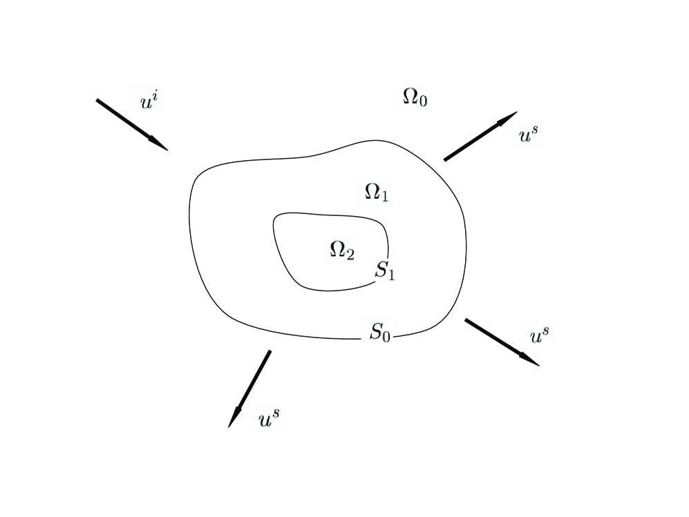
Fig. 1: Scattering in a two-layered background medium

The direct problem is to seek a pair of functions $u\in C^{2}(\Omega_{0})\cap C^{1,\alpha}(\overline{\Omega_{0}})$ and $v\in C^{2}(\Omega_{1})\cap C^{1,\alpha}(\overline{\Omega_{1}})$ satisfying (1.1)-(1.5). By the variational method, the well-posedness (existence, uniqueness and stability) of the direct problem has been established in [2] for the Dirichlet boundary condition and in [18] for a general mixed boundary condition (1.4). In the present paper, an integral equation method is employed to establish the well-posedness of the direct problem. This result is also used, in conjunction with the representation in a combination of layer potentials of the solution, to prove a priori estimates of the solution on some part of the interface $S_{0}$, which plays an important role in the proof of the uniqueness result for our inverse problem later on.

Further, it is known that $u^{s}(x)$ has the following asymptotic representation

$$u^{s}(x,d)=\frac{e^{ik_{0}|x|}}{|x|}\left\{u^{\infty}(\widehat{x},d)+O(\frac{1}{|x|})\right\}\;\mbox{as }\;|x|\rightarrow\infty$$ (1.8)

uniformly for all directions $\widehat{x}:=x/|x|$, where the function $u^{\infty}(\widehat{x},d)$ defined on the unit sphere $S$ is known as the far field pattern with $\widehat{x}$ and $d$ denoting, respectively, the observation direction and the incident direction.

The inverse problem we consider in this paper is, given the wave numbers $k_{j}$ ($j=0,1$), the positive constant $\lambda_{0}$ and the far field pattern $u^{\infty}(\widehat{x},d)$ for all incident plane waves with incident direction $d\in S$, to determine the obstacle $\Omega_{2}$ with its physical property $\mathscr{B}$ and the interface $S_{0}$. As usual in most of the inverse problems, the first question to ask in this context is the identifiability, that is, whether an inaccessible obstacle $\Omega_{2}$ with its physical property $\mathscr{B}$ and the interface $S_{0}$ can be identified from a knowledge of the far-field pattern. Mathematically, the identifiability is the uniqueness issue which is of theoretical interest and is required in order to proceed to efficient numerical methods of solutions.

Since the first uniqueness result given by Schiffer in 1967 for a sound-soft obstacle [4, 15], there has been an extensive study in this direction in the literature; see, e.g. [5, 6, 7, 8, 10, 11, 20, 22, 23, 24, 25, 26, 27] for scattering in a homogeneous medium, [9, 13, 19] for scattering in an inhomogeneous medium and [16] for scattering by special obstacles such as balls and polyhedra. However, there are few uniqueness results for inverse obstacle scattering in a piecewise homogeneous medium. For the case of a known piecewise homogeneous medium, Yan and Pang [29] established a uniqueness result for the inverse scattering problem of determining a sound-soft obstacle based on Schiffer’s idea; their method can not be extended to other boundary conditions. They obtained a uniqueness result for the case of a sound-hard obstacle in a two-layered background medium in [21] using a generalization of Schiffer’s method. However, their method is hard to be extended to the case of a multilayered background medium and seems unreasonable to require the interior wave number to be in an interval. Recently in [18], based on a generalization of the mixed reciprocity relation, we proved that both the obstacle $\Omega_{2}$ and its physical property $\mathscr{B}$ can be uniquely recovered from a knowledge of the far field pattern for incident plane waves. This seems to be appropriate for a number of applications where the physical nature of the obstacle is unknown. The tools and the uniqueness result developed in [18] can also be extended to inverse electromagnetic scattering problems [17]. For the case of an unknown piecewise homogeneous medium, Athanasiadis, Ramm and Stratis [1] and Yan [28] proved that the interfaces between the layered media can be determined uniquely by the corresponding far field pattern in the special case when the impenetrable obstacle does not exist.

However, to the authors’ knowledge, no uniqueness result is available for determining both the obstacle embedded in the piecewise homogeneous medium and the interfaces between the layered media from a knowledge of the far field pattern for incident plane waves. In this paper, we will prove for the first time that both the inaccessible obstacle $\Omega_{2}$ with its physical property $\mathscr{B}$ and the interface $S_{0}$ can be uniquely determined by a knowledge of the far-field pattern. We remark that the results obtained in this paper are also available for both the 2D case and the case of a multilayered medium and can be proved similarly.

The remaining part of the paper is organized as follows. In the next section, we will establish the well-posedness of the direct scattering problem, employing the integral equation method. With the help of the representation in a combination of layer potentials of the solution, a priori estimates of solutions are also obtained on some part of the interface between the layered media. Section 3 is devoted to the proof of the result on the unique determination of both the obstacle $\Omega_{2}$ with its physical property $\mathscr{B}$ and the surface $S_{0}$ from a knowledge of the far field pattern for incident plane waves.

2 The direct scattering problem

In this section we first establish the well-posedness of the direct problem, employing the integral equation method and then make use of the representation in a combination of layer potentials of the solution to prove some a priori estimates of the solution which plays an important role in the inverse problem. We shall use $C$ to denote a generic constant whose values may change in different inequalities but always bounded away from infinity.

As incident fields $u^{i}$, plane waves and point sources (cf. (2.7) below) are of special interest. Denote by $u^{s}(\cdot,d)$ the scattered field for an incident plane wave $u^{i}(\cdot,d)$ with incident direction $d\in S$ and by $u^{\infty}(\cdot,d)$ the corresponding far field pattern. The scattered field for an incident point source $\Phi(\cdot,z)$ with source point $z\in{\mathbb{R}}^{3}$ is denoted by $u^{s}(\cdot;z)$ and the corresponding far field pattern by $\Phi^{\infty}(\cdot,z)$.

The direct problem is to look for a pair of functions $u\in C^{2}(\Omega_{0})\cap C^{1,\alpha}(\overline{\Omega_{0}})$ and $v\in C^{2}(\Omega_{1})\cap C^{1,\alpha}(\overline{\Omega_{1}})$ satisfying the following boundary value problem:

$$\Delta u+k_{0}^{2}u=0 \qquad\mbox{in}\ \Omega_{0},$$ (2.1)

$$\Delta v+k_{1}^{2}v=0 \qquad\mbox{in}\ \Omega_{1},$$ (2.2)

$$u-v=f,\;\;\frac{\partial u}{\partial\nu}-\lambda_{0}\frac{\partial v}{\partial\nu}=g \qquad\mbox{on}\;S_{0},$$ (2.3)

$$v=0 \qquad\mbox{on}\ \Gamma_{0},$$ (2.4)

$$\frac{\partial v}{\partial\nu}+i\lambda v=0 \qquad\mbox{on}\ \Gamma_{1},$$ (2.5)

$$\lim_{r\rightarrow\infty}r(\frac{\partial u}{\partial r}-ik_{0}u)=0, r=|x|.$$ (2.6)

Here, we assume that $k_{0},k_{1}$ and $\lambda_{0}$ are given positive constants and that $f\in C^{1,\alpha}(S_{0})$ and $g\in C^{0,\alpha}(S_{0})$ are given functions in Hölder spaces with exponent $0<\alpha<1$.

Remark 1.

The problem of scattering of the incident plane wave $\displaystyle u^{i}=e^{ik_{0}x\cdot d}$ is a particular case of the problem (2.1)-(2.6). In particular, the scattered field $u^{s}$ satisfies the problem (2.1)-(2.6) with $\displaystyle u=u^{s},\;f=-u^{i}|_{S_{0}},\;g=-\frac{\partial u^{i}}{\partial\nu}|_{S_{0}}$.

The following uniqueness result has been established in [18] (see Theorem 2.3 of [18]).

Theorem 2.

The boundary value problem $(\ref{HE0})-(\ref{rc})$ admits at most one solution.

Denote by $\Phi_{j}$ the fundamental solution of the Helmholtz equation with wave number $k_{j}\;(j=0,1)$, which is given by

$$\Phi_{j}(x,y)=\frac{e^{ik_{j}|x-y|}}{4\pi|x-y|},\qquad\ x,y\in{\mathbb{R}}^{3},x\neq y.$$ (2.7)

For $i,j=0,1$ define the single- and double-layer operators $S_{i,j}$ and $K_{i,j}$, respectively, by

$$(S_{i,j}\phi)(x):=\int_{S_{0}}\Phi_{j}(x,y)\phi(y)ds(y)\qquad \;x\in S_{i},$$

$$(K_{i,j}\phi)(x):=\int_{S_{0}}\frac{\partial\Phi_{j}(x,y)}{\partial\nu(y)}\phi(y)ds(y)\qquad \;x\in S_{i}$$

and the normal derivative operators $K^{{}^{\prime}}_{i,j}$ and $T_{i,j}$ by

$$(K^{{}^{\prime}}_{i,j}\phi)(x):=\frac{\partial}{\partial\nu(x)}\int_{S_{0}}\Phi_{j}(x,y)\phi(y)ds(y)\qquad \;x\in S_{i},$$

$$(T_{i,j}\phi)(x):=\frac{\partial}{\partial\nu(x)}\int_{S_{0}}\frac{\partial\Phi_{j}(x,y)}{\partial\nu(y)}\phi(y)ds(y)\qquad \;x\in S_{i}.$$

For $i,j=0,1$ define the single- and double-layer operators $\widetilde{S}_{i,j}$ and $\widetilde{K}_{i,j}$, respectively, by

$$(\widetilde{S}_{i,j}\phi)(x):=\int_{\Gamma_{j}}\Phi_{1}(x,y)\phi(y)ds(y)\qquad \;x\in S_{i},$$ (2.8)

$$(\widetilde{K}_{i,j}\phi)(x):=\int_{\Gamma_{j}}\frac{\partial\Phi_{1}(x,y)}{\partial\nu(y)}\phi(y)ds(y)\qquad \;x\in S_{i}$$ (2.9)

and the normal derivative operators $\widetilde{K}^{{}^{\prime}}_{i,j}$ and $\widetilde{T}_{i,j}$ by

$$(\widetilde{K}^{{}^{\prime}}_{i,j}\phi)(x):=\frac{\partial}{\partial\nu(x)}\int_{\Gamma_{j}}\Phi_{1}(x,y)\phi(y)ds(y)\qquad \;x\in S_{i},$$

$$(\widetilde{T}_{i,j}\phi)(x):=\frac{\partial}{\partial\nu(x)}\int_{\Gamma_{j}}\frac{\partial\Phi_{1}(x,y)}{\partial\nu(y)}\phi(y)ds(y)\qquad \;x\in S_{i}.$$

For the mapping properties of these operators in the spaces of continuous and Hölder continuous functions we refer to Section 3.1 in [4] or Chapter 2 in [3].

Theorem 3.

The boundary value problem $(\ref{HE0})-(\ref{rc})$ has a unique solution. Moreover, there exists a positive constant $C=C(\lambda_{0},\Omega_{1},\alpha)$ such that

$$\|u\|_{C^{1,\alpha}(\overline{\Omega_{0}})}+\|v\|_{C^{1,\alpha}(\overline{\Omega_{1}})}\leq C(\|f\|_{C^{1,\alpha}(S_{0})}+\|g\|_{C^{0,\alpha}(S_{0})}).$$ (2.10)

Proof.

The uniqueness of solutions follows from Theorem 2. We now prove the existence of solutions by using the integral equation method. Following [3] and [4] we seek a solution in the form

$$u(x) = \int_{S_{0}}\left\{\lambda_{0}\frac{\partial\Phi_{0}(x,y)}{\partial\nu(y)}\psi(y)+\Phi_{0}(x,y)\phi(y)\right\}ds(y)\hskip 17.07182pt\qquad x\in\Omega_{0},\qquad$$ (2.11)

$$v(x) = \int_{S_{0}}\left\{\frac{\partial\Phi_{1}(x,y)}{\partial\nu(y)}\psi(y)+\Phi_{1}(x,y)\phi(y)\right\}ds(y)$$ (2.12)

$$+\int_{\Gamma_{0}}\left\{\frac{\partial\Phi_{1}(x,y)}{\partial\nu(y)}\chi(y)-i\eta\Phi_{1}(x,y)\chi(y)\right\}ds(y)$$

$$+\int_{\Gamma_{1}}\left\{\Phi_{1}(x,y)\varphi(y)+i\eta\frac{\partial\Phi_{1}(x,y)}{\partial\nu(y)}(\widetilde{S}^{2}\varphi)(y))\right\}ds(y)\qquad x\in\Omega_{1}$$

with four densities $\psi\in C^{1,\alpha}(S_{0})$, $\phi\in C^{0,\alpha}(S_{0})$, $\chi\in C^{1,\alpha}(\Gamma_{0})$, $\varphi\in C^{1,\alpha}(\Gamma_{1})$ and a real coupling parameter $\eta\neq 0$. By $\widetilde{S}$ we denote the single-layer operator (2.8) in the potential theoretic limit case $k_{1}=0$. Then from the jump relations we see that the potentials $u$ and $v$ defined above solve the boundary value problem $(\ref{HE0})-(\ref{rc})$ provided the densities $\psi,\phi,\chi,\varphi$ satisfy the system of integral equations

$$\psi+\mu(\lambda_{0}K_{0,0}-K_{0,1})\psi+\mu(S_{0,0}-S_{0,1})\phi$$

$$\qquad\qquad\qquad\qquad\qquad-\mu(\widetilde{K}_{0,0}-i\eta\widetilde{S}_{0,0})\chi+M_{1}\varphi=\mu f\quad\mbox{on}\;\;S_{0},$$ (2.13)

$$\phi-\mu\lambda_{0}(T_{0,0}-T_{0,1})\psi-\mu(K^{{}^{\prime}}_{0,0}-\lambda_{0}K^{{}^{\prime}}_{0,1})\phi$$

$$\qquad\qquad\qquad\qquad-\mu\lambda_{0}(T_{0,0}-i\eta K^{{}^{\prime}}_{0,0})\chi+M_{2}\varphi=-\mu g\quad\mbox{on}\;\;S_{0},$$ (2.14)

$$\chi+2K_{1,1}\psi+2S_{1,1}\phi+2(\widetilde{K}_{1,0}-i\eta\widetilde{S}_{1,0})\chi+M_{3}\varphi=0\quad\mbox{on}\;\;\Gamma_{0},$$ (2.15)

$$\varphi-2(T_{1,1}+i\lambda K_{1,1})\psi-2(K^{{}^{\prime}}_{1,1}+i\lambda S_{1,1})\phi+M_{4}\chi+M_{5}\varphi=0\quad\mbox{on}\;\;\Gamma_{1}$$ (2.16)

with $\mu={2}/({\lambda_{0}+1})$, where

$$M_{1} = -\mu(\widetilde{S}_{0,1}+i\eta\widetilde{K}_{0,1}\widetilde{S}^{2}),$$

$$M_{2} = -\mu(\widetilde{K}^{{}^{\prime}}_{0,1}+i\eta\widetilde{T}_{0,1}\widetilde{S}^{2}),$$

$$M_{3} = 2(\widetilde{S}_{1,1}+i\eta\widetilde{K}_{1,1}\widetilde{S}^{2}),$$

$$M_{4} = -2(\widetilde{T}_{1,0}-i\eta\widetilde{K}^{{}^{\prime}}_{1,0}+i\lambda\widetilde{K}_{1,0}+\lambda\eta\widetilde{S}_{1,0}),$$

$$M_{5} = -2(\widetilde{K}_{1,1}+i\eta\widetilde{T}_{1,1}\widetilde{S}^{2}-\lambda\eta\widetilde{S}^{2}+i\lambda\widetilde{S}_{1,1}-\lambda\eta\widetilde{K}_{1,1}\widetilde{S}^{2}).$$

Define the product space $X:=C^{1,\alpha}(S_{0})\times C^{0,\alpha}(S_{0})\times C^{1,\alpha}(\Gamma_{0})\times C^{1,\alpha}(\Gamma_{1})$ and introduce the operator $A:X\rightarrow X$ given by

$$A:=\left(\begin{matrix}\mu(\lambda_{0}K_{0,0}-K_{0,1})&\mu(S_{0,0}-S_{0,1})&-\mu(\widetilde{K}_{0,0}-i\eta\widetilde{S}_{0,0})&M_{1}\\ -\mu\lambda_{0}(T_{0,0}-T_{0,1})&-\mu(K^{{}^{\prime}}_{0,0}-\lambda_{0}K^{{}^{\prime}}_{0,1})&-\mu\lambda_{0}(T_{0,0}-i\eta K^{{}^{\prime}}_{0,0})&M_{2}\\ 2K_{1,1}&2S_{1,1}&2(\widetilde{K}_{1,0}-i\eta\widetilde{S}_{1,0})&M_{3}\\ -2(T_{1,1}+i\lambda K_{1,1})&-2(K^{{}^{\prime}}_{1,1}+i\lambda S_{1,1})&M_{4}&M_{5}\end{matrix}\right)$$

The operator $A$ is compact since all its entries are compact. The system (2.13)-(2.16) can be rewritten in the abbreviated form

$$(I+A)U=R,$$ (2.17)

where $I$ is the identity operator, $U=(\psi,\phi,\chi,\varphi)^{T}$ and $R=(\mu f,-\mu g,0,0)^{T}$. Thus, the Riesz-Fredholm theory is applicable. We now prove the uniqueness of solutions to the system (2.17). To this end, let $U$ be a solution of the homogeneous system corresponding to (2.17) (that is, the system (2.17) with $R=0$). Then it is enough to show that $U=0$.

We first prove that $\chi=0$ on $\Gamma_{0}$ and $\varphi=0$ on $\Gamma_{1}$. From the system (2.17) or (2.13)-(2.16) with $\mu f=-\mu g=0$ (since $R=0$) it is known that $u$ and $v$ defined in (2.11) and (2.12) satisfy the problem $(\ref{HE0})-(\ref{rc})$ with $f=g=0$. Thus, by the uniqueness Theorem 2, $u=0$ in $\Omega_{0}$ and $v=0$ in $\Omega_{1}$. Note that $v$, given by (2.12), can also be defined for $x\in\Omega_{2}$ and satisfies the Helmholtz equation $\Delta v+k_{1}^{2}v=0$ in $\Omega_{2}$. Then the jump relations yield that

$$-v_{-}=\chi,\;-\frac{\partial v_{-}}{\partial\nu}=i\eta\chi\qquad\mbox{on}\;\Gamma_{0},$$

$$-v_{-}=i\eta\widetilde{S}^{2}\varphi,\;-\frac{\partial v_{-}}{\partial\nu}=-\varphi\qquad\mbox{on}\;\Gamma_{1}.$$

Interchanging the order of integration and using Green’s first theorem over $\Omega_{2}$, we obtain

$$i\eta\left\{\int_{\Gamma_{0}}|\chi|^{2}ds+\int_{\Gamma_{1}}|\widetilde{S}\varphi|^{2}ds\right\} = i\eta\left\{\int_{\Gamma_{0}}|\chi|^{2}ds+\int_{\Gamma_{1}}\varphi\widetilde{S}^{2}\overline{\varphi}ds\right\}$$

$$= \int_{\Gamma_{0}}\overline{v_{-}}\frac{\partial v_{-}}{\partial\nu}ds+\int_{\Gamma_{1}}\overline{v}_{-}\frac{\partial v_{-}}{\partial\nu}ds$$

$$= \int_{\Omega_{2}}{|\nabla v|^{2}-k^{2}_{1}|v|^{2}}dx.$$

Taking the imaginary part of this equation gives that $\chi=0$ on $\Gamma_{0}$ and $\widetilde{S}\varphi=0$ on $\Gamma_{1}$. The single-layer potential

$$w(x):=\int_{\Gamma_{1}}\frac{1}{4\pi|x-y|}\varphi(y)ds(y)$$

with density $\varphi$ is continuous throughout ${\mathbb{R}}^{3}$, harmonic in ${\mathbb{R}}^{3}\backslash\Gamma_{1}$ and vanishes on $\Gamma_{1}$ and at infinity. Therefore, by the maximum-minimum principle for harmonic functions, we have $w=0$ in ${\mathbb{R}}^{3}$ and the jump relation yields $\varphi=0$.

Now the system (2.17) becomes

$$\left[I+\left(\begin{matrix}\mu(\lambda_{0}K_{0,0}-K_{0,1})&\mu(S_{0,0}-S_{0,1})\\ -\mu\lambda_{0}(T_{0,0}-T_{0,1})&-\mu(K^{{}^{\prime}}_{0,0}-\lambda_{0}K^{{}^{\prime}}_{0,1})\end{matrix}\right)\right]\left(\begin{matrix}\psi\\ \phi\end{matrix}\right)=\left(\begin{matrix}0\\ 0\end{matrix}\right).$$

Define

$$\widetilde{v}(x) := \int_{S_{0}}\left\{\frac{\partial\Phi_{1}(x,y)}{\partial\nu(y)}\psi(y)+\Phi_{1}(x,y)\phi(y)\right\}ds(y),\qquad x\in\Omega_{0},$$

$$\widetilde{u}(x) := -\int_{S_{0}}\left\{\frac{\partial\Phi_{0}(x,y)}{\partial\nu(y)}\psi(y)+\frac{1}{\lambda_{0}}\Phi_{0}(x,y)\phi(y)\right\}ds(y),\qquad x\in{\mathbb{R}}^{3}\backslash\overline{\Omega}_{0}.$$

Then by the jump relations for single- and double-layer potentials we have

$$\widetilde{v}-v=\psi, \;\;\;\frac{1}{\lambda_{0}}u+\widetilde{u}=\psi\qquad\mbox{on}\;\;S_{0},$$ (2.18)

$$\frac{\partial\widetilde{v}}{\partial\nu}-\frac{\partial v}{\partial\nu}=-\phi, \;\;\;\frac{\partial u}{\partial\nu}+\lambda_{0}\frac{\partial\widetilde{u}}{\partial\nu}=-\phi\qquad\mbox{on}\;\;S_{0}.$$ (2.19)

Hence, $\widetilde{v}$ and $\widetilde{u}$ solve the homogeneous transmission problem

$$\Delta\widetilde{v}+k_{1}^{2}\widetilde{v}=0\;\;\mbox{in}\;\;\Omega_{0},\qquad\Delta\widetilde{u}+k_{0}^{2}\widetilde{u}=0\;\;\mbox{in}\;\;{\mathbb{R}}^{3}\backslash\overline{\Omega}_{0}$$

with the transmission conditions (noting that $u=0$ in $\Omega_{0}$ and $v=0$ in $\Omega_{1}$)

$$\widetilde{v}-\widetilde{u}=0,\qquad\frac{\partial\widetilde{v}}{\partial\nu}=\lambda_{0}\frac{\partial\widetilde{u}}{\partial\nu}\;\;\mbox{on}\;\;S_{0}.$$

Arguing similarly as in the proof of Theorem 2.3 in [18] we can show that $\widetilde{v}=0$ in $\Omega_{0}$ and $\widetilde{u}=0$ in ${\mathbb{R}}^{3}\backslash\overline{\Omega_{0}}$. Hence we conclude from (2.18) and (2.19) that $\psi=\phi=0$ on $S_{0}$.

Thus, the injectivity of the operator $I+A$ is proved, and by the Riesz-Fredholm theory $(I+A)^{-1}$ exists and is bounded in $X$. From this we deduce that

$$\|\psi\|_{C^{1,\alpha}(S_{0})}+\|\phi\|_{C^{0,\alpha}(S_{0})}+\|\chi\|_{C^{1,\alpha}(\Gamma_{0})}+\|\varphi\|_{C^{1,\alpha}(\Gamma_{1})}$$

$$\qquad\qquad\qquad\leq C(\|f\|_{C^{1,\alpha}(S_{0})}+\|g\|_{C^{0,\alpha}(S_{0})}).$$

The estimate (2.10) follows from (2.11), (2.12) and Theorem 3.3 in [4]. ∎

We now make use of the representation (2.12) of the solution $v$ to derive an a priori estimate of the solution $v$ on some part of $S_{0}$, which is necessary in proving the uniqueness result for the inverse problem in the next section.

Let $x^{\ast}\in S_{0}$ be an arbitrarily fixed point and let us introduce the space $C_{0}(S_{0})$ which consists of all continuous functions $h\in C(S_{0}\backslash\{x^{\ast}\})$ with the property that

$$\lim_{x\rightarrow x^{\ast}}[|x-x^{\ast}|h(x)]$$

exists. It can easily be seen that $C_{0}(S_{0})$ is a Banach space equipped with the weighted maximum norm

$$\|h\|_{C_{0}(S_{0})}:=\sup_{x\neq x^{\ast},x\in S_{0}}|(x-x^{\ast})h(x)|.$$

Lemma 4.

Given two functions $f\in C^{1,\alpha}(S_{0})$ and $g\in C^{0,\alpha}(S_{0})$. Let $u\in C^{2}(\Omega_{0})\cap C^{1,\alpha}(\overline{\Omega_{0}})$ and $v\in C^{2}(\Omega_{1})\cap C^{1,\alpha}(\overline{\Omega_{1}})$ be the solution of the problem $(\ref{HE0})-(\ref{rc}).$ Let $x^{\ast}\in S_{0}$ and let $B_{1},$ $B_{2}$ be two small balls with center $x^{\ast}$ and radii $r_{1},\;r_{2}$, respectively, satisfying that $r_{1}<r_{2}$. Then there exists a constant $C>0$ such that

$$\|v\|_{\infty,S_{0}\backslash B_{2}}+\left\|\frac{\partial v}{\partial\nu}\right\|_{\infty,S_{0}\backslash B_{2}}$$

$$\qquad\qquad\leq C(\|f\|_{C_{0}(S_{0})}+\|g\|_{C_{0}(S_{0})}+\|f\|_{1,\alpha,S_{0}\backslash B_{1}}+\|g\|_{0,\alpha,S_{0}\backslash B_{1}})$$

Proof.

We consider again the system (2.17) of the boundary integral equations derived from the boundary value problem (2.1)-(2.6). In addition to the space $X$, we also consider the weighted spaces $C_{0}:=C_{0}(S_{0})\times C_{0}(S_{0})\times C^{1,\alpha}(\Gamma_{0})\times C^{1,\alpha}(\Gamma_{1})$. The matrix operator $A$ is also compact in $C_{0}$ since all entries of $A$ are compact (see [12, 13]). From the proof of Theorem 3, we know that the operator $I+A$ has a trivial null space in $X$. Therefore, by the Fredholm alternative applied to the dual system $\langle X,C_{0}\rangle$ with the $L^{2}$ bilinear form, the adjoint operator $I+A^{\prime}$ has a trivial null space in $C_{0}$. By the Fredholm alternative again, but now applied to the dual system $\langle C_{0},C_{0}\rangle$ with the $L^{2}$ bilinear form, the operator $I+A$ also has a trivial null space in $C_{0}$. Hence, by the Riesz-Fredholm theory, the system (2.17) is also uniquely solvable in $C_{0}$, and the solution depends continuously on the right-hand side:

$$\|\psi\|_{C_{0}(S_{0})}+\|\phi\|_{C_{0}(S_{0})}+\|\chi\|_{C^{1,\alpha}(\Gamma_{0})}+\|\varphi\|_{C^{1,\alpha}(\Gamma_{1})}$$

$$\qquad\qquad\qquad\leq C(\|f\|_{C_{0}(S_{0})}+\|g\|_{C_{0}(S_{0})}).$$ (2.20)

From (2.12) and the jump relation we find that on $S_{0},$

$$v=-\frac{1}{2}\psi+K_{0,1}\psi+S_{0,1}\phi+(\widetilde{K}_{0,0}-i\eta\widetilde{S}_{0,0})\chi+(\widetilde{S}_{0,1}+i\eta\widetilde{K}_{0,1}\widetilde{S}^{2})\varphi.$$ (2.21)

Thus we have

$$\|v\|_{\infty,S_{0}\backslash B_{2}} \leq C(\|\psi\|_{\infty,S_{0}\backslash B_{2}}+\|K_{0,1}\psi\|_{\infty,S_{0}\backslash B_{2}}+\|S_{0,1}\phi\|_{\infty,S_{0}\backslash B_{2}}$$ (2.22)

$$+\|(\widetilde{K}_{0,0}-i\eta\widetilde{S}_{0,0})\chi\|_{\infty,S_{0}\backslash B_{2}}+\|(\widetilde{S}_{0,1}+i\eta\widetilde{K}_{0,1}\widetilde{S}^{2})\varphi\|_{\infty,S_{0}\backslash B_{2}})$$

$$\leq C(\|\psi\|_{C_{0}(S_{0})}+\|K_{0,1}\psi\|_{\infty,S_{0}\backslash B_{2}}+\|S_{0,1}\phi\|_{\infty,S_{0}\backslash B_{2}}$$

$$+\|\chi\|_{C^{1,\alpha}(\Gamma_{0})}+\|\varphi\|_{C^{1,\alpha}(\Gamma_{1})}).$$

We choose a function $\rho_{1}\in C^{2}(S_{0})$ such that $\rho_{1}(x)=0$ for $x\in S_{0}\backslash B_{1}$ and $\rho_{1}(x)=1$ in the neighborhood of $x^{\ast}$. We also choose another function $\rho_{2}\in C^{2}(S_{0})$ such that $\rho_{2}(x)=1$ for $x\in S_{0}\backslash B_{2}$ and $\rho_{2}(x)=0$ in the neighborhood of $B_{1}$. Multiplying $K_{0,1}\psi$ by $\rho_{2}$ and splitting $\psi$ up in the form $\psi=\rho_{1}\psi+(1-\rho_{1})\psi$, we have

$$\|K_{0,1}\psi\|_{\infty,S_{0}\backslash B_{2}} = \|\rho_{2}K_{0,1}\psi\|_{\infty,S_{0}\backslash B_{2}}$$ (2.23)

$$\leq C(\|\rho_{2}K_{0,1}\rho_{1}\psi\|_{\infty,S_{0}\backslash B_{2}}+\|K_{0,1}(1-\rho_{1})\psi\|_{\infty,S_{0}\backslash B_{2}})$$

The first term on the right-hand side of the above inequality contains only an operator with a kernel vanishing in a neighborhood of the diagonal $x=y$, and therefore we have

$$\|\rho_{2}K_{0,1}\rho_{1}\psi\|_{\infty,S_{0}\backslash B_{2}}\leq C\|\psi\|_{C_{0}(S_{0})}.$$ (2.24)

Since the operator $K_{0,1}$ mapping $C(S_{0})$ into $C^{0,\alpha}(S_{0})$ is bounded (see [4]), we find, on noting that $1-\rho_{1}$ vanishes in a neighborhood of $x^{\ast}$, that

$$\|K_{0,1}(1-\rho_{1})\psi\|_{\infty,S_{0}\backslash B_{2}}\leq C\|(1-\rho_{1})\psi\|_{\infty,S_{0}\backslash B_{2}}\leq C\|\psi\|_{C_{0}(S_{0})}.$$ (2.25)

From (2.23)-(2.25) it follows that

$$\|K_{0,1}\psi\|_{\infty,S_{0}\backslash B_{2}}\leq C\|\psi\|_{C_{0}(S_{0})}.$$ (2.26)

A similar argument as above gives that

$$\|S_{0,1}\phi\|_{\infty,S_{0}\backslash B_{2}}\leq C\|\phi\|_{C_{0}(S_{0})}.$$ (2.27)

Combining (2.26)-(2.27) with (2.20) and (2.22) yields

$$\|v\|_{\infty,S_{0}\backslash B_{2}}\leq C(\|f\|_{C_{0}(S_{0})}+\|g\|_{C_{0}(S_{0})}).$$ (2.28)

Before proceeding to estimate ${\partial v}/{\partial\nu}$ we establish the following estimate in the spaces of Hölder continuous functions for $(\psi,\phi,\chi,\varphi)$:

$$\|\psi\|_{C^{1,\alpha}(S_{0}\backslash B_{3})}+\|\phi\|_{C^{0,\alpha}(S_{0}\backslash B_{3})}+\|\chi\|_{C^{0,\alpha}(\Gamma_{0})}+\|\varphi\|_{C^{0,\alpha}(\Gamma_{1})}$$

$$\qquad\leq C(\|f\|_{C_{0}(S_{0})}+\|g\|_{C_{0}(S_{0})}+\|f\|_{1,\alpha,S_{0}\backslash B_{1}}+\|g\|_{0,\alpha,S_{0}\backslash B_{1}}),$$ (2.29)

where $B_{3}$ is a ball of radius $r_{3}$ and centered at $x^{*}$ with $r_{1}<r_{3}<r_{2}$. We choose a function $\rho_{3}\in C^{2}(S_{0})$ such that $\rho_{3}(x)=0$ for $x\in S_{0}\backslash B_{2}$ and $\rho_{3}(x)=1$ in the neighborhood of $B_{3}$. We also choose another function $\rho_{4}\in C^{2}(S_{0})$ such that $\rho_{4}(x)=1$ for $x\in S_{0}\backslash B_{2}$ and $\rho_{4}(x)=0$ in the neighborhood of $B_{3}$. Splitting $U$ up in the form

$$U=\left(\begin{matrix}\rho_{3}\psi\\ \rho_{3}\phi\\ \chi\\ \varphi\end{matrix}\right)+\left(\begin{matrix}(1-\rho_{3})\psi\\ (1-\rho_{3})\phi\\ 0\\ 0\end{matrix}\right):=U_{\rho_{3}}+U_{(1-\rho_{3})}$$

and using $W_{\rho_{4}}$ to denote the matrix $W$ with its first and second rows multiplied by $\rho_{4}(x)$, it follows from (2.17) that

$$U_{\rho_{4}}=R_{\rho_{4}}-A_{\rho_{4}}U_{\rho_{3}}-A_{\rho_{4}}U_{(1-\rho_{3})}.$$ (2.30)

Arguing similarly as in deriving the estimate for $\|v\|_{\infty,S_{0}\backslash B_{2}}$ but with two different cutoff functions $\rho_{3}$ and $\rho_{4}$ replacing $\rho_{1}$ and $\rho_{2}$, we obtain from (2.30) and (2.20) that

$$\|U_{\rho_{4}}\|_{0,\alpha} = \|\psi\|_{C^{0,\alpha}(S_{0}\backslash B_{3})}+\|\phi\|_{C^{0,\alpha}(S_{0}\backslash B_{3})}+\|\chi\|_{C^{0,\alpha}(\Gamma_{0})}+\|\varphi\|_{C^{0,\alpha}(\Gamma_{1})}$$ (2.31)

$$\leq C(\|R_{\rho_{4}}\|_{0,\alpha}+\|A_{\rho_{4}}U_{\rho_{3}}\|_{0,\alpha}+\|A_{\rho_{4}}U_{(1-\rho_{3})}\|_{0,\alpha})$$

$$\leq C(\|R_{\rho_{4}}\|_{0,\alpha}+\|U\|_{C_{0}})$$

$$\leq C(\|f\|_{C_{0}(S_{0})}+\|g\|_{C_{0}(S_{0})}+\|f\|_{1,\alpha,S_{0}\backslash B_{1}}+\|g\|_{0,\alpha,S_{0}\backslash B_{1}}),$$

where $\|\cdot\|_{0,\alpha}$ and $\|\cdot\|_{C_{0}}$ denote the corresponding norms in the product spaces. Now it remains to prove the estimate of $\|\psi\|_{C^{1,\alpha}(S_{0}\backslash B_{3})}$. Multiplying (2.13) by $\rho_{4}(x)$ we obtain, on using (2.30) and noting the fact that the integral operators mapping $C^{0,\alpha}$ functions into $C^{1,\alpha}$ functions are bounded, that

$$\|\psi\|_{1,\alpha,S_{0}\backslash B_{3}} \leq \|\rho_{4}\psi\|_{1,\alpha}$$ (2.32)

$$\leq C[\|\rho_{4}(\lambda_{0}K_{0,0}-K_{0,1})\psi\|_{1,\alpha}+\|\rho_{4}(S_{0,0}-S_{0,1})\phi\|_{1,\alpha}$$

$$+\|\rho_{4}(\widetilde{K}_{0,0}-i\eta\widetilde{S}_{0,0})\chi\|_{1,\alpha}+\|\rho_{4}(\widetilde{S}_{0,1}+i\eta\widetilde{K}_{0,1}\widetilde{S}^{2})\varphi\|_{1,\alpha}+\|\rho_{4}f\|_{1,\alpha}]$$

$$\leq C[\|U\|_{C_{0}}+\|(1-\rho_{3})U\|_{0,\alpha}+\|\rho_{4}f\|_{1,\alpha}]$$

$$\leq C[\|U\|_{C_{0}}+\|\psi\|_{C^{0,\alpha}(S_{0}\backslash B_{3})}+\|\phi\|_{C^{0,\alpha}(S_{0}\backslash B_{3})}+\|\chi\|_{C^{0,\alpha}(\Gamma_{0})}$$

$$+\|\varphi\|_{C^{0,\alpha}(\Gamma_{1})}+\|f\|_{1,\alpha,S_{0}\backslash B_{3}}].$$

Combining (2.20) and (2.31)-(2.32) yields the desired estimate (2.29).

We now estimate $\displaystyle\left\|\frac{\partial v}{\partial\nu}\right\|_{0,\alpha,S_{0}\backslash B_{2}}$. From (2.12) and the jump relation it is seen that on $S_{0},$

$$\frac{\partial v}{\partial\nu}=\frac{1}{2}\phi+T_{0,1}\psi+K^{{}^{\prime}}_{0,1}\phi+(\widetilde{T}_{0,0}-i\eta\widetilde{K}^{{}^{\prime}}_{0,0})\chi+(\widetilde{K}^{{}^{\prime}}_{0,1}+i\eta\widetilde{T}_{0,1}\widetilde{S}^{2})\varphi.$$ (2.33)

Writing $\psi=\rho_{3}\psi+(1-\rho_{3})\psi$ and$\phi=\rho_{3}\phi+(1-\rho_{3})\phi$, we obtain from (2.33) that

$$\left\|\frac{\partial v}{\partial\nu}\right\|_{0,\alpha,S_{0}\backslash B_{2}} \leq \left\|\rho_{4}\frac{\partial v}{\partial\nu}\right\|_{0,\alpha,S_{0}}$$

$$\leq C[\|\psi\|_{C_{0}(S_{0})}+\|\phi\|_{C_{0}(S_{0})}+\|(1-\rho_{3})\psi\|_{1,\alpha,S_{0}}$$

$$+\|(1-\rho_{3})\phi\|_{0,\alpha,S_{0}}+\|\chi\|_{C^{0,\alpha}(\Gamma_{0})}+\|\varphi\|_{C^{0,\alpha}(\Gamma_{1})}]$$

$$\leq C[\|\psi\|_{C_{0}(S_{0})}+\|\phi\|_{C_{0}(S_{0})}+\|\psi\|_{1,\alpha,S_{0}\backslash B_{3}}+\|\phi\|_{0,\alpha,S_{0}\backslash B_{3}}$$

$$+\|\chi\|_{C^{0,\alpha}(\Gamma_{0})}+\|\varphi\|_{C^{0,\alpha}(\Gamma_{1})}].$$

Combining this with (2.20) and (2.29) yields

$$\left\|\frac{\partial v}{\partial\nu}\right\|_{0,\alpha,S_{0}\backslash B_{2}}\leq C(\|f\|_{C_{0}(S_{0})}+\|g\|_{C_{0}(S_{0})}+\|f\|_{1,\alpha,S_{0}\backslash B_{1}}+\|g\|_{0,\alpha,S_{0}\backslash B_{1}}).$$ (2.34)

This completes the proof. ∎

3 The inverse scattering problem

Following the ideas of [12] for transmission problems in a homogeneous medium and of [13] for transmission problems in an inhomogeneous medium, we prove in this section that the interface $S_{0}$ can be uniquely determined by the far field pattern. Combining this with the earlier result in [18], we have in fact proved that both the penetrable interface $S_{0}$ and the impenetrable obstacle $\Omega_{2}$ with its physical property $\mathscr{B}$ can be uniquely determined from a knowledge of far field pattern. To establish the uniqueness result for the inverse problem, we need the following two lemmas, in which $\Omega={\mathbb{R}}^{3}\backslash\Omega_{0}$ so that $\Omega_{2}\subset\Omega$ and $\widetilde{\Omega}={\mathbb{R}}^{3}\backslash\overline{\widetilde{\Omega}}_{0}$ for some domain $\widetilde{\Omega}_{0}$ with the interface $\widetilde{S}_{0}=\partial\widetilde{\Omega}_{0}\cap\partial\widetilde{\Omega}$ and with the domain $\widetilde{\Omega}_{2}\subset\widetilde{\Omega}$.

Lemma 5.

Suppose the positive numbers $k_{0}$, $k_{1}$ and $\lambda_{0}$ are given. For $\Omega_{2}\subset\Omega,\;\widetilde{\Omega}_{2}\subset\widetilde{\Omega}$ let $G$ be the unbounded component of ${\mathbb{R}}^{3}\setminus(\overline{\Omega\cup\widetilde{\Omega}})$ and let $u^{\infty}(\hat{x},d)=\widetilde{u}^{\infty}(\hat{x},d)$ for all $\hat{x},\;d\in S$ with $\widetilde{u}^{\infty}(\hat{x},d)$ being the far field pattern of the scattered field $\widetilde{u}^{s}(x,d)$ corresponding to the obstacle $\widetilde{\Omega}_{2}$, the interface $\widetilde{S}_{0}$ and the same incident plane wave $u^{i}(x,d)$. For $z\in G$ let $(u^{s},v)$ be the unique solution of the problem

$$\Delta u^{s}+k_{0}^{2}u^{s}=0 \;{\rm in}\;\Omega_{0}\setminus\{z\},$$ (3.1)

$$\Delta v+k_{1}^{2}v=0 \;{\rm in}\;\Omega_{1},$$ (3.2)

$$u^{s}_{+}-v=-\Phi_{0}(x,z),\;\;\frac{\partial u^{s}_{+}}{\partial\nu}-\lambda_{0}\frac{\partial v}{\partial\nu}=-\frac{\partial\Phi_{0}(x,z)}{\partial\nu} \;{\rm on}\;S_{0},$$ (3.3)

$$\mathscr{B}(v)=0 \;{\rm on}\;S_{1},$$ (3.4)

$$\lim_{r\rightarrow\infty}r(\frac{\partial u^{s}}{\partial r}-ik_{0}u^{s})=0.$$ (3.5)

Assume that $(\widetilde{u}^{s},\widetilde{v})$ is the unique solution of the problem $(\ref{lOm0})-(\ref{lrc})$ with $\Omega_{0},\Omega_{1},S_{0},S_{1},\mathscr{B}$ replaced by $\widetilde{\Omega_{0}},\widetilde{\Omega_{1}},\widetilde{S_{0}},\widetilde{S_{1}},\widetilde{\mathscr{B}}$, respectively. Then we have

$$u^{s}(x;z)=\widetilde{u}^{s}(x;z),\qquad x\in\overline{G}.$$ (3.6)

Remark 6.

By Theorem 3, the problem (3.1)-(3.5) has a unique solution.

Proof.

By Rellich’s lemma [4], the assumption $u^{\infty}(\hat{x},d)=\widetilde{u}^{\infty}(\hat{x},d)$ for all $\hat{x},\;d\in S$ implies that

$$u^{s}(x,d)=\widetilde{u}^{s}(x,d),\qquad x\in G,\;d\in S.$$

For the far field pattern corresponding to incident point-sources we have by Lemma 3.3 in [18] that

$$\Phi^{\infty}(d,z)=\widetilde{\Phi}^{\infty}(d,z),\qquad z\in G,\;d\in S.$$

Thus, Rellich’s lemma [4] implies that

$$u^{s}(x;z)=\widetilde{u}^{s}(x;z),\qquad x\in\overline{G}.$$

∎

Lemma 7.

Assume that $f\in L^{2}(\Omega_{1}),h\in C(\Gamma_{0}),p\in C(\Gamma_{1})$ and $g,\eta\in C(S_{0})$ with $\eta\neq 0$ and $\eta\leq 0$ on $S_{0}$. Then the following problem has a unique solution $u\in C^{2}(\Omega_{1})\cap C(\partial\Omega_{1})$:

$$\Delta u+k_{1}^{2}u=f \qquad{\rm in}\;\;\Omega_{1},$$ (3.7)

$$\frac{\partial u}{\partial\nu}+i\eta u=g \qquad{\rm on}\;\;S_{0},$$ (3.8)

$$u=h \qquad{\rm on}\;\;\Gamma_{0},$$ (3.9)

$$\frac{\partial u}{\partial\nu}+i\lambda u=p \qquad{\rm on}\;\;\Gamma_{1}.$$ (3.10)

Furthermore, there exists a constant $C>0$ such that

$$\|u\|_{\infty,\overline{\Omega}_{1}}\leq C(\|f\|_{L^{2}(\Omega_{1})}+\|g\|_{\infty,S_{0}}+\|h\|_{\infty,\Gamma_{0}}+\|p\|_{\infty,\Gamma_{1}}).$$

Proof.

We first prove the uniqueness result, that is, $u=0$ if $f=g=h=p=0$. With the help of the equation (3.7) and the boundary conditions (3.8)-(3.10), we have

$$0 = \int_{\Omega_{1}}\left\{(\Delta u+k_{1}^{2}u)\overline{u}\right\}dx$$

$$= \int_{\Omega_{1}}\left\{-|\nabla u|^{2}+k_{1}^{2}|u|^{2}\right\}dx+\int_{S_{0}}\overline{u}\frac{\partial u}{\partial\nu}ds-\int_{\Gamma_{0}}\overline{u}\frac{\partial u}{\partial\nu}ds-\int_{\Gamma_{1}}\overline{u}\frac{\partial u}{\partial\nu}ds$$

$$= \int_{\Omega_{1}}\left\{-|\nabla u|^{2}+k_{1}^{2}|u|^{2}\right\}dx-i\int_{S_{0}}\eta|u|^{2}{\partial\nu}ds+i\int_{\Gamma_{1}}\lambda|u|^{2}ds.$$

Taking the imaginary part of the above equation, we get $u=0$ on some part $\Gamma$ of $S_{0}$ since both $\eta\neq 0$ and $\eta\leq 0$ on $S_{0}$ and $\lambda$ is a nonnegative continuous function. By the boundary condition (3.8) it follows that $u={\partial u}/{\partial\nu}=0$ on $\Gamma$. Thus, $u=0$ in $\Omega_{1}$ by Holmgren’s uniqueness theorem [14].

To solve the problem by means of the integral equation method we introduce the volume potential

$$(Vf)(x):=\int_{\Omega_{1}}\Phi_{1}(x,y)f(y)dy,\qquad x\in\Omega_{1},$$

which defines a bounded operator $V:L^{2}(\Omega_{1})\rightarrow H^{2}(\Omega_{1})$ (see Theorem 8.2 in [4]). Now look for a solution in the form

$$u(x) = -(Vf)(x)+\int_{S_{0}}\Phi_{1}(x,y)[\phi_{1}(y)+\phi_{2}(y)]ds(y)$$ (3.11)

$$+\int_{\Gamma_{0}}\left\{\frac{\partial\Phi_{1}(x,y)}{\partial\nu(y)}-i\gamma\Phi_{1}(x,y)\right\}(\chi_{1}(y)+\chi_{2}(y))ds(y)$$

$$+\int_{\Gamma_{1}}\left\{\Phi_{1}(x,y)+i\gamma\frac{\partial\Phi_{1}(x,y)}{\partial\nu(y)}\widetilde{S}^{2}\right\}(\varphi_{1}(y)+\varphi_{2}(y))ds(y),\;\;x\in\Omega_{1}$$

with six densities $\phi_{1}\in C(S_{0})$, $\phi_{2}\in H^{\frac{1}{2}}(S_{0})$, $\chi_{1}\in C(\Gamma_{0})$, $\chi_{2}\in H^{\frac{1}{2}}(\Gamma_{0})$, $\varphi_{1}\in C(\Gamma_{1})$, $\varphi_{2}\in H^{\frac{1}{2}}(\Gamma_{1})$ and a real coupling parameter $\gamma\neq 0$. By $\widetilde{S}$ we denote the single-layer operator (2.8) in the potential theoretic limit case $k_{1}=0$.

Then from the jump relations we see that the potential $u$ given by (3.11) solve the boundary value problem $(\ref{uOm1})-(\ref{ubp})$ provided the six densities satisfy the following system of integral equations:

$$\phi_{1}-2(K^{{}^{\prime}}_{0,1}-i\eta S_{0,1})\phi_{1}-M_{0}(\chi_{1}+\chi_{2})-N_{0}(\varphi_{1}+\varphi_{2})=-2g\;\; \mbox{on}\;\;S_{0},$$ (3.12)

$$\phi_{2}-2(K^{{}^{\prime}}_{0,1}-i\eta S_{0,1})\phi_{2}=-2\left(\frac{\partial}{\partial\nu}+i\eta\right)(Vf)\;\; \mbox{on}\;\;S_{0},$$ (3.13)

$$\chi_{1}+2S_{1,1}(\phi_{1}+\phi_{2})+M_{1}\chi_{1}+N_{1}(\varphi_{1}+\varphi_{2})=2h\;\; \mbox{on}\;\;\Gamma_{0},$$ (3.14)

$$\chi_{2}+M_{1}\chi_{2}=2Vf\;\; \mbox{on}\;\;\Gamma_{0},$$ (3.15)

$$\varphi_{1}-2(K^{{}^{\prime}}_{1,1}+i\lambda S_{1,1})(\phi_{1}+\phi_{2})-M_{2}(\chi_{1}+\chi_{2})-N_{2}\varphi_{1}=-2p\;\; \mbox{on}\;\;\Gamma_{1},$$ (3.16)

$$\varphi_{2}-N_{1}\varphi_{2}=-2\left(\frac{\partial}{\partial\nu}+i\lambda\right)(Vf)\;\; \mbox{on}\;\;\Gamma_{1},$$ (3.17)

where

$$M_{0} = 2(\widetilde{T}_{0,0}-i\gamma\eta\widetilde{K}^{{}^{\prime}}_{0,0}+i\eta\widetilde{K}_{0,0}+\gamma\eta\widetilde{S}_{0,0}),$$

$$N_{0} = 2(\widetilde{K}^{{}^{\prime}}_{0,1}+i\gamma\widetilde{T}_{0,1}\widetilde{S}^{2}+i\eta\widetilde{S}_{0,1}-\gamma\eta\widetilde{K}_{0,1}\widetilde{S}^{2}),$$

$$M_{1} = 2(\widetilde{K}_{1,0}-i\gamma\widetilde{S}_{1,0}),$$

$$N_{1} = 2(\widetilde{S}_{1,1}+i\gamma\widetilde{K}_{1,1}\widetilde{S}^{2}),$$

$$M_{2} = 2(\widetilde{T}_{1,0}-i\gamma\widetilde{K}^{{}^{\prime}}_{1,0}+i\lambda\widetilde{K}_{1,0}+\lambda\gamma\widetilde{S}_{1,0}),$$

$$N_{2} = 2(\widetilde{K}_{1,1}+i\gamma\widetilde{T}_{1,1}\widetilde{S}^{2}-\frac{1}{2}\lambda\gamma\widetilde{S}^{2}+i\lambda\widetilde{S}_{1,1}-\lambda\gamma\widetilde{K}_{1,1}\widetilde{S}^{2}).$$

Precisely, we seek a solution $(u,\phi_{1},\phi_{2},\chi_{1},\chi_{2},\varphi_{1},\varphi_{2})\in C(\overline{\Omega_{1}})\times C(S_{0})\times H^{\frac{1}{2}}(S_{0})\times C(\Gamma_{0})\times H^{\frac{1}{2}}(\Gamma_{0})\times C(\Gamma_{1})\times H^{\frac{1}{2}}(\Gamma_{1}):=Y$ to the system of integral equations (3.11)-(3.17). Similarly as in the proof of Theorem 3, it can be shown by using the Riesz-Fredholm theorem that this system has unique solution in the space $Y$ and there exists a positive constant $C>0$ such that

$$\|u\|_{\infty,\overline{\Omega_{1}}} \leq C(\|Vf\|_{\infty,\overline{\Omega_{1}}}+\|g\|_{\infty,S_{0}}+\left\|\left(\frac{\partial}{\partial\nu}+i\eta\right)(Vf)\right\|_{H^{\frac{1}{2}}(S_{0}\cup S_{1})}$$

$$+\|h\|_{\infty,\Gamma_{0}}+\|p\|_{\infty,\Gamma_{1}})$$

$$\leq C(\|f\|_{L^{2}(\Omega_{1})}+\|g\|_{\infty,S_{0}}+\|h\|_{\infty,\Gamma_{0}}+\|p\|_{\infty,\Gamma_{1}}).$$

The lemma is thus proved. ∎

We are now in a position to state and prove the main result of this section.

Theorem 8.

Suppose the positive numbers $k_{0}$, $k_{1}$ and $\lambda_{0}$ ($\lambda_{0}\neq 1$) are given. Assume that $S_{0}$ and $\widetilde{S}_{0}$ are two penetrable interfaces and $\Omega_{2}$ and $\widetilde{\Omega}_{2}$ are two impenetrable obstacles with boundary conditions $\mathscr{B}$ and $\widetilde{\mathscr{B}}$, respectively, for the corresponding scattering problem. If the far field patterns of the scattered fields for the same incident plane wave $u^{i}(x)=e^{ik_{0}x\cdot d}$ coincide at a fixed frequency for all incident direction $d\in S$ and observation direction $\widetilde{x}\in S$, then $S_{0}=\widetilde{S}_{0}$, $\Omega_{2}=\widetilde{\Omega}_{2}$ and $\mathscr{B}=\widetilde{\mathscr{B}}$.

Proof.

We just need to prove that $S_{0}=\widetilde{S}_{0}$ since the remanning part of the theorem then follows from this and Theorem 3.7 in [18]. Let $G$ be defined as in Lemma 5. Assume that $S_{0}\neq\widetilde{S}_{0}$. Then, without loss of generality, we may assume that there exists $z_{0}\in S_{0}\backslash\overline{\widetilde{\Omega}}$. Let $B_{2}$ be a small ball centered at $z_{0}$ such that $B_{2}\cap\overline{\widetilde{\Omega}}=\emptyset$. Choose $h>0$ such that the sequence

$$z_{j}:=z_{0}+\frac{h}{j}\nu(z_{0}),\qquad j=1,2,\ldots,$$

is contained in $G\cap B_{2}$, where $\nu(z_{0})$ is the outward normal to $S_{0}$ at $z_{0}$. Using the notations in Lemma 5 and letting $(u^{s}_{j},v_{j})$ and $(\widetilde{u}^{s}_{j},\widetilde{v}_{j})$ be the solutions of (3.1)-(3.5) with $z=z_{j}$. Then, by Lemma 5, $u^{s}_{j}=\widetilde{u}^{s}_{j}:=u_{j}$ in $\overline{G}$. Since $z_{0}$ has a positive distance from $\overline{\widetilde{\Omega}}$, we conclude from the well-posedness of the direct scattering problem that there exists $C>0$ such that

$$\|u_{j}\|_{\infty,S_{0}\cap B_{2}}+\left\|\frac{\partial u_{j}}{\partial\nu}\right\|_{\infty,S_{0}\cap B_{2}}\leq C\qquad\mbox{for all}\;\;j\geq 1.$$ (3.18)

Choose a small ball $B_{1}$ with center $z_{0}$ which is strictly contained in $B_{2}$. Since

$$\|\Phi_{0}(\cdot,z_{j})\|_{C_{0}(S_{0})}+\|\Phi_{0}(\cdot,z_{j})\|_{1,\alpha,S_{0}\backslash B_{1}} \leq C,$$

$$\|\frac{\partial\Phi_{0}}{\partial\nu}(\cdot,z_{j})\|_{C_{0}(S_{0})}+\|\frac{\partial\Phi_{0}}{\partial\nu}(\cdot,z_{j})\|_{0,\alpha,S_{0}\backslash B_{1}} \leq C$$

for some positive constant independent of $j$, we conclude from Lemma 4 that

$$\|v_{j}\|_{\infty,S_{0}\backslash B_{2}}+\left\|\frac{\partial v_{j}}{\partial\nu}\right\|_{\infty,S_{0}\backslash B_{2}}\leq C\qquad\mbox{for all}\;\;j\geq 1.$$

From this it follows that

$$\|\lambda_{0}v_{j}-\Phi_{0}(\cdot,z_{j})\|_{\infty,S_{0}\backslash B_{2}} \leq C\qquad\mbox{for all}\;\;j\geq 1,$$ (3.19)

$$\left\|\lambda_{0}\frac{\partial v_{j}}{\partial\nu}-\frac{\partial\Phi_{0}(\cdot,z_{j})}{\partial\nu}\right\|_{\infty,S_{0}\backslash B_{2}} \leq C\qquad\mbox{for all}\;\;j\geq 1.$$ (3.20)

The transmission boundary conditions yield

$$\|v_{j}-\Phi_{0}(\cdot,z_{j})\|_{\infty,S_{0}\cap B_{2}}=\|u_{j}\|_{\infty,S_{0}\cap B_{2}} \leq C\qquad\mbox{for all}\;\;j\geq 1,$$ (3.21)

$$\left\|\lambda_{0}\frac{\partial v_{j}}{\partial\nu}-\frac{\partial\Phi_{0}(\cdot,z_{j})}{\partial\nu}\right\|_{\infty,S_{0}\cap B_{2}}=\left\|\frac{\partial u_{j}}{\partial\nu}\right\|_{\infty,S_{0}\cap B_{2}} \leq C\qquad\mbox{for all}\;\;j\geq 1.$$ (3.22)

Combining (3.20) and (3.22) yields

$$\left\|\lambda_{0}\frac{\partial v_{j}}{\partial\nu}-\frac{\partial\Phi_{0}(\cdot,z_{j})}{\partial\nu}\right\|_{\infty,S_{0}}\leq C\qquad\mbox{for all}\;\;j\geq 1.$$ (3.23)

This can be used together with (3.19) to prove the estimate

$$\|\lambda_{0}v_{j}-\Phi_{0}(\cdot,z_{j})\|_{\infty,S_{0}}\leq C\qquad\mbox{for all}\;\;j\geq 1.$$ (3.24)

In fact, choose a non-positive function $\eta\in C^{2}(S_{0}),$ $\eta\not\equiv 0$ and supported in $S_{0}\backslash B_{2}$. Then $w_{j}:=\lambda_{0}v_{j}-\Phi_{0}(\cdot,z_{j})$ solves the following boundary value problem:

$$\Delta w_{j}+k_{1}^{2}w_{j}=(k^{2}_{0}-k^{2}_{1})\Phi_{0}(\cdot,z_{j}) \qquad\mbox{in}\;\;\Omega_{1},$$

$$\frac{\partial w_{j}}{\partial\nu}+i\eta w_{j}=(\frac{\partial}{\partial\nu}+i\eta)[\lambda_{0}v_{j}-\Phi_{0}(\cdot,z_{j})] \qquad\mbox{on}\;\;S_{0},$$

$$w_{j}=-\Phi_{0}(\cdot,z_{j}) \qquad\mbox{on}\;\;\Gamma_{0},$$

$$\frac{\partial w_{j}}{\partial\nu}+i\lambda w_{j}=-(\frac{\partial}{\partial\nu}+i\lambda)\Phi_{0}(\cdot,z_{j}) \qquad\mbox{on}\;\;\Gamma_{1}.$$

Since, by (3.19) and (3.23), $f:=(k^{2}_{0}-k^{2}_{1})\Phi_{0}(\cdot,z_{j})\in L^{2}(\Omega_{1}),$ $h:=-\Phi_{0}(\cdot,z_{j})\in C(\Gamma_{0}),$ $p:=-(\frac{\partial}{\partial\nu}+i\lambda)\Phi_{0}(\cdot,z_{j})\in C(\Gamma_{1})$ and $g:=(\frac{\partial}{\partial\nu}+i\eta)[\lambda_{0}v_{j}-\Phi_{0}(\cdot,z_{j})]\in C(S_{0})$, then the desired result (3.24) follows from Lemma 7.

Now the triangle inequality together with (3.21) and (3.24) implies that

$$\|(\lambda_{0}-1)\Phi_{0}(\cdot,z_{j})\|_{\infty,S_{0}\cap B_{2}} \leq \|\lambda_{0}\Phi_{0}(\cdot,z_{j})-\lambda_{0}v_{j}\|_{\infty,S_{0}\cap B_{2}}+\|\lambda_{0}v_{j}-\Phi_{0}(\cdot,z_{j})\|_{\infty,S_{0}\cap B_{2}}$$

$$\leq C.$$

This is a contradiction since $\lambda_{0}\neq 1$ and $|\Phi_{0}(z_{0},z_{j})|_{\infty,S_{0}\cap B_{2}}\rightarrow\infty$ as $j\rightarrow\infty.$ The proof is thus complete. ∎

Remark 9.

Our method can be extended straightforwardly to both the 2D case and the case of a multilayered medium, and a similar result can be obtained (that is, all the interfaces between the layered media as well as the embedded obstacle can be uniquely determined).

References

• [1] C. Athanasiadis, A.G. Ramm and I.G. Stratis, Inverse acoustic scattering by a layered obstacle, in: Inverse Problem, Tomography and Image Processing, Plenum, New York, 1998, pp. 1-8.
• [2] C. Athanasiadis and I.G. Stratis, On some elliptic transmission problems, Ann. Polon. Math. 63 (1996), 137-154.
• [3] D. Colton and R. Kress, Integral Equation Methods in Scattering Theory, Wiley, New York, 1983.
• [4] D. Colton and R. Kress, Inverse Acoustic and Electromagnetic Scattering Theory (2nd Edition), Springer, Berlin, 1998.
• [5] D. Colton and R. Kress, Using fundamental solutions in inverse scattering, Inverse Problems 22 (2006), R49-R66.
• [6] D. Colton and B.D. Sleeman, Uniqueness theorems for the inverse problem of acoustic scattering, IMA J. Appl. Math. 31 (1983), 253-259.
• [7] D. Gintides, Local uniqueness for the inverse scattering problem in acoustics via the Faber-Krahn inequality, Inverse Problems 21 (2005), 1195-1205.
• [8] T. Gerlach and R. Kress, Uniqueness in inverse obstacle scattering with conductive boundary condition, Inverse Problems 12 (1996), 619 C625. Corrigendum, Inverse Problems 12 (1996) 1075.
• [9] P. Hähner, A uniqueness theorem for an inverse scattering problem in an exterior domain, SIAM J. Math. Anal. 29 (1998), 1118-1128.
• [10] V. Isakov, On uniqueness in the inverse transmission scattering problem, Commun. Partial Differential Equations 15 (1990), 1565-1587.
• [11] V. Isakov, Inverse Problems for Partial Differential Equations (2nd Edition), Springer, 2006.
• [12] A. Kirsch and R. Kress, Uniqueness in inverse obstacle scattering, Inverse Problems 9 (1993), 285-299.
• [13] A. Kirsch and L. Päivärinta, On recovering obstacles inside inhomogeneities, Math. Meth. Appl. Sci. 21 (1998), 619-651.
• [14] R. Kress, Acoustic scattering: Specific theoretical tools, in: Scattering (R. Pike, P. Sabatier, eds.), Academic Press, London, 2001, 37-51.
• [15] P.D. Lax and R.S. Phillips, Scattering Theory, Academic Press, New York, 1967.
• [16] H. Liu and J. Zou, On uniqueness in inverse acoustic and electromagnetic obstacle scattering problems, J of Physics: Conference Ser. 124 (2008), 012006.
• [17] X. Liu, B. Zhang, A uniqueness result for the inverse electromagnetic scattering problem in a piecewise homogeneous medium, Appl. Anal. 88 (2009), 1339-1355.
• [18] X. Liu, B. Zhang and G. Hu, Uniqueness in the inverse scattering problem in a piecewise homogeneous medium, Inverse Problems, accepted for publication.
• [19] A. Nachman, L. Päivärinta and A. Teirlilä, On imaging obstacle inside inhomogeneous media, J. Funct. Anal. 252 (2007), 490-516.
• [20] R. Potthast, Point Sources and Multipoles in Inverse Scattering Theory, Chapman and Hall/CRC, London, 2001.
• [21] P.Y.H. Pang and G. Yan, Uniqueness of inverse scattering problem for a penetrable obstacle with rigid core, Appl. Math. Letters 14 (2001), 155-158.
• [22] A.G. Ramm, Multidimensional Inverse Scattering Problems, Longman, UK, 1992.
• [23] A.G. Ramm, A new method for proving uniqueness theorems for inverse obstacle scattering, Appl. Math. Lett. 6 (1993), 85-87.
• [24] A.G. Ramm, Uniqueness theorems for inverse obstacle scattering problems in Lipschitz domains, Appl. Anal. 59 (1995), 337-383.
• [25] L. Rondi, Unique determination of non-smooth sound-soft scatters by finitely many far-field measurements, Indiana Univ. Math. J. 52 (2003), 1631-1662.
• [26] B.D. Sleemann, The inverse problem of acoustic scattering, IMA J. Appl. Math. 29 (1982), 113-142.
• [27] P. Stefanov and G. Uhlman, Local uniqueness for the fixed energy fixed angle inverse problem in obstacle scattering, Proc. Amer. Math. Soc. 132 (2004), 1351-1354.
• [28] G. Yan, Inverse scattering by a multilayered obstacle, Comput. Math. Appl. 48 (2004), 1801-1810.
• [29] G. Yan and P.Y.H. Pang, Inverse obstacle scattering with two scatterers, Appl. Anal. 70 (1998), 35-43.