Detection of IMBHs from microlensing in globular clusters

Abstract

Globular clusters have been alternatively predicted to host intermediate-mass black holes (IMBHs) or nearly impossible to form and retain them in their centres. Over the last decade enough theoretical and observational evidence have accumulated to believe that many galactic globular clusters may host IMBHs in their centres, just like galaxies do. The well-established correlations between the supermassive black holes and their host galaxies do suggest that, in extrapolation, globular clusters (GCs) follow the same relations. Most of the attempts in search of the central black holes (BHs) are not direct and present enormous observational difficulties due to the crowding of stars in the GC cores. Here we propose a new method of detection of the central BH — the microlensing of the cluster stars by the central BH. If the core of the cluster is resolved, the direct determination of the lensing curve and lensing system parameters are possible; if unresolved, the differential imaging technique can be applied. We calculate the optical depth to central BH microlensing for a selected list of Galactic GCs and estimate the average time duration of the events. We present the observational strategy and discuss the detectability of microlensing events using a 2-m class telescope.

1 Introduction

There has been considerable success in detecting the supermassive black holes (SMBHs) in the Universe. They are the black holes (BH) with masses in the range $10^{6}-10^{9.5}\,M_{\odot}$, called so to distinguish them from the stellar mass black holes produced by the death of massive stars. There is no dearth of stellar-mass ($1-15\,M_{\odot}$) black holes either; by some estimates there may be $10^{7}-10^{9}$ in every galaxy (Shapiro & Teukolsky 1983; Brown & Bethe 1994). Black holes with masses in the range $10^{2}-10^{4}\,M_{\odot}$, appropriately called the intermediate-mass black holes (IMBHs), however, remain a mystery. IMBHs have persistently evaded discovery in spite of considerable theoretical and observational efforts. Dense star clusters, such as globular clusters, have long been suspected as possible sites for the formation of IMBHs. The idea that some, if not all, globular clusters can host a central black hole actually preceedes the notion of the supermassive black holes (Frank & Rees, 1976), and more than thirty years ago attempts were made to discover them by their X-ray emission (Bahcall & Ostriker, 1975). Hunting for globular-cluster black holes was recognized as a task suited for HST’s exquisite resolution which is needed to look close to a black hole. This idea was restimulated by the capability of Chandra X-ray Observatory to resolve sensitively the X-ray emission from the very centres of globular clusters; and recent detection of X-ray emission in the globular cluster G1 in M31 (Pooley & Rappaport, 2006) provided additional clue to the existence of an IMBH in this cluster. The growing evidence that some Galactic globular clusters could harbour central black holes, just as galaxies do, stimulates the searches and development of new methods for proving their existence.

1.1 Theoretical evidences of IMBH in GCs

Portegies & McMillan (2002) showed that a runaway merger among the most massive stars in the globular cluster leads to the formation of an IMBH, provided that the core collapse proceeds faster than their main-sequence lifetime. For a globular cluster that evolves in the Galactic tidal field, the corresponding present-day half-mass relaxation time would have to be $10^{8}$ years (van der Marel, 2003). Many of the Milky Way globular clusters have half-mass relaxation times in the range $10^{8}-10^{9}$ years, and some below $10^{8}$ years (Harris, 1996). Another possible way for the formation of IMBHs in globular clusters is through the repeated merging of compact objects, if, for example, a single $\sim 50\,M_{\odot}$ BH were initially somewhere in the cluster, it would sink to the centre through dynamical friction, and slowly grow in mass through merging with stellar-mass black holes (Miller & Hamilton, 2002). Clusters with central densities $\gtrsim 10^{5}$ pc^-3 will have high enough encounter rates to produce $10^{2}-10^{4}\,M_{\odot}$ BHs. In the Milky Way it would imply that roughly 40% of globulars could host such objects.

Other, more exotic scenarios were suggested, such as direct collapse of population III stars and subsequent growth by accretion (Madau & Rees, 2001), or the accretion of supernovae winds funneled by radiation drag exerted by stars on the interstellar medium, onto the cluster centre, forming the central massive object which eventually collapses to form an IMBH (Kawakatu & Umemura, 2005). While the first scenario does not require the host stellar system to be dense, the latter rules out the formation of the central BHs in most of the present-day galactic GCs on the basis of their insufficient total mass and/or central velocity dispersion.

1.2 Observational evidences for IMBH in GCs

Several GCs were suggested to harbour IMBHs at their centres. The main evidence comes from the analysis of the central velocity dispersions of some GCs (Gerssen et al., 2002, 2003; Gebhardt et al., 2005), and, in some cases, from the presence of a rotation in the core (van den Bosch et al., 2006; Gebhardt et al., 2000). Suggested upper limits of radio emission from low luminosity IMBHs in GCs (Maccarone et al. 2005) have led to upper estimates of the central BH mass in two nearby galactic GCs, 47 Tuc and NGC 6397. Detection of radio (Ulvestad et al. 2007) and X-ray (Pooley & Rappaport 2006) from the GC G1 in M31 also supports the previous claims of Gebhardt et al. (2005) that it hosts a central BH. These IMBHs lie on the extrapolated $M_{\bullet}-\sigma$ relation found for SMBHs in galactic nuclei (see Fig. 1), and this leads to a prediction of a central mass of $\sim 10^{3}\,M_{\odot}$ for a typical globular cluster having a velocity dispersion of the order of 10 km/sec.(Magorrian et al., 1998; Kormendy & Richstone, 1995; van der Marel, 1999).

Figure 1: Mass of the central black hole $M_{\bullet}$ vs. central velocity dispersion $\sigma$ for a sample consisting of 49 galaxies from Gültekin et al. (2009), NGC4395 (Filippenko & Ho, 2003) and Pox 52, the lowest-mass AGN to date (Barth et al., 2004), and five globular clusters (47Tuc, $\omega$ Cen, NGC6388, G1 and M15 (McLaughlin et al., 2006; Noyola et al., 2008; Lanzoni et al., 2007; Gebhardt et al., 2005; van den Bosch et al., 2006)). Dotted line is the linear regression fit for only galaxies and solid line is the fit including the globular clusters. Dashed line is the 2-sigma error on the regression. Single star is the most recent estimate of the $\omega$ Cen black hole mass (Anderson & James, 2009).

Despite the observational evidence of IMBH in GCs, there remains considerable debate about whether the reported excess of mass in the centres of GCs can be well modelled by a cluster of low-mass objects, such as white dwarfs (WD), neutron stars (NS) or stellar-mass BHs, rather than an IMBH (Baumgardt et al., 2003a). None of the existing methods can distinguish between these two alternatives, mainly because the fitting procedure is relatively insensitive to the precise nature of the dark matter contained within the innermost region of the cluster (Baumgardt et al., 2003b). Detection of gravitational waves from an IMBH can be a potential method for resolving this argument, but for that the central IMBH has to be a binary and at final stages of coalescence. Gravitational microlensing of a background star by the central black hole, on the other hand, can in principle be a clear diagnostic tool as there is a significant difference in the lensing signatures of a single point-mass lens (a single IMBH), a binary lens, and, most importantly, of an ensemble of point-mass lenses (which would be the case if the central mass consisted of a conglomeration of low-mass objects). Thus the detection of a lensed signal in the centre of a GC can resolve the controversy about the nature of a central dark mass detected in some globulars and prove beyond doubt the existence of IMBH in GCs.

Paczynski (1994) was the first to suggest that lensing of stars in SMC or Galactic bulge can reveal compact objects in foreground GCs. However it was found that the probability of such events is low and moreover such clusters are too few. It was also suggested to use GC stars as sources for halo lenses to distinguish between different galactic halo models (Gyuk & Holder 1998; Rhoads & Malhotra 1998). This would require monitoring each stars in a globular cluster or on average over all globular clusters about 60,000 stars. Both suggested methods would need very powerful telescopes with high resolution imaging.

In this paper we propose to consider the microlensing events that are expected when globular cluster stars pass behind the central BH that acts as a lens, inducing amplification of light. We show here that by observing enough number of globular clusters there is a chance to prove the existence of an IMBH. This method removes some of the ambiguities usually present in the galactic microlensing events, because in GCs the location of both the lens and the source, and their velocities are well constrained.

2 Globular Clusters Microlensing

2.1 Microlensing: Overview

According to standard microlensing theory, when a background source is sufficiently close to the line of sight to a lens, its apparent brightness is increased by the factor

$$A=\frac{u^{2}+2}{u(u^{2}+4)^{1/2}}\,,\quad u^{2}(t)=u^{2}_{\rm min}+\left(\frac{t-t_{\rm max}}{t_{\rm E}}\right)^{2}\,,$$ (1)

where $u_{\rm min}$ is the impact parameter in terms of the Einstein radius, $t_{\rm max}$ is the time at which maximum amplification occurs, and $t_{\rm E}$ is the time it takes the source to move across the Einstein radius, which is given by

$$R_{\rm E}=\left[\frac{4GM_{\bullet}}{c^{2}}\frac{D_{\rm L}D_{\rm LS}}{D_{\rm S}}\right]^{1/2}\,,$$ (2)

where $D_{\rm S}$, $D_{\rm L}$ and $D_{\rm LS}$ are the observer-source, observer-lens and lens-source distances, respectively, and $M_{\bullet}$ is the mass of the lens (black hole). The resulting light curve is symmetric around $t_{\rm max}$ and achromatic (the light curve shape is independent of wavelength). We take the duration of the microlensing event $t_{\rm E}$ as the time it takes a source to cross the Einstein radius,

$$t_{\rm E}=\frac{R_{\rm E}}{v_{\bot}}\,,$$ (3)

where ${v}_{\bot}$ is the relative two-dimenstional transverse speed, $v^{2}_{\bot}=v^{2}_{x}+v^{2}_{y}$, where $v_{x}$ and $v_{y}$ are the components of the source velocity perpendicular to the line of sight. The optical depth of the microlensing is the probability that a background source lies inside the Einstein radius of the lens,

$$\tau=\int\pi R_{\rm E}^{2}\,n(r)dr\,,$$ (4)

where $n(r)$ is the number density of the sources.

We distinguish two types of microlensing in globular clusters: lensing of GC stars by the central IMBH and self-lensing of GC stars by the stars in the same cluster.

2.2 Microlensing due to the central IMBH

In the case when both the source and the lens are situated in the globular cluster we have $D_{\rm LS}\ll D_{\rm L}\approx D_{\rm S}$, and the Einstein radius is

$$R_{\rm E}\approx(2.8\,{\rm AU})\left(\frac{M_{\bullet}}{M_{\odot}}\right)^{1/2}\left(\frac{D_{\rm LS}}{1\,{\rm Kpc}}\right)^{1/2}\,.$$ (5)

The calculation of the optical depth in this case is a little bit different from the conventional one. Here we have a lens whose Einstein radius is a function of the distance $r$ between the lens and a background source star, $R_{\rm E}(r)$. For an observer far away from the lens we consider a cone with a cross-section of $\pi R_{\rm E}(r)^{2}$ and a length $D_{\rm LS}$. The probability that at any given instant there is a star inside the lensing cross-section is

$$dN_{\rm event}=\frac{\rho(r)}{M_{*}}\pi R_{\rm E}^{2}(r)dr,$$ (6)

where $\rho(r)$ is the density of GC and $M_{*}$ is the average mass of stars, which we assume to be equal to the solar mass. Integrating over $r$ gives the number of ongoing microlensing events, $N_{\rm event}$ at any given instant. Unlike the standard optical depth (Eq. 4), this optical depth depends on the sources mass function.

For the mass distribution in globular clusters we use the Plummer density profile (Binney & Tremaine, 1987),

$$\rho(r)=\rho_{0}\frac{1}{\left[1+\left(r/r_{c}\right)^{2}\right]^{5/2}}\,,$$ (7)

where $\rho_{0}$ is the central mass density and $r_{c}$ the core radius.

As an illustration we give here the details of calculations for M15, a globular cluster for which a central black hole mass of $2.3\times 10^{3}\,M_{\odot}$ was given as the most probable value (Kiselev et al., 2008). For M15, $\rho_{o}\simeq 7.4\times 10^{6}\,M_{\odot}$ pc^-3 (van den Bosch et al., 2006) and $r_{c}\simeq 0.2$ pc De Paolis et al. (1996), Eq. 6 gives the number of microlensing events as $N_{\rm event}=1.43\times 10^{-4}$. This would mean that monitoring the centres of about $10^{3}$ globular clusters theoretically gives a ten percent chance of seeing a microlensing event in progress.

In order to estimate the number of events during a given observational time $T_{\rm obs}$, we again consider a tube with diameter $2R_{\rm E}(r)$ and length $v_{\rm S}T_{\rm obs}$, where $v_{\rm S}$ is the relative transverse velocity of a star residing at a distance $D_{\rm S}$. This is given as

$$N_{\rm obs}=\int_{0}^{\infty}2\pi R_{\rm E}(r)v_{\rm S}T_{\rm obs}\,n(r)dr\,.$$ (8)

Using Eq. 7 for the distribution of the matter in GC, the number of microlensing events within one year of observations is $N_{\rm obs}=10^{-3}$. We may expect that by observing $\sim 100$ clusters similar to M15 for ten years, one can detect one microlensing event due to the IMBH.

We assume that the two components of $\mathbf{v}_{\bot}$ are normally disrtributed. The probability that the velocity is in the range $\mathbf{v}_{\bot}$ and $\mathbf{v}_{\bot}+d\mathbf{v}_{\bot}$ is given by

$$dp(v_{x},v_{y})=\frac{1}{2\pi\sigma^{2}}\exp{\left(-\frac{v^{2}_{x}+v^{2}_{y}}{2\sigma^{2}}\right)}dv_{x}\,dv_{y}\,.$$ (9)

Due to cylindrical symmetry, we integrate this probability in the azimuthal direction to obtain

$$dp(v)=\frac{1}{\sigma^{2}}\exp{\left(-\frac{v^{2}}{2\sigma^{2}}\right)}dv\,,$$ (10)

where $v=|\mathbf{v}_{\bot}|$. It can be easily verified that the most probable speed is $v=\sigma$.

To estimate the mean duration of events we divide the mean Einstein radius

$$\langle R_{\rm E}\rangle=\frac{\int_{0}^{\infty}P(r)R_{\rm E}(r)dr}{\int_{0}^{\infty}P(r)dr}$$ (11)

by the the most probable speed $v=\sigma$ of stars in the cluster,

$$\langle t_{\rm E}\rangle=\frac{\langle R_{\rm E}\rangle}{\sigma}\,,$$ (12)

where $P(r)=dN_{\rm event}/dr$ is the probability of a star to be inside the Einstein ring. For example in the case of M15, the mean Einstein radius is 2.07 AU, and with the central velocity dispersion $\sigma=14.1$ km/sec, the mean duration of event is $t_{\rm E}=217$ days.

Apart from the mean duration of events, we can also obtain the distribution of event time-scales. For this purpose let us denote the event time-scale corresponding to $v$ as $\langle t_{\rm E}\rangle\left(v\right)$ and its inverse function as $v\left(\langle t_{\rm E}\rangle\right)$. The cumulative probability that the event time-scale is less than $\langle t_{\rm E}\rangle$ is given by

$$P\left(<\langle t_{\rm E}\rangle\right)=\frac{1}{\sigma^{2}}\int_{v(\langle t_{\rm E}\rangle)}^{\infty}v\mathrm{e}^{-v^{2}/2\sigma^{2}}dv\,.$$ (13)

Figure 2: Cumulative probability that event time-scale is less than or equal to $\langle t_{\rm E}\rangle$.

The Figure 2 is a plot of $P(<\langle t_{\rm E}\rangle)$ vs $\langle t_{\rm E}\rangle$ in years for the globular cluster M15. We can see from this Figure that 90% of the events last less than about two years. The fraction of events between $t_{1}$ and $t_{2}$ ($t_{2}>t_{1}$) is given by the difference $P(<t_{2})-P(<t_{1})$.

2.3 Self-Lensing

In case of self-lensing, each star can be both a lens and a source, and therefore the optical depth shall be integrated over the cluster. We call this optical depth an integrated optical depth. Let us take the polar coordinate system with the $z$-axis along the optical axis. The number of lenses $dN_{\rm L}$ and sources $dN_{\rm S}$ is

$$dN_{\rm L}=\frac{\rho(z_{\rm L,r})}{M}rdrd\theta dz_{\rm L}\,,\quad dN_{\rm S}=\frac{\rho(z_{\rm S,r})}{M}rdrd\theta dz_{\rm S}\,$$ (14)

respectively. We calculate the number of ongoing microlensing events by multiplying the overall Einstein radius covering the observational field by the number of the source stars

$$dN_{\rm self}=\frac{\pi R_{\rm E}^{2}dN_{\rm L}}{A}dN_{\rm S},$$ (15)

where $A$ is the GC projected area. Since $D_{\rm L}\simeq D_{\rm S}$ in the GC microlensing, the number of the ongoing microlensing events is

$$\begin{split}&N_{\rm self}=\frac{4\pi^{2}GM_{*}(z_{\rm L}-z_{\rm S})}{c^{2}}\left(\frac{2}{M_{*}L}\right)^{2}\\ &\times\int\limits_{z_{\rm L}=-L}^{z_{\rm L}=L}\int\limits_{r=0}^{r=L}\rho(r,z_{\rm L})rdrdz_{\rm L}\times\int\limits_{z_{\rm S}=z_{\rm L}}^{z_{\rm S}=L}\int\limits_{r^{\prime}=0}^{r^{\prime}=L}\rho(r^{\prime},z_{\rm L})r^{\prime}dr^{\prime}dz_{\rm S}\,,\end{split}$$ (16)

where $L$ is the size of the globular cluster. To have a rough estimate of the number of self-lensing events, we take the uniform distribution of stars in GC, then Eq. (16) gives

$$N_{\rm self}=\frac{R_{\rm S}}{L}\left(\frac{M_{\rm GC}}{M_{\ast}}\right)^{2},$$ (17)

where $R_{\rm S}$ is the Schwarzschild radius of a GC star, $M_{\rm GC}$ is the mass of the GC, and $M_{\ast}$ is the mass of the cluster star assumed to be solar. Taking $M_{\rm GC}\approx 10^{6}M_{\odot}$ and $L$ of the order of parsec, we obtain the number of self-lensing events $N_{\rm self}\simeq 10^{-3}$. In one year of observations, the number of events is about $5\times 10^{-2}$, and in observing $20$ globular clusters one would expect to see one event. One of the characteristics of the self-lensing inside the GC is that the Einstein radius is about $100$ times smaller than that of IMBH and so we expect the duration of self-lensing events to be of the order $10$ days.

2.4 Globular Cluster Sample

It has been widely believed that middle-range black holes can only reside in the most centrally concentrated clusters, with density profile very close to that predicted for the core-collapse. The presence of a BH induces the formation of a density cusp, which was found in about 20% of galactic globular clusters (Djorgovski & King, 1986). For example, M15, where the detection of IMBH was tentatively reported, has been long known to be a proto-typical core-collapsed cluster Djorgovski & King (1986); Lugger et al. (1987). However, it was argued (Baumgardt et al. 2005) that, on the contrary, no core-collapsed cluster can harbour a central BH, as it would quickly puff up the core by enhancing the rate of close encounters, and one has to look for the clusters with large core radius and just a slight slope of the density profile in the core region. This was further reinforced by Miocchi (2007), who, however, made several assumptions that do not reflect realistic cluster models (Heggie et al., 2007). On the other hand, many of the previously thought core-collapsed (or post-core-collapsed; PCC) clusters were recently shown to posses cores, and King models also appeared to poorly represent most globulars in their cores (Noyola & Gebhardt, 2006). We therefore, have included in our sample all proposed Galactic core-collapsed clusters (or PCC) Trager et al. (1995), as well as candidates from Baumgardt et al. (2005) (Baumgardt’s set). Both sets are emphasized by a bold face number in the Reference column of the Table 1. It is obvious that this debate is not settled yet, and improving observational techniques and devising new tests, like the one proposed here, could resolve this long-standing issue. We also included eleven massive Galactic globular clusters and the most massive globular cluster of M31—G1. This includes $\omega$ Cen, and NGC6388 with the possible detection of a $5\times 10^{3}\,M_{\odot}$ IMBH (Lanzoni et al., 2007). $\omega$ Cen and G1 are the most secured IMBHs detections to date; with the latest value for $\omega$ Cen reduced from $4.0\times 10^{4}\,M_{\odot}$ (Noyola et al., 2008) to $1.2\times 10^{4}\,M_{\odot}$ (Anderson & James, 2009), and a reported value for G1 of $1.8\times 10^{4}\,M_{\odot}$ (Gebhardt et al., 2005).

For our sample of GCs we have calculated the number of events $N_{\rm event}$ and the mean duration of event $\langle t_{\rm E}\rangle$ (The respective histograms are given in Fig. 3). In these calculations we assumed the mass of the central black hole of $10^{3}\,M_{\odot}$ for all candidates except M15 (see Sec. 2.2), NGC6388, $\omega$ Cen and G1 (see above). This choice is motivated by extrapolation of the $M_{\bullet}-\sigma$ correlation known for galaxies to globular clusters (see Fig. 1). For $\omega$ Cen, instead of the core radius, we assumed the radius of influence of $\sim 10^{4}\,M_{\odot}$ BH ($\approx 15^{\prime\prime}$). The results are presented in Table 1. We also give in Table 1 the heliocentric distance $R_{\odot}$ to the cluster, the central velocity dispersion $\sigma$, the logarithm of the central concentration $\rho_{0}$, the core radii in arcminutes ($\theta_{c}$) and in parsecs ($r_{c}$). The last two columns give the cluster classification type (see Sec. 3.1) and references to the data.

Figure 3: Distribution of $N_{\rm event}$ (top panel) and $t_{\rm E}$ (bottom panel) for our sample of GCs

3 Discussion

3.1 Classification of Globular Clusters.

Globular clusters are grouped into different classes according to their metallicity and horizontal branch morphology (Zinn 1993; Mackey & van den Bergh 2005) namely bulge/disk (BD), old halo (OH), young halo (YH) clusters. One more class is listed in Table 1, SC, which means that this globular cluster is a stripped core of the former spheroidal or elliptical dwarf galaxy. It has been suggested that $\omega$ Cen, M54 and G1 are probably not genuine globular clusters, but are the nuclei of accreted galaxies (see Mackey & van den Bergh (2005) and references therein) We find that majority of the candidates belong to the OH/BD group and all SC clusters are also in our Table. Both BD and OH populations have been strongly modified by tidal forces and bulge and disk shocks and so these subsystems consist of mostly compact, higher luminosity and higher surface brightness clusters, whereas YH group contains a significant fraction of extended, diffuse and low-luminosity clusters.

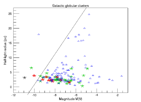
Figure 4: $R_{h}$ vs $M_{V}$ for 146 Galactic globular clusters. The Baumgardt’s set is marked by red asterisks; the CC set by green asterisks; the remaining clusters by blue triangles. The M31 globular cluster G1 is marked by a black asterisk, the measurement for its $R_{\rm h}$ is taken from Barmby et al. (2002). Above the slanted line the red asterisk marks $\omega$ Cen, the green asterisk M54.

In Fig. 4 we show $R_{\rm h}$, the radius that contains half of the cluster stars in projection, versus $M_{V}$, the integrated luminosity, for 146 Galactic GCs (Mackey and van den Bergh 2005). Core collapse GCs are marked by green asterisks, the Baumgaurdt’s list of GCs are shown as red asteristicks and the remaining GCs are shown as blue triangles. There is a sharp edge to the main distribution of the clusters, called the Shapley line (van den Bergh 2008), and only 4 clusters (all belonging to the SC class) lie above the line (3 galactic GC and G1 from M31). We see that our sample of clusters is concentrated in a small area of the plot and, as far as this distribution is concerned, there is no considerable difference between the Baumgardt set and CC set. It was noticed Gebhardt et al. (2005) that to the extent that a massive, bound cluster can be viewed as a ‘mini-bulge’, it may be that every dense stellar system (small or large) hosts a central black hole. It is possible that there may be some previously unrecognized connection between the formation and evolution of globular clusters and their central black holes. Loosely bound clusters are indeed susceptible to strong evolution Gnedin & Ostriker (1997), while compact clusters are significantly more stable.

It is not known how significantly the evolutionary effects may influence the formation of the cluster’s central BH, or the survival of a cluster with a central IMBH. In (Baumgardt et al., 2005) it was proposed on the basis of N-body simulations of realistic mutli-mass star clusters that central IMBH speeds up the dissolution of a star cluster, especially if a cluster is surrounded by a tidal field. This would rule out the presence of central IMBH in BD and OH population, though not in YH. However, one YH cluster with reported central black hole is a core-collapsed cluster M15 and core-collapsed clusters are also ruled out by Baumgardt et al. (2004). We intend to develop some criteria to select a set of clusters for our observational program. It is tempting to speculate that it is worth to look for IMBH in dense, compact and high luminosity, and may be old, clusters rather than diffuse and low luminosity ones. Clearly, there is a contradiction between some theoretical approaches (for ex., Baumgardt et al. (2004), Baumgardt et al. (2005)) and observational reports, which only stimulates more efforts to resolve the issue of the presence of IMBHs in different types of GCs.

3.2 Selection of Targets and Observational Strategy

Ideally, we would monitor all Galactic globular clusters. However, in practice it is a very difficult task. Even in our selected candidates list (Table 1) it is found that the optical depth varies considerably. Besides, the tentative results of Sec. 3.1 show that it might be useless to look for diffuse, faint and distant clusters. Moreover, in PCC clusters, if we take into account the mass segregation effect, and/or a mass distribution law more concentrated towards the centre, a $r^{-7/4}$ profile, the lensing rate increases. For example, for nearby 47 Tuc, NGC 6397, and NGC 6752 it would nearly double ($18.6\times 10^{-6}$, $7.9\times 10^{-6}$ and $2.6\times 10^{-6}$, respectively).

Assuming the threshold optical depth for choosing the observational targets as $1\times 10^{-6}$, we plot in Figure 5 the dependence of the optical depth on core radius and central density. In order to have larger optical depth, a cluster has to have either large core radius or/and large central density, though the optical depth rises faster with the central density rather than the core radius. According to Fig. 4 and section 3.1, dense compact clusters are potentially better targets for monitoring programs aimed at detecting IMBHs.

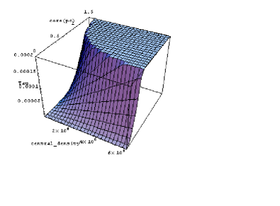
Figure 5: Dependence of optical depth (Tau) on central density and core radius

Our observational program suggests monitoring the cores (core radius) of selected globular clusters with the frequency of once a month in two filter-bands V and I using 2m class telescope. This particular choice of filters is to eliminate chromatic false events. The advantage of this proposed method is that it offers a direct relationship between the lens mass and the timescale of the ML event. In a typical ML event, only $t_{\rm E}$ can be measured directly and if the distance to the source is known, the remaining three physical parameters, lens mass $M_{\bullet}$, distance to the lens $D_{\rm L}$ and transverse velocity $v$, are in a degenerate combination,

$$t_{\rm E}[secs]=\frac{1.4}{v}\left(\frac{M_{\bullet}}{M_{\odot}}\right)^{1/2}\left(D_{\rm L}\left(1-\frac{D_{\rm L}}{D_{\rm S}}\right)\right)^{1/2},.$$ (18)

For example, in the Galactic ML events $D_{\rm L}$ is not known and $v$ can be anywhere in the range $0<v<600$ km/sec, resulting in a distribution of lens masses from $0.1\lesssim M_{\bullet}\lesssim 10\,M_{\odot}$ (Wambsganss, 2006). In a GC microlensing, no star not belonging to a cluster can be a source, thus even if the source is not directly detected, its tranverse velocity is within the range of cluster’s velocity dispersion (Sect. 2.2). The same is true for the distance to the source; distance to the lens is assumed to the cluster distance. Moreover, lens mass is constrained theoretically (Sect. 1.2) and source mass is constrained by the cluster mass function.

3.3 Prospects for Detection

The requirements of a traditional absolute photometry argue that cluster ML observations shall be carried with a large telescope with subarcsecond seeing Gyuk & Holder (1998). However, the cores of most GCs are not resolved even with an HST and, besides, it is not necessary to monitor every star in a globular cluster; the differential imaging analysis (DIA) takes the practice of crowded field photometry to its extreme limit. DIA is sensitive to ML events even when the source star is too faint to be detected at the baseline (Bond et al. 2001). We do not expect to be able to resolve the source star in the crowded centres of globular clusters, but with a careful application of DIA we do expect to be able to detect the star during any suitably bright outburst episode.

To address the question of detectability of microlensing events in our sample of IMBH globular clusters (Table 1), we again take the case of the cluster M15 as an example. M15 was observed for feasibility in April 2008. The observations were carried out on the 2-m Himalayan Chandra Telescope (HCT) of the Indian Institute of Astrophysics, equipped with a 2K$\times$2K CCD, in $V$ and $I$ bands.

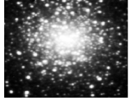
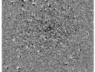
Figure 6: Top: $2\times 2$ arcmin central region of the globular cluster M15 in V-band (Image-1); Bottom: The difference between Image-1 and Image-2, made with the ISIS package.

In Fig. 6 (Top) we show the central $2\times 2$ arcmin square region of M15, observed in $V$-band for 50 seconds (Image-1). This exposure time was decided to avoid saturation of the core of the cluster in the images. In Fig. 6, Bottom we show a difference image between Image-1 and another image taken later in the same night (Image-2). The subtraction was done using the ISIS Differential Image Analysis package (Alard & Lupton, 1998). If a microlensing event of detectable amplitude occurs between these two exposure, we can see it appearing as a stellar image in the difference image (Fig. 6, Bottom. This is irrespective of whether the lensed star is resolved on not in the original image. However, this residual image may be (and is, indeed) affected by the imperfect substraction of bright stars. The histogram of the pixel values due to both resolved and unresolved stars is shown in the top panel of Fig. 7. In the bottom panel of Fig. 7, is shown the histogram of residual pixel values in this difference image. This distribution is nearly gaussian. The standard deviation of this residual pixel value distribution is 75 ADUs (1 ADU = 1.22 electrons).

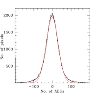
Figure 7: Top: A histogram of the pixel values due to both resolved and unresolved stars in Image-1; Bottom: A histogram of the pixel values in the difference image (Fig. 6 Bottom).The solid curve is the Gaussian fit to the distribution.

The total counts in any star-like image in this difference image are contained within a radius of at least 5 pixels (which is around 1.5 arcsecs for HCT). So the contribution of noise pixels in this region is $\sim 75\times\sqrt{3.14\times 5\times 5}\approx 665$ ADUs. To attain a S/N of $3$, the total counts within the stellar PSF have to be $\sim 1995$ ADUs. This would correspond to a limiting magnitude in V-band of 20.2, calculated using the following equation,

$$m=-2.5\log{(\mbox{count})}+2.5\log{(\mbox{Exp.time)}}+\mbox{Zero-point}\,,$$ (19)

where the zero-point for HCT in $V$-band is $24.25$ mag (D. K. Sahu, private communication). Thus, in this observational setup, we shall be able to detect a stellar source in the difference image to a magnitude limit of $m\approx 20.2$ in V-band. In Fig. 8 we show the HCT limiting magnitude for detection of stars in M15 undergoing microlensing for various amplication factors. We would like to mention that co-adding several 50 seconds exposures during one night reduces the noise, and thereby increases our detection limits.

Figure 8: HCT limiting magnitude for detection of stars in M15 undergoing lensing event versus lensing amplification.

It is interesting to mention that, inevitable in the case of a GC microlensing effects of blending (the contribution to the observed ML light curve from other unassociated sources) could be used to learn more about the lensing event than would be possible if there were no blending. The rate of lensing can actually increase in the crowded fields Di Stefano & Esin (1995), because there are many possible lensing events associated with the low-mass stars in the resolution cone of the telescope, instead of just one event associated with lensing of a single isolated star. For example, observing a region at $\mu_{V}=19^{\rm mag}/1\,{\rm arcsec}^{2}$ increases event probability by more than a factor of ten compared to observing in a 14.5 mag region (Colley, 1995). Blending plays a significant role in making the lensing of lowest mass stars either more or less observable. Blending also reduces the duration of events as well, thus it would reduce somewhat the rather long baseline of observations necessary for central BH cluster microlensing (Table 1).

3.4 Identifying genuine ML events

One major difficulty in identifying genuine lensing events is contamination by variable stars (periodic variables, cataclysmic variables (CVs) such as classical novae and dwarf novae (DN)). Globular clusters contain very few CVs and especially erupting CVs, which may mimic microlensing events (Della Valle & Livio 1996). The total number as of 2007 was 12 DN in 7 galactic globular clusters. The light curves of variable stars are much different from symmetric and achromatic Paczynski (1986) curves shown by lensing events. Most stellar variables are normally bluer when they are at maxmimum flux (Sterken & Jaschek 1996). Thus by carrying out two colour photometry in V and I bands, and by fitting the observed light curves to a Paczynski curve, variable stellar sources that may cause contamination can be removed. The estimated timescales of GC ML events are of the order of a year, whereas, most of the. variable stars in GCs have short periods ($<$ 100 days). Therefore, by analysing the observed candidate light curves for the abovementioned properties, contaminating stellar variables can be efficiently removed from genuine ML events.

Self-lensing events may present a challenge due to its higher event rate (Sec. 2.3). However, as far as competition between IMBH and self-lensing is concerned, the probabilities are very different. The probability of self-lensing does not depend as drastically on the radial distance as the IMBH lensing. If we consider a tube going through the GC centre and having, for example, a radius = core radius (which is much more than the radius of an IMBH influence), the ratio of self-lensing probabilities would roughly go as $\tau_{core}/\tau_{allcluster}\propto\frac{1}{2}r_{core}/r_{allcluster}$, which shows immediately how negligible it would be in the centre. Stars behind the cluster centre cannot contribute to self-lensing optical depth, any self-lensing event there would only contribute to the photometric noise. Also, contrary to the tentative conclusion on the choice of GC to look for IMBH lensing, the less centrally concentrated, loose and diffuse clusters are more favoured for self-lensing search, and such clusters are excluded from our current proposal. In adddition, self-lensing time scales are of the order of days (see Section 2.3), compared to the year-long time scales of GC ML events (see bottom panel of Fig. 3).

GC stars can also be affected by microlensing due to compact matter in the Milky Way not associated to a globular cluster (Gyuk & Holder, 1998; Rhoads & Malhotra, 1998). However, in such cases, the lens transverse velocity is set to that of the Galactic disk rotation, $v\approx 220$ km/sec, which would give the typical timescale of event $\sim 20-30$ days. Such events too will occupy a separate region on the amplitude-duration diagram and again can be easily distinguised from long duration ML events and eliminated.

4 Conclusion

Determining whether globular clusters contain IMBHs is a key problem in astronomy. They may contribute as much as $\Omega\approx 0.02$ to the cosmic baryon budget. Their cosmic mass density could exceed that of supermassive BHs ($\Omega\approx 10^{-5.7}$) and the observations do not even rule out that they may account for all the baryonic dark matter in the Universe ($\Omega\approx 10^{-1.7}$) van der Marel (2003). They also may have profound influence on the evolution and survival of globular clusters. In this paper, we have outlined the novel technique for using microlensing to detect IMBH in the centres of GCs. We suggest that dense and hight luminosity GCs are better suited to search for IMBH than diffuse and low luminosity GCs. The OH, BD and SC clusters are the most likely ones.

Our suggested monitoring programme of observing $\sim$100 clusters over a 10 year baseline with a time resolution of 1 observation per month will permit detection of one ML event. Such a monitoring programme is feasible on any dedicated 2m class telescope involved solely in monitoring astronomical sources. All the potential contaminants to this lensing signal (Section 3.4), can be easily identified and eliminated from the true ML events.

5 Acknowledgments

We thank the anonymous referee for his/her helpful comments. M. S. would like to thank Sohrab Rahvar with whom this project has started. Authors would also like to thank the Indian Institute of Astrophysics and especially our Observatories’ TACs for providing us with the opportunity to start the project.

Table 1: Globular cluster candidates for the central black hole; data and classifications

Cluster	Other	CC♣	$R_{\odot}$	$\sigma$	Core radius	$\log{\rho_{0}}$	$N_{\rm event}$	$\langle t_{\rm E}\rangle$	Class	Refs
name			$\rm Kpc$	$\rm km/s$	$\theta_{c}\,(r_{c}$, pc)	$M_{\odot}\,{\rm pc}^{-3}$	$10^{-6}$	days
NGC104	47 Tuc	c?	4.5	11.6	$23.1^{\prime\prime}$(0.6)	5.0	9.52	300	BD	3,4
NGC362		c?	8.6	6.4	$0.19^{\prime}$(0.52)	5.22	9.39	507	YH	4,8,9,10
NGC1851			12.1	11.3	′(0.25)	5.7	8.0	209	OH	8,10,11
NGC1904	M79	c?	13.0	5.2	$0.16^{\prime}$(0.66)	4.2	1.5	704	OH	4,8,10
NGC2808			9.6		$0.25^{\prime}$(0.73)	4.9	8.9	287	OH	8,10,11
NGC5139†	$\omega$ Cen		5.2	18.47	$2.4^{\prime}$(3.6)	7.748	3072.7	320	SC	10,20
NGC5272	M3	c?	10.4	4.8	$0.55^{\prime}$(1.26)	3.66	1.52	1053	YH	1,5,8,10,17
NGC5286			11.3	8.6	$0.29^{\prime}$(0.95)	4.3	3.8	510	OH	2,5,8,9
NGC5694			34.7	6.1	$0.06^{\prime}$(0.6)	4.3	1.51	572	OH	2,5,8,9
NGC5824♠		c?	32.0	11.1	$0.05^{\prime}$(0.20)	5.3	1.68	182	OH	2,5,8,9
NGC5904	M5		7.5	6.5	$0.42^{\prime}$(0.89)	4.0	1.66	654	OH	1,5,8
NGC5946		c	10.6	4.0	$0.08^{\prime}$(0.25)	4.8	0.83	563	OH	4,5,8
NGC6093	M80		10.0	14.5	$0.15^{\prime}$(0.44)	5.4	3.04	206	OH	2,5,8,9
NGC6205	M13		7.7	7.1	$0.78^{\prime}$(1.75)	3.4	1.6	839	OH	1,8
NGC6256	Ter12	c	8.4	6.6	$0.02^{\prime}$(0.05)	6.6	2.1	153	BD	4,8,11
NGC6266	M62	c?	6.9	15.4	$0.18^{\prime}$(0.36)	5.7	13.6	176	OH	1,2,5,8
NGC6284		c	15.3	6.8	$0.07^{\prime}$(0.312)	5.2	3.24	370	OH	4,5,8,9
NGC6293		c	8.8	8.6	$0.05^{\prime}$(0.128)	6.3	6.9	187	OH	4,5,8,9
NGC6325		c	8.0	6.4	$0.03^{\prime}$(0.07)	6.7	5.16	186	OH	4,5,8,9
NGC6333	M9	c	7.9	7.59	$0.58^{\prime}$(0.91)	4.087	2.13	566	OH	4,9,10
NGC6342		c	8.6	5.2	$0.05^{\prime}$(0.125)	5.4	0.82	306	BD	1,4,5,8
NGC6355		c	9.5	9.02	$0.05^{\prime}$(0.14)	4.429	0.11	187	OH	4,9,10
Ter 2	HP3	c	8.7	3.2	$0.03^{\prime}$(0.31)	4.261	0.4	784	BD	4,9,10
HP 1		c	14.1	6.35	$0.03^{\prime}$(0.58)	4.329	1.51	540	OH	4,9,10
Ter 1	HP2	c	5.6	2.04	$0.04^{\prime}$(0.3)	3.891	0.15	1209	YH	4,9,10
NGC6380	Ton1	c?	10.7	6.27	$0.34^{\prime}$(1.05)	4.64	10.2	736	BD	4,9,10
NGC6388			10.0	18.9	$0.12^{\prime}$(0.35)	5.7	73.5	337	BD	2,8,9
NGC6397♠		c	2.4	4.5	$0.05^{\prime}$(0.2)	5.68	4.02	448	OH	1,2,8,9,14
Ter 5			10.3	11.76	$0.18^{\prime}$(0.54)	6.38	146.9	282	BD	1,10
NGC6440			8.4	9.0	′(0.36)	5.63	11.6	300	BD	10,16,17
NGC6441			11.7	10.0	′(0.5)	5.57	19.5	319	BD	10,16,17
NGC6453		c	9.6	6.88	$0.07^{\prime}$(0.2)	4.504	0.27	293	OH	4,9,10
Ter 6	HP5	c	9.5	7.11	$0.05^{\prime}$(0.31)	4.977	1.9	353	BD	4,9,10
NGC6522		c	7.8	7.3	$0.05^{\prime}$(0.11)	6.1	3.2	205	OH	1,4,5,8
NGC6540♡	Djorg3	c?	3.7	6.0	$0.03^{\prime}$(0.03)	5.24	0.03	130	OH	1,2,8
NGC6541♠		c?	7.0	8.2	$0.3^{\prime}$(0.13)	5.5	1.2	198	OH	1,2,8
NGC6544		c?	2.7	9.07	$0.05^{\prime}$(0.04)	5.73	0.2	100	OH	1,4,9,10
NGC6558		c	7.4	3.5	$0.03^{\prime}$(0.07)	5.6	0.41	341	OH	4,5,8,9
NGC6626	M28		5.6	8.23	$0.24^{\prime}$(0.417)	4.9	2.9	354	OH	8,10,11
NGC6642		c?	8.4	3.86	$0.1^{\prime}$(0.244)	5.244	2.2	577	YH	4,9,10
NGC6656	M22		3.2	16.99	$1.42^{\prime}$(1.32)	4.0	3.67	305	OH	10,11,17,19
NGC6681	M70	c	9.2	10.0	$0.03^{\prime}$(0.08)	6.5	4.3	128	OH	1,4,8
NGC6715♠‡	M54		26.3	20.2	$0.11^{\prime}$(0.9)	6.3	339.4	212	SC	2,21
NGC6717	Pal9	c?	7.1	3.72	$0.08^{\prime}$(0.13)	5.134	0.5	437	OH	4,9,10
NGC6752		c	4.0	12.4	$0.17^{\prime}$(0.2)	5.2	1.33	163	OH	1,4,5,8
NGC7078	M15	c	10.3	14.1	$0.07^{\prime}$(0.2)	6.87	143	217	YH	1,4,7
NGC7099	M30	c	8.0	5.8	$0.06^{\prime}$(0.14)	5.9	3.3	291	OH	1,4,8
G1		c?	770	25.1	$0.21^{\prime\prime}$(0.78)	5.67	1080.9	673	SC	8,12,15

The data in this table is a compilation from various published datasets. Where it was possible, we chose the latest available references.

Footnotes to the Table 1:

$\clubsuit$ CC: c=post-core-collapse morphology; c?=possible p.c.c.

$\heartsuit$ The central density $\rho_{0}$ was calculated using the formula (Ref. 13)

$$\rho_{0}=\frac{3.44\times 10^{10}}{Pr_{c}}10^{-0.4\mu_{\rm V}(0)}\left(\frac{M}{L_{\rm V}}\right)\,M_{\odot}\,{\rm pc}^{-3}\,,$$

with $P\approx 2$ (Ref. 13) and $M/L_{\rm V}=1.1\pm 0.6$ (Ref. 18). The other values for this formula were taken from Ref. 10.

$\spadesuit$ Not likely to host a black hole, according to Ref. 2, belongs, however, to the CC set.

$\dagger$ Instead of $r_{c}$ radius of BH influence was used for calculations, see Sec. 2.4

$\ddagger$ The latest data is taken from Ibata et al. 2009

REFERENCES TO THE TABLE 1

1. P. C. Freire et al., 2005, ASP Conf. Ser. 328, eds. F. A. Rasio & I. H. Stairs
2. Baumgardt H., Makino J., & Hut P., 2005, ApJ , 620, 238.
3. P. C. Freire et al, 2001, MNRAS , 326, 901.
4. Trager S. C., King I. & Djorgovski S., 1995, AJ , 109, 218.
5. P. Dubath, G. Meylan and M. Mayor, 1997, A&A, 324, 505.
6. G. Meylan and M. Mayor, 1986, A&A, 166, 122.
7. De Paolis F., Ingrosso G., & Jetzer Ph., 1996, ApJ , 470, 493.
8. C. Pryor and G. Meylan, 1993, in Structure and Dynamics of Globular Clusters, eds. S. Djorgovski, G. Meylan, ASP Conf. Series 50, p. 357.
9. Harris Catalogue (Harris, W.E., 1996, AJ, 112, 1487);
(http://physwww.mcmaster.ca/ %7Eharris/mwgc.dat)
10. Webbink R. F., 1985, Proc. IAU Symp. 113, Dynamics of Star Clusters, eds. Goodman J. & Hut P., (Kluwer, Dordrecht) p. 541.
11. S. Djorgovski, 1993, in Structure and Dynamics of Globular Clusters, eds. Djorgovski S, & Meylan G. ASP Conf. Series, 50, p. 373 12. J. Ma, et al. 2007, MNRAS , 376:1621
13. S. S. Larsen, 2001, AJ, 122, 1782
14. E. Dalessandro, B. Lanzoni, F. R. Ferraro, R. T. Rood, A. Milone, G. Piotto & E. Valenti, 2007, ArXiv e-prints, 712, arXiv:0712.4272.
15. G. Meylan, et al. 2001, AJ , 122:830.
16. L. Origlia, E. Valenti & R. M. Rich, 2008, MNRAS , 388, 1419.
17. D. E. McLaughlin & R. P. van der Marel, 2005, ApJS, 161:304.
18. P. Côté, 1999, AJ , 118, 406.
19. C. Ding, C. Li & W. Jia-Ji, Chin. Phys. Lett.,2004, 21(8).
20. Anderson, J., & van der Marel, R. P. 2009, arXiv:0905.0627; Noyola, E., Gebhardt, K., & Bergmann, M. 2008, ApJ , 676, 1008.
21. Ibata, R., et al. 2009, ApJL , 699, L169

References

- Anderson & James (2009) Anderson, J. P., & James, P. A. 2009, arXiv:0907.0034
- Alcock et al. (1997) Alcock, C., et al. 1997, ApJ , 479, 119
- Alard & Lupton (1998) Alard, C., & Lupton, R. H. 1998, ApJ , 503, 325
- Bahcall & Ostriker (1975) Bahcall, J. N., & Ostriker, J. P. 1975, Nature , 256, 23
- Barmby et al. (2002) Barmby, P., Holland, S., & Huchra, J. P. 2002, AJ , 123, 1937
- Barth et al. (2004) Barth, A., Ho, L., & Sargent, W. 2004, AGN Physics with the Sloan Digital Sky Survey, 311, 91
- Baumgardt et al. (2003a) Baumgardt, H., Hut, P., Makino, J., McMillan, S., & Portegies Zwart, S. 2003a, ApJL , 582, L21
- Baumgardt et al. (2003b) Baumgardt, H., Makino, J., Hut, P., McMillan, S., & Portegies Zwart, S. 2003b, ApJL , 589, L25
- Baumgardt et al. (2004) Baumgardt, H., Portegies Zwart, S. F., McMillan, S. L. W., Makino, J., & Ebisuzaki, T. 2004, The Formation and Evolution of Massive Young Star Clusters, 322, 459
- Baumgardt et al. (2005) Baumgardt, H., Makino, J., & Hut, P. 2005, ApJ , 620, 238
- Binney & Tremaine (1987) Binney J. and Tremaine S. 1987, The Galactic Dynamics (Princeton: Princeton University Press)
- Bond et al. (2001) Bond, I. A., et al. 2001, MNRAS , 327, 868
- Brown & Bethe (1994) Brown, G. E., & Bethe, H. A. 1994, ApJ , 423, 659
- Chernoff & Djorgovski (1989) Chernoff D. F. and Djorgovski S., 1989, ApJ , 339, 904
- Colley (1995) Colley W. N., 1995, AJ , 109, 440
- Della Valle & Livio (1996) Della Valle M. & Livio M., 1996, ApJL , 457, L77
- De Rijcke et al. (2006) De Rijcke S., Buyle P. & Dejonghe H., 2006, MNRAS , Letters 368 (1), L43-L46
- De Paolis et al. (1996) De Paolis F., Gurzadyan V. G. & Ingrosso G., 1996, A&A, 315, 396
- Devecchi et al. (2007) Devecchi B., Colpi M., Mapelli M. & Possenti A., 2007, MNRAS , 380, 691
- Di Stefano & Esin (1995) Di Stefano, R., & Esin, A. A. 1995, ApJL , 448, L1
- Djorgovski & King (1986) Djorgovski S., and King I., 1986, ApJ , 305, 61
- Ferraro et al. (2003) Ferraro F. R., Possenti A., Sabbi E., Laggani P., Rood R. T., D’Amigo N. and Origlia N., 2003, ApJ , 595, 179
- Filippenko & Ho (2003) Filippenko, A. V., & Ho, L. C. 2003, ApJL , 588, L13
- Frank & Rees (1976) Frank, J. & Rees M. J., 1976, MNRAS , 176, 633
- Gebhardt et al. (2000) Gebhardt K., et al. 2000, ApJ , 539, L13
- Gebhardt et al. (2005) Gebhardt, K., Rich, R. M., & Ho, L. C. 2005, ApJ , 634, 1093
- Gerssen et al. (2002) Gerssen J., van der Marel, R. P. Gerbhardt K., Guhathukurta, P., Peterson R. C., and Pryor C., 2002, AJ , 124, 3270
- Gerssen et al. (2003) Gerssen J., van der Marel, R. P. Gerbhardt K., Guhathukurta, P., Peterson R. C., and Pryor C., 2003, AJ , 125, 376
- Gnedin & Ostriker (1997) Gnedin O. Y. and Ostriker J. P., 1997, MNRAS , 323, 529
- Gultekin et al. (2009) Gultekin K. et al. 2009, ApJ , 698, 198
- Gyuk & Holder (1998) Gyuk, G., & Holder, G. P. 1998, MNRAS , 297, L44
- Harris (1996) Harris Catalogue (Harris, W.E., 1996, AJ, 112, 1487); (http://physwww.mcmaster.ca/%7Eharris/mwgc.dat)
- Heggie et al. (2007) Heggie, D. C., Hut, P., Mineshige, S., Makino, J., & Baumgardt, H. 2007, PASJ, 59, L11
- Hurley J.R. (2007) Hurley J. R., 2007, MNRAS , 379, 93
- Kawakatu & Umemura (2005) Kawakatu N., Umemura M. , 2005, ApJ, 628, 721
- Kiselev et al. (2008) Kiselev A. A., et al., 2008, Astronomy Letters, 34, 529
- Kormendy & Richstone (1995) Kormendy J. and Richstone D., 1995, AJ , 33, 581.
- Lanzoni et al. (2007) Lanzoni, B., Dalessandro, E., Ferraro, F. R., Miocchi, P., Valenti, E., & Rood, R. T. 2007, ApJL , 668, L139
- Lugger et al. (1987) Lugger P. M., Cohn H., Grindlay J. E., Baylin C.D. and Hertz P., 1987, ApJ , 320, 482
- Maccarone et al. (2005) Maccarone T. J., R. P. Fender and A. K. Tzioumis, 2005, MNRAS , 365, L17
- Mackey & van den Bergh (2005) Mackey A. D. and van den Bergh S., 2005, MNRAS , 360, 631
- Madau & Rees (2001) Madau P. and Rees M. J., 2001, ApJ , 551, L27
- Magorrian et al. (1998) Magorrian J. et al. 1998, AJ , 115, 2285
- McLaughlin et al. (2006) McLaughlin D. E., Anderson J., Meylan G., Gebhardt K., Pryor C., Minniti D., Phinney S. 2006, ApJS , 166, 249
- Miller & Hamilton (2002) Miller M. C. and Hamilton D. P., MNRAS , 2002, 330, 232
- Miocchi (2007) Miocchi, P. 2007, MNRAS , 381, 103
- Noyola & Gebhardt (2006) Noyola, E. & Gebhardt, K. 2006, AJ , 132, 447
- Noyola et al. (2008) Noyola, E., Gebhardt, K., & Bergmann, M. 2008, ApJ , 676, 1008
- Paczynski (1994) Paczynski, B. 1994, Acta Astronomica, 44, 235
- Paczynski (1986) Paczynski, B. 1986, ApJL , 304, L1
- Pooley & Rappaport (2006) Pooley, D., & Rappaport, S. 2006, ApJL , 644, L45