Determination of Rate Constant of Chemical Reactions by Simple Numerical Nonlinear Analysis

Abstract

For some centuries, first order chemical rate constants were determined mainly by a linear logarithmic plot of reagent concentration terms against time where the initial concentration was required, which is experimentally often a challenging task to derive accurate estimates. By definition, the rate constant was deemed to be invariant and the kinetic equations were developed with this assumption. A reason for these developments was the ease in which linear graphs could be plotted. Here, different methods are discussed that does not require exact knowledge of initial concentrations and which require elementary nonlinear analysis and the ensuing results are compared with those derived from the standard methodology from an actual chemical reaction, with its experimental determination of the initial concentration with a degree of uncertain. We verify experimentally our previous theoretical conclusion based on simulation data [ J. Math . Chem 43 (2008) 976–1023] that the so called rate constant is never constant even for elementary reactions and that all the rate laws and experimental determinations to date are actually averaged quantities over the reaction pathway. We conclude that nonlinear methods in conjunction with experiments could in the future play a crucial role in extracting information of various kinetic parameters.

Keywords: [1] elementary reaction rate constant , [2] activity and reactivity coefficients, [3] elementary and ionic reactions without pre-equilibrium.
AMS Classification: 80A10, 80A30, 81T80, 82B05, 92C45, 92E10, 92E20.

1 1. INTRODUCTION AND METHODS

As alluded in the abstract, most kinetic determinations use logarithmic plots with known initial concentrations, although there have been attempts [1, 2, and refs. therein]. (There are possible ambiguities in [1] concerning choice of variables that will not be discussed.) However all these publications hitherto assume constancy of the rate constant $k$ and do not focus on nonlinear analysis (NLA), as will be attempted here in preliminary form. We analyze kinetic data of the tert butyl chloride hydrolysis reaction in ethanol solvent (80%v/v) derived from the Year III teaching laboratory of this University (UM); 0.3mL of the reactant was dissolved in 50mL of ethanol initially. The reaction was conducted at $30^{o}C$ and monitored over time (minutes) by measuring conductivity ($\mu\text{S cm}^{-1}$) due to the release of $\text{H}^{+}$ and $\text{Cl}^{-}$ ions as shown below (1),

$$\mbox{C${}_{4}$H${}_{9}$Cl}+\mbox{H${}_{2}$O}\,\,\stackrel{{\scriptstyle k}}{{\longrightarrow}}\,\,\mbox{C${}_{4}$H${}_{9}$OH}+\mbox{H}^{+}+\mbox{Cl}^{-}$$ (1)

and $\lambda_{\infty}=2050\mu\text{S cm}^{-1}$ was determined by heating the reaction vessel at the end of the monitoring to $60^{o}$C until there was no apparent change in the conductivity when equilibrated back at $30^{o}$C. “Units” in the figures and text refers to $\mu\text{S cm}^{-1}$. It would be inferred here that either because of evaporation or the temperatures not equilibrating after heating, the measured $\lambda_{\infty}$ is larger than the actual one. Linear proportionality is assumed in $\lambda$ and the extent of reaction $x$, where the first order law (c being the instantaneous concentration and $a$ the initial concentration) is $\frac{dc}{dt}=-kc=-k(a-x)$; with $\lambda_{\infty}=\alpha a,\lambda_{t}=\alpha x$ and $\lambda(0)=\lambda_{0}=\alpha x_{0}$, integration yields for assumed constant $k$

$$\ln\frac{(\lambda_{\infty}-\lambda_{0})}{(\lambda_{\infty}-\lambda(t))}=kt$$ (2)

Eqn.(2) determines $k$ if $\lambda_{0}$ and $\lambda_{\infty}$ are known.

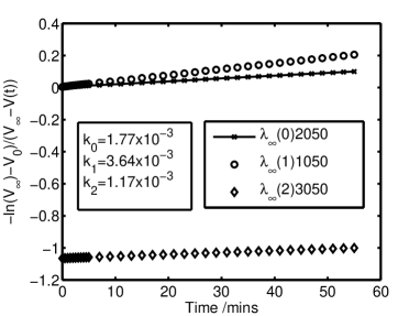
Figure 1: Integrated equation(2) plot with $\lambda_{\infty}$ from experiment (0) and from two different arbitrary values (1,2) for $\lambda_{\infty}$

The plot of (2) was made for the same experimental values with different $\lambda_{\infty}$’s, both higher and lower than the experimental value. We find that the rate constant for the NLA was higher, leading to a lower value of $\lambda_{\infty}$ which is consonant with evaporation of solvent or the non-equilibration of temperature prior to measurement to determine $\lambda_{\infty}$.Except for the last subsection, we shall do a NLA based on constant $k$ assumption.

1.1 1.1 Method 1

Under linearity argument and constant $k$, the rate equation $\frac{dc}{dt}=-kc=-k(a-x)$ reduces to

$$\frac{\lambda(t)}{dt}=-k\lambda(t)+\lambda_{\infty}.k$$ (3)

Hence a plot of $\frac{\lambda(t)}{dt}$ vs $t$ would be linear. We find this to be the case for polynomial order $npoly\leq 3$ as in Fig.(2) below for all data values; higher polynomial orders can be used in selected data points of the curve below, especially in the central region. Thus criteria must be set up to determine the appropriate regime of datapoints in the NLA.

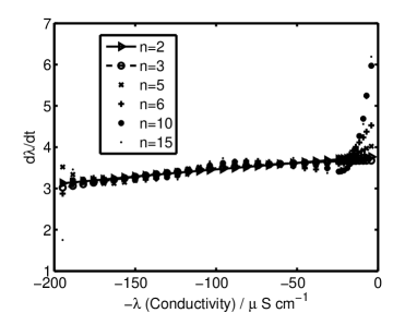
Figure 2: Method 1 graph showing linearity lower order polynomial fits

1.2 1.2 Method 2

Let $\alpha^{\prime}=\lambda_{\infty}-\lambda_{0}$, then $\ln\alpha^{\prime}-\ln(\lambda_{\infty}-\lambda)=kt$, then noting this and differentiating yields

$$\underbrace{\ln\left(\frac{d\lambda}{dt}\right)}_{Y}=\underbrace{-kt}_{Mt}+\underbrace{\ln[k(\lambda_{\infty}-\lambda_{0})]}_{C}$$ (4)

A typical plot that can extract $k$ as a linear plot of $\ln(d\lambda/dt)$ vs $t$ is given in Fig.(3). Linearity is observed for $npoly=2$ and smooth curves without oscillations for at least $npoly\leq 3$.

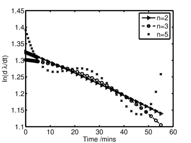
Figure 3: Method 2 where smooth curves are obtained for at least $npoly<4$

1.3 1.3 Other methods and considerations

A variant method similar to the Guggenheim method [2] of elimination is given below but where gradients to the conductivity curve is required, and where the average over all pairs is required.

$$\left\langle k\right\rangle=\frac{-2}{N(N-1)}\sum_{i}^{N}\sum_{j>i}^{N}\ln\left(\lambda^{\prime}(t_{i})/\lambda^{\prime}(t_{j})\right)/(t_{i}-t_{j})$$ (5)

It was discovered that the normal least squares polynomial method using Gaussian elimination [4, Sec.6.2.4,p.318 ]to derive the coefficients of the polynomial was highly unstable for $npoly>4$ and so for this work, we used a variant of the Orthogonal method modified for determination of differentials. The normal method defines the nth order polynomial $p_{n}(t)$ which is then expressed as a sum of square terms over the domain of measurement to yield $Q$ in eqns(6).

$$\begin{array}[]{rcl}p_{n}(t)&=&\sum_{j=0}^{n}h_{i}t^{j}\\ Q(f,p_{n})&=&\sum_{i=1}^{N}\left[f_{i}-p_{n}(t_{i})\right]^{2}\end{array}$$ (6)

The $Q$ function is minimized over the polynomial coefficient space. In the Orthogonal method adopted here, we express our polynomial expression $p_{m}(t)$ linearly in coefficients $a_{j}$ of $\varphi_{j}$ functions that are orthogonal with respect to an inner product definition. For arbitrary functions $f,g$, the inner product $(f,g)$ is defined below, together with properties of the $\varphi_{j}$ orthogonal polynomials.

$$\begin{array}[]{rcl}(f,g)&=&\sum_{k=1}^{N}f(t_{k}).g(t_{k})\\ (\varphi_{i},\varphi_{j})=0&(i\neq j);&\,\,\mbox{and}\,\,(\varphi_{i},\varphi_{i})\neq 0.\end{array}$$ (7)

$$\begin{array}[]{rll}\varphi_{i}(t)&=&(t-b_{i})\varphi_{i-1}(t)-c_{i}\varphi_{i-2}(t)\,(i\geq 1)\\ \varphi_{0}(t)&=&1,\mbox{and}\,\,\varphi_{j}=0\,\,\,j<1,\\ b_{i}&=&(t\varphi_{i-1},\varphi_{i-1})/(\varphi_{i-1},\varphi_{i-1})\,\,(i\geq 1)\\ c_{i}&=&(t\varphi_{i-1},\varphi_{i-2})/(\varphi_{i-2},\varphi_{i-2})\,\,(i\geq 2),c_{i}=0.\end{array}$$ (8)

We define the $m^{th}$ order polynomial and associated $a_{j}$ coefficients as:

$$\begin{array}[]{rll}p_{m}(t)&=&\sum_{j=0}^{m}a_{j}\varphi_{j}(t)\\[14.22636pt] a_{j}&=&(f,\varphi_{j})/(\varphi_{j},\varphi_{j}),(j=0,1,\ldots m)\\ \end{array}$$ (9)

The recursive definitions for the first and second derivatives are given respectively as:

$$\begin{array}[]{rll}\varphi^{\prime}_{i}(t)&=&\varphi^{\prime}_{i-1}(t)(t-b_{i})+\varphi_{i-1}(t)-c_{i}\varphi^{\prime}_{i-2}(t)\,(i\geq 1)\\ \varphi^{\prime\prime}_{i}(t)&=&\varphi^{\prime\prime}_{i-1}(t)(t-b_{i})+2\varphi_{i-1}^{\prime}(t)-c_{i}\varphi^{\prime\prime}_{i-2}(t)\,(i\geq 2)\end{array}$$ (10)

Here the codes were developed in C/C++ which provides for recursive functions which we exploited for the evaluation of all the terms. The experimental data were fitted to an $m^{th}$ order expression $\lambda_{m}(t)$ defined below

$$\lambda_{m}(t)=\sum_{j=0}^{n}h_{i}t^{j}\\$$ (11)

Figure(4)are plots for the different polynomial orders n. The orthogonal polynomial method is stable and the mean square error decreases with higher polynomial order (for the 36 data points) monotonically, but the differentials are not so stable, as shown in the previous figures.

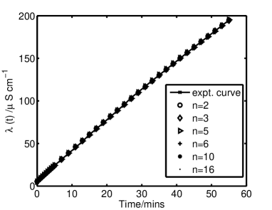
Figure 4: Plot using orthogonal polynomials for various orders $n$

Differentiating (4) for constant $k$ leads to (12) expressed in two ways

$$\frac{d^{2}\lambda}{dt^{2}}=-k\left(\frac{d\lambda}{dt}\right)\,(a)\,\mbox{or}\,k=-\frac{d^{2}\lambda}{dt^{2}}/\left(\frac{d\lambda}{dt}\right)\,(b)$$ (12)

Eq.(12(b)) suggests another way of computing $k$ for “well-behaved” values of the differentials, meaning regions where $k$ would appear to be a reasonable constant. The (a) form suggests an exponential solution. Define $\frac{d\lambda}{dt}\equiv dl$ and $\frac{d^{2}\lambda}{dt^{2}}\equiv d2l$. Then $dl(t)=A\exp(-kt)$ and $dl(0)=A=h_{2}$ from (11).Furthermore, as $t\rightarrow 0$, $k=\left(-2h_{2}/h_{1}\right)$ and a global definition of the rate constant becomes possible based on the total system $\lambda(t)$ curve.

With a slight change of notation, we now define $dl$ and $d2l$ as referring to the continuous functions $dl(t)=A\exp(-kt)$ and $d2l(t)=-kA\exp(-kt)$ and we consider $(d\lambda/dt)$ and $d^{2}\lambda/dt^{2}$ to belong to the values (11) derived from ls fitting where $(d\lambda/dt)=\lambda_{m}^{\prime}$,    $(d^{2}\lambda/dt^{2})=\lambda_{m}^{\prime\prime}$ which are the experimental values for a curve fit of order $m$. From the experimentally derived gradients and differentials, we can define two non-negative functions $R_{a}(k)$ and $R_{b}(k)$ as below:

$$\begin{array}[]{rll}R_{a}(k)&=&\sum^{N}_{i=1}\left(\frac{d^{2}\lambda(t_{i})}{dt^{2}}+kdl(t_{i})\right)^{2}\\[8.5359pt] R_{b}(k)&=&\sum^{N}_{i=1}\left(\frac{d\lambda(t_{i})}{dt}-dl(t_{i})\right)^{2}\\ &\mbox{where}&\\ f_{a}(k)=R^{\prime}_{a}(k)&\mbox{and}&f_{b}(k)=R^{\prime}_{b}(k)\end{array}$$ (13)

and a minimum exists at $f_{a}(k)=f_{b}(k)=0.$ We solve the equations $f_{a}$ , $f_{b}$ for their roots in k using the Newton-Raphson method and compute the rate constant $k$. The error threshold in the Newton-Raphson method was set at $\epsilon=1.0\times 10^{-7}$ We provide a series of data of the form $\left[n,A,k_{a},k_{b},\lambda_{a,\infty},\lambda_{b,\infty}\right]$ where $n$ refers to the polynomial degree, $A$ the initial value constant as above, $k_{a}$ and $k_{b}$ is the rate constant for function $f_{a}$ and $f_{b}$ (solved when the functions are zero respectively ) and likewise for $\lambda_{a,\infty}$ and $\lambda_{b,\infty}$. The $e$ symbol refers to base $10$ (decimal) exponents. The $\lambda_{\infty}$ values are averaged over all the (36) data points from the equation

$$\lambda_{\infty}=\frac{d\lambda(t)}{dt}\frac{1}{k}+\lambda(t)$$ (14)

The results are as follows:
$\left[2,3.7634e0,3.2876e-3,3.2967e-3,1.1506e3,1.1477e3\right]$,
$\left[3,3.6745e0,2.7537e-3,2.7849e-3,1.34756e3,1.3334e3\right]$,
$\left[4,3.6380e0,2.0973e-3,2.4716e-3,1.7408e3,1.4900e3\right]$,
$\left[5,4.0210e0,9.7622e-3,4.9932e-3,4.4709e2,7.9328e2,\right]$,
$\left[6,4.5260e0,4.1270e-2,8.9257e-3,1.7101e2,4.8403e2\right]$.
We noticed as in the previous cases that the most linear values occur for $1<n<4$. In this approach, we can use the $f_{a}$ and $f_{b}$ function similarity of solution for $k$ to determine the appropriate regime for a reasonable solution. Here, we notice a sudden departure of similar value between $k_{a}$ and $k_{b}$ (about 0.4 difference ) at $n=4$ and so we conclude that the probable “rate constant” is about the range given by the values spanning $n=2$ and $n=3$. Interestingly, the $\lambda_{\infty}$ values are approximately similar to the ones for method 1 and 2 for polynomial evaluation 2 and 3 for those methods. More study with reliable data needs to be done in order to discern and select appropriate criteria that can be applied to these non-linear methods.

1.4 1.4 Evidence of varying kinetic coefficient $k$

Finally, what of direct methods that do not assume the constancy of $k$ which was the case in the above subsections? Under the linearity assumption $x=\alpha\lambda(t)$, the rate law has the form $dc/dt=-k(t)(a-x)$ where $k(t)$ is the instantaneous rate constant and this form implies

$$k(t)=\frac{d\lambda/dt}{\lambda_{\infty}-\lambda(t)}$$ (15)

If $\lambda_{\infty}$ is known from accurate experiments or from our computed estimates, then $k(t)$ is determined; the variation of $k(t)$ provides crucial information concerning reaction kinetic mechanism and energetics, from at least one theory recently developed for elementary reactions [3] and for such theories and developments, it may be anticipated that nonlinear methods would be used to accurately determine $k(t)$ that would yield the so-called “reactivity coefficients” [3] that account for variations in $k$ that would provide fundamental information concerning activation and free energy changes.

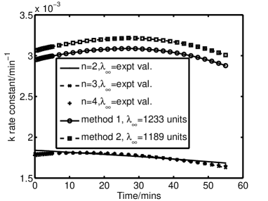
Figure 5: Variation of $k$ with time or concentration changes based on the experimental value $\lambda_{\infty}=2050\text{units}$ and the computations based on different polynomial degrees $n=2,3,4$ and the computed $\lambda_{\infty}$ values for Method 1 and Method 2 for fixed polynomial degree $n=3$.

Figure(5) refers to the computations under the assumption of first order linearity of concentration and the conductivity. Whilst very preliminary, non-constancy of the rate constants are evident, and one can therefore expect that another area of fruitful experimental and theoretical development can be expected from these results.

2 2. CONCLUSIONS

The results presented here provides alternative developments based on NLA that is able to probe into the finer details of kinetic phenomena than what the standard representations allow for, especially in the the areas of changes of the rate constant with the reaction environment. Such studies would involve building up another set of axioms that is consistent with a varying $k(t)$ kinetic coefficient. Even with the assumption of invariance of $k$, one can always choose the best type of polynomial order that is consistent with the assumption, and it appears that the initial concentration as well as the rate constant seems be be predicted as global properties based on the polynomial expansion.

3 ACKNOWLEDGMENTS

This work was supported by Science Faculty conference allocation and grants UMRG(RG077/09AFR), FRGS(FP037/2008C) and PJP(FP037/2007C) of the Malaysian Government.

References

- [1] P. Moore, Analysis of kinetic data for a first-order reaction with unknown initial and final readings by the method of non-linear least squares, J. Chem. Soc., Faraday Trans. I 68 (1972), 1890–1893.
- [2] E. A. Guggenheim, On the determination of the velocity constant of a unimolecular reaction, Philos Mag J Sci 2 (1926) 538–543 .
- [3] C. G. Jesudason, The form of the rate constant for elementary reactions at equilibrium from MD: framework and proposals for thermokinetics, J. Math . Chem 43 (2008) 976–1023.
- [4] S. Yakowitz and F. Szidarovsky,An Introduction to Numerical Computations, Maxwell Macmillan, New York, 1990