Rank-dependent deactivation in network evolution

Abstract

A rank-dependent deactivation mechanism is introduced to network evolution. The growth dynamics of the network is based on a finite memory of individuals, which is implemented by deactivating one site at each time step. The model shows striking features of a wide range of real-world networks: power-law degree distribution, high clustering coefficient, and disassortative degree correlation.

Since 1998, with the small-world model introduced by Watts and Strogatz WS98 , we have witnessed the emergence of a new science of networks, which has powerful function of describing structures AB02 ; CRTB07 and dynamics BLMCH06 ; DGM08 of many real systems. A network is a mathematical object which consists of vertices connected by edges. Despite differences in their nature, most real-world networks are characterized by similar topological properties, in contrast to those obtained by traditional random graphs. For instance, real networks display higher clustering than that expected from random networks ASBS00 . Also, it has been found that many large networks are scale free (SF) BA99 , which means a power-law distribution of connectivity, $P(k)\sim k^{-\gamma}$, where $P(k)$ is the probability that a vertex in the network is of degree $k$ and $\gamma$ is a positive real number determined by the given network. In order to understand how SF networks arise, Barabási and Albert (BA) proposed an evolving network model in 1999, which grows at a constant rate and new vertices attach to old ones with probability $\Pi(k)\sim k$ BA99 . In this way, vertices of high degree are more likely to receive further edges from newcomers.

For most networks, however, aging of sites usually occurs. For instance, in reference networks old papers are rarely cited; in social networks people of the same age are more likely to be friends. To study the effect of aging on network evolution, the BA model has been modified by incorporating time dependence in the network DM00 ; ZWZ03 ; HS04 ; HAB07 ; RL07 ; DKM08 ; CM09 . Dorogovtsev and Mendes studied the case when the connection probability of the new site with an old one is not only proportional to the degree $k$ but also to the power of its present age $\tau^{-\alpha}$ DM00 . They showed both numerically and analytically that the scale-free nature disappears when $\alpha<-1$. As an alternative, Zhu et al introduced the exponential decay function $e^{-\beta\tau}$ of its present age to the BA attachment probability ZWZ03 . It was found that the produced network is significantly transformed besides the change in the degree distribution. On the other hand, Klemm and Eguíluz KE02a observed the negative correlation between the vertex age and its rate of acquiring links from the network of scientific citations. Based on that, they investigated the finite collective memory of popular individuals and proposed a highly clustered scale-free network model KE02a ; KE02b . The model accounts for three empirical features: preferential attachment, power-law degree distribution, and negative correlation between age and connection rate.

Recently, Fortunato et al proposed a criterion of network growth that explicitly relies on the ranking of vertices FFM06 , which originates from the idea that the absolute importance (popularity or fitness) of an object is often difficult or impossible for strangers to measure in social networks. Instead, it is quite common to have a clear knowledge about the relative values of two objects, i.e., who is more popular or richer between two individuals. The rank-driven mechanism generates networks with the scale-free degree distribution when the probability to link a target vertex is any power-law function of its rank, even when one has only partial information of vertex ranks FFM06 ; TS07 . Since the perception of how items are ranked requires far less information than their actual importance, the rank-driven mechanism can well mimic the reality in many cases that the relative values of agents are easier to access than their absolute values. In this paper, we integrate rank with deactivation and study their influences on network evolution. Simulations show that interesting statistical properties of the generated network display good features observed in realistic systems.

The present model is based on the rank-dependent deactivating of vertices, which describes the growth dynamics of a network with directed links, run as follows. First, start from an initial network of $m$ completely connected seeds, whose states are active. By $k^{\text{in}}$ we denote the in-degree of the vertex, i.e., the number of edges pointing to the vertex. At each time step, add a new vertex $n$ with $m$ outgoing edges. The new vertex is disconnected at first, so $k_{n}^{\text{in}}=0$ at this point. Each vertex $i$ of the $m$ active vertices receives exactly one incoming edge, thereby $k_{i}^{\text{in}}\rightarrow k_{i}^{\text{in}}+1$. Then activate the new vertex $n$ and deactivate one (denoted by $j$) of the $m+1$ active vertices with probability

$$\Pi(j)=\frac{\gamma}{a+R_{j}},$$ (1)

where $a\geq 0$ is a constant bias and $\gamma$ is the normalization factor. $R_{j}\in[1,m+1]$ is the rank of $j$ among the $m+1$ active vertices. The average connectivity of the network is given by the number $m$ of outgoing edges per vertex. The new added vertex is always in the active state first and receives edges from subsequently added vertices until it is deactivated. Note that the larger rank a vertex possesses, the more difficult for it to be deactivated. For the case of the citation network, Eq. (1) means that the famous paper cited mostly is less possibility to be forgotten. In Ref. FFM06 , the model grows according to the rank-based preferential attachment $\Pi(n\rightarrow i)\sim R_{i}^{-\alpha}$. In case vertices are sorted by age $R(t)=t$, the older the vertex is, the higher possibility for it gaining new edges, coinciding with ours.

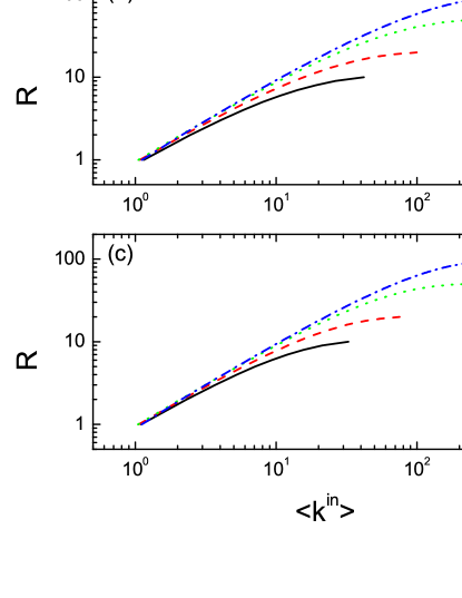
Figure 1: (Color online) Illustration of average $R$ versus average $k^{\text{in}}$ of the generated networks for various values of $m$: $m=10$ (solid line), $20$ (dashed line), $50$ (dotted line), and $100$ (dashed dotted line), respectively. The size of the network is $N=10^{5}$.

The choice of prestige measure can be arbitrary, either topological measures or physical ones. In present work we sort vertices by age for simplicity. Namely, the older the vertex is, the larger rank it possesses. Supposing the distribution of the in-degree of active vertices at time $t$ denoted by $p(k^{\text{in}},t)$, then we can write out the master equation

$$p(k^{\text{in}}+1,t+1)=[1-\Pi(k^{\text{in}})]p(k^{\text{in}},t),$$ (2)

where $\Pi(k^{\text{in}})$ is the deactivation probability of a vertex with in-degree $k^{\text{in}}$. To do further calculation, we should get the relation between $R$ and $k^{\text{in}}$. In Fig. 1 we plot $R$ as a function of $k^{\text{in}}$ of the model by numerical simulations. In order to reduce statistical error, the in-degrees of the vertices are calculated as an average. As it can be seen, there is a rough power law between $R$ and $k^{\text{in}}$, $R\sim\mu(k^{\text{in}})^{\nu}$ Note1 . Then one easily obtains $\Pi(k^{\text{in}})\sim\mu\nu(k^{\text{in}})^{\nu-1}\Pi(R)$, where $\Pi(R)$ is the deactivation probability of a vertex with rank $R$. Substituting them into Eq. (2), we get

$$p(k^{\text{in}}+1,t+1) = [1-\mu\nu(k^{\text{in}})^{\nu-1}\Pi(R)]p(k^{\text{in}},t)$$ (3)

$$= \left[1-\frac{\gamma\mu\nu(k^{\text{in}})^{\nu-1}}{a+\mu(k^{\text{in}})^{\nu}}\right]p(k^{\text{in}},t).$$

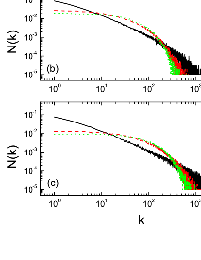
Figure 2: (Color online) Log-log plots of the vertex degree distribution of the generated networks for different values of $a$: $a=0$ (solid line), $m$ (dashed line), and $N$ (dotted line), respectively. All the experiment networks have a total number of vertices $N=10^{5}$.

The subsequent thing is just to follow the analytical method in Ref. KE02a . Imposing the stationarity condition $p(k^{\text{in}},t+1)=p(k^{\text{in}},t)$ yields

$$p(k^{\text{in}}+1)-p(k^{\text{in}})=-\frac{\gamma\mu\nu(k^{\text{in}})^{\nu-1}}{a+\mu(k^{\text{in}})^{\nu}}p(k^{\text{in}}).$$ (4)

Assuming $k^{\text{in}}$ changes continuously, we have

$$\frac{dp(k^{\text{in}})}{dk^{\text{in}}}=-\frac{\gamma\mu\nu(k^{\text{in}})^{\nu-1}}{a+\mu(k^{\text{in}})^{\nu}}p(k^{\text{in}}),$$ (5)

and accordingly obtain the solution

$$p(k^{\text{in}})=b[a+\mu(k^{\text{in}})^{\nu}]^{-\gamma},$$ (6)

with the appropriate normalization constant $b$. In case the total number $N$ of vertices in the network is large compared with the number $m$ of active vertices, the overall in-degree distribution $N(k^{\text{in}})$ can be calculated as the rate of the change of the in-degree distribution $p(k^{\text{in}})$ of the active vertices, which obeys

$$N(k^{\text{in}})=-\frac{dp(k^{\text{in}})}{dk^{\text{in}}}=b\gamma\mu\nu(k^{\text{in}})^{\nu-1}[a+\mu(k^{\text{in}})^{\nu}]^{-\gamma-1}.$$ (7)

If we chose the value of the bias $a=0$, Eq. (7) is no other than the probability distribution of the total degree $k=k^{\text{in}}+m$ of vertices

$$N(k)=b\gamma\mu^{-\gamma}\nu k^{-\nu\gamma-1}.$$ (8)

In Fig. 2 we plot the total degree distribution of the resulting networks with different values of $a$. All the plots display the good right-skewed behavior, which is reasonably in agreement with the condition of many realistic systems WM00 ; MN01 . Especially for $a=0$, we notice beautiful power laws.

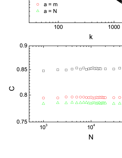
Figure 3: (Color online) Average clustering coefficient $C$ as a function of $k$ (a) and $N$ (b), respectively. The parameter $m=50$ for all plots.

The “complexity”of networks usually cannot be fully characterized by the degree distribution of vertices. Instead, the self-organization of structures of complex networks is mathematically encoded in various correlations existing among different vertices. To describe the network structure in more detail, several other topological quantities have been introduced to the statistics of networks, such as clustering coefficient, degree correlation, shortest path length, and so on. In the following, we shall go beyond the degree distribution and discuss those quantities.

Let us start with the clustering coefficient $C$ of the network, which is defined as the average probability with which two neighbors of a vertex are also neighbors to each other. For example, if a vertex $i$ has $k_{i}$ edges, and among its $k_{i}$ nearest neighbors there are $e_{i}$ edges, then the clustering coefficient of $i$ is defined by

$$C_{i}=\frac{2e_{i}}{k_{i}(k_{i}-1)}.$$ (9)

In order to compute the clustering coefficient, we shall consider the network as undirected and denote by $k=k^{\text{in}}+m$ the total degree of vertex $i$. In the deactivation model, new edges are created between the active vertices and the added one. Moreover, all the active vertices are connected. At each time step, the degree $k_{i}$ of each active vertex $i$ increases by $1$ and $e_{i}$ increase by $m-1$. Therefore, the evolutionary dynamics of $k_{i}$ and $e_{i}$ are given by

$$k_{i} = m+t,$$ (10)

$$\frac{de_{i}}{dt} = m-1.$$ (11)

Integrating Eq. (11) with the boundary condition $e_{i}(0)=m(m-1)/2$ and substituting the solution into Eq. (9), we recover the clustering coefficient $C(k)$ restricted to the vertices of degree $k$ KE02b ; VBMPV03 ,

$$C(k)=\frac{2(m-1)}{k-1}-\frac{m(m-1)}{k(k-1)}.$$ (12)

The expression indicates that the local clustering scales as $C(k)\sim k^{-1}$ for large $k$. In Fig. 3(a) we plot the average clustering coefficient $C(k)$ as a function of the vertex degree $k$. The best linear fit gives $C(k)\sim k^{-\xi}$ with exponent $\xi=0.98(6)$, which coincides with the prediction of Eq. (12). This is the signature of a nontrivial architecture in which low-degree vertices generically belong to well interconnected communities while high-degree ones are linked to many sites that may belong to different groups which are sparsely connected. In Fig. 3(b) we present three typical curves of the average clustering coefficient $C$ versus the network size $N$. It is worth noting that the clustering coefficient of the generated networks for all cases is higher than that for the corresponding one-dimensional regular lattices whose value is $3/4$ in the limit case Note2 .

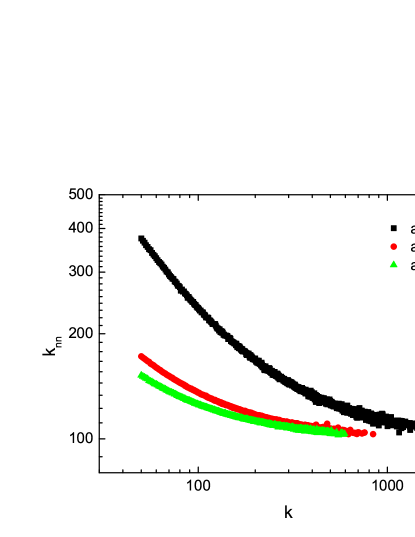
Figure 4: (Color online) Average nearest-neighbor degree $k_{nn}$ as a function of the vertex degree $k$ for different values of the bias $a$. The network parameters are $N=10^{5}$ and $m=50$.

Another commonly studied topological quantity is the degree correlation (or the mixing pattern), which can be characterized by analyzing the average degree of nearest neighbors, defined by PVV01

$$k_{nn,i}=\frac{1}{k_{i}}\sum_{j}a_{ij}k_{j}.$$ (13)

If $k_{nn,i}$ does not show any dependence on the degree of $i$, the network is uncorrelated. In case $k_{nn,i}$ is dependent on the vertex degree $i$, there are two kinds of correlations. If $k_{nn,i}$ increases with $k$, the network is assortative mixing; i.e., vertices with high connectivity will connect preferably to highly connected ones. If $k_{nn,i}$ decreases with $k$, the network is disassortative mixing; i.e., vertices with high connectivity will connect preferably to lowly connected ones MN02 . In Fig. 4 we show the simulation results of the average degree of nearest neighbors $k_{nn}$ as a function of $k$ for different values of $a$. In all cases, the degree correlation in the deactivation model is disassortative.

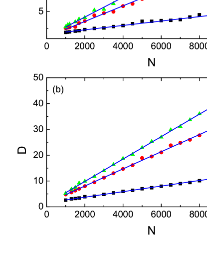
Figure 5: (Color online) Scaling of the average shortest path length (a) and the diameter (b) for different values of the bias $a$: $a=0$ (squares), $m$ (closed circles), and $N$ (triangles), respectively. The parameter $m=50$ for all plots.

To complete our study of the model, we finally investigate the scaling of the shortest path length and the diameter of the network. The shortest path length between two vertices is defined as the minimum number of intermediate vertices that must be traversed to go from vertex to vertex. The average shortest path length is the shortest path length averaged over all the possible pairs of vertices in the network. On the contrary, the diameter is defined as the largest among the shortest paths between any two vertices in the network VBMPV03 . In Fig. 5 we show the scaling behavior of the average shortest path length $L$ and the diameter $D$ of the resulting network. Both quantities grow linearly with the network size $N$ similar to one-dimensional regular lattices. That is to say, the deactivation model does not exhibit small-world properties. It indicates that there are very few effective shortcuts to reduce the distance although the network is highly clustered. However, the chainlike structure of the model does not necessarily mean large values of $L$ and $D$. Here $L$ and $D$ are still relatively small compared with $N$, especially for the case $a=0$.

In summary, we have suggested a rank-dependent deactivation mechanism and studied its influence on network growth. The resulting network shows several good features. (i) The degree distribution $N(k)$ of vertices is power law, which indicates the heterogeneous topology. (ii) The clustering coefficient is larger than that of one-dimensional regular lattices. Besides, the local clustering scales as $C(k)\sim k^{-1}$ for large $k$. (iii) The decay of the average degree of nearest neighbors $k_{nn}$ with $k$ characterizes the disassortative mixing pattern. (iv) The average shortest path length and the diameter grow with the network size, which results from deactivating sites during network evolution. Most of above properties have been found very common in realistic systems. We hope that the measurement conducted in present work could be applied to real networks in the empirical study. The model we have explored, however, is possibly the simplest one in the class of rank-dependent deactivation growing networks. One can notice that in our model the out-degree of the vertices remain unchanged during the whole evolving period, which is likely unreasonable for citation networks. Furthermore, many networks are intrinsically weighted, their edges having different strengths BBPV04 . Naturally one can generalize the present model to the weighted case and sort ranks by the vertex strength or fitness. There exists a series of improvements to be made in the future.

The authors acknowledge financial support from NSFC (Grant No. 10805033) and STCSM (Grant No. 08ZR1408000). This work was sponsored by the Innovation Foundation of Shanghai University.

References

- (1) D. J. Watts and S. H. Strogatz, Nature (London) 393, 440 (1998).
- (2) R. Albert and A.-L. Barabási, Rev. Mod. Phys. 74, 47 (2002).
- (3) L. D. F. Costa, F. A. Rodrigues, G. Travieso, and P. R. V. Boas, Adv. Phys. 56, 167 (2007).
- (4) S. Boccaletti, V. Latora, Y. Moreno, M. Chavez, and D.-U. Hwang, Phys. Rep. 424, 175 (2006).
- (5) S. N. Dorogovtsev, A. V. Goltsev, and J. F. F. Mendes, Rev. Mod. Phys. 80, 1275 (2008).
- (6) L. A. N. Amaral, A. Scala, M. Barthélemy, and H. E. Stanley, Proc. Natl. Acad. Sci. U.S.A. 97, 11149 (2000).
- (7) A.-L. Barabási and R. Albert, Science 286, 509 (1999).
- (8) S. N. Dorogovtsev and J. F. F. Mendes, Phys. Rev. E 62, 1842 (2000).
- (9) H. Zhu, X.-R. Wang, and J.-Y. Zhu, Phys. Rev. E 68, 056121 (2003).
- (10) K. B. Hajra and P. Sen, Phys. Rev. E 70, 056103 (2004).
- (11) A. Herdaǧdelen, E. Aygün, and H. Bingol, EPL 78, 60007 (2007).
- (12) R. Lambiotte, J. Stat. Mech. (2007), P02020.
- (13) S. N. Dorogovtsev, P. L. Krapivsky, and J. F. F. Mendes, Europhys. Lett. 81, 30004 (2008).
- (14) N. Crokidakis and M. A. de Menezes, J. Stat. Mech. (2009), P04018.
- (15) K. Klemm and V. M. Eguíluz, Phys. Rev. E 65, 036123 (2002).
- (16) K. Klemm and V. M. Eguíluz, Phys. Rev. E 65, 057102 (2002).
- (17) S. Fortunato, A. Flammini, and F. Menczer, Phys. Rev. Lett. 96, 218701 (2006).
- (18) L. Tian and D.-N. Shi, Eur. Phys. J. B 56, 167 (2007).
- (19) According to the model definition, vertices of large rank have high possibility to gain new edges, resulting in high degree.
- (20) R. J. Williams and N. D. Martinez, Nature (London) 404, 180 (2000).
- (21) M. E. J. Newman, Proc. Natl. Acad. Sci. USA 98, 404 (2001).
- (22) A. Vázquez, M. Boguñá, Y. Moreno, R. Pastor-Satorras, and A. Vespignani, Phys. Rev. E 67, 046111 (2003).
- (23) The clustering coefficient of the one-dimensional regular lattice with the coordination number is , which closes to 3/4 as increases.
- (24) R. Pastor-Satorras, A. Vázquez, and A. Vespignani, Phys. Rev. Lett. 87, 258701 (2001).
- (25) M. E. J. Newman, Phys. Rev. Lett. 89, 208701 (2002).
- (26) A. Barrat, M. Barthélemy, R. Pastor-Satorras, and A. Vespignai, Proc. Natl. Acad. Sci. U.S.A. 101, 3747 (2004).