Emission line taxonomy and the nature of AGN-looking galaxies in the SDSS

Abstract

Massive spectroscopic surveys like the SDSS have revolutionized the way we study AGN and their relations to the galaxies they live in. A first step in any such study is to define samples of different types of AGN on the basis of emission line ratios. This deceivingly simple step involves decisions on which classification scheme to use and data quality censorship. Galaxies with weak emission lines are often left aside or dealt with separately because one cannot fully classify them onto the standard Star-Forming, Seyfert of LINER categories. This contribution summarizes alternative classification schemes which include this very numerous population. We then study how star-formation histories and physical properties of the hosts vary from class to class, and present compelling evidence that the emission lines in the majority of LINER-like systems in the SDSS are not powered by black-hole accretion. The data are fully consistent with them being galaxies whose old stars provide all the ionizing power needed to explain their line ratios and luminosities. Such retired galaxies deserve a place in the emission line taxonomy.

1 Introduction

The way things are named plays an important role in the organization of scientific data. When a galaxy is described as “Star-Forming” (SF), one is lead to believe that star-formation is the dominant (or maybe the only) source of energy. When someone says a galaxy is a “LINER”, you are driven to think of a low luminosity AGN, powered by accretion (possibly in a radiatively inefficient regime) onto a super-massive black hole. Likewise, the word “Seyfert” works like an adjective to which one associates a vigorous AGN, a dusty torus which blocks our view of the nucleus, a bright and highly ionized Narrow Line Region, etc. Depending on the reader’s age range, memories of all those talks and papers about NGC 1068 will come to mind. Similarly, “SF $+$ AGN composite” brings to mind beasts like Mrk 477 (Heckman et al. 1997) or NGC 5135 (González Delgado et al. 2001), where star formation and AGN with comparable powers coexist.

In the context of in-depth studies of individual sources (like those presented in the contributions by Steiner and Storchi-Bergmann in this volume), such denominations are irrelevant formalities which play little (if any) role in the interpretation of the data. On the contrary, in the context of statistical studies of massive samples, where one trades quality and detail by quantity, taxonomy plays a key part. This paper, as many others in this volume and in the current literature, deals with this kind of data. The link with the central theme of this meeting, the co-evolution of central black holes and galaxies, is that in order use survey-quality data to study such a complex issue one must first make sure that black hole activity can be correctly identified and quantified.

The way one identifies AGN in massive optical spectroscopic samples like the SDSS is through their emission lines. Newcomers may have the impression that all that could be said and done about spectral classification of galaxies with emission lines has already been said and done. We first remind the reader that an awful lot of emission line galaxies (ELGs) in the SDSS simply cannot be reliably classified using standard classification schemes because some of the required lines (specially H$\beta$, but also [O iii]) are just too weak (§2). After reviewing current classification schemes (§3), we then present alternative diagnostic diagrams (and corresponding equations for class division boundaries) which allow placing this large population of Weak Line Galaxies (WLGs) within SF, Seyfert and LINER classes (§4). Cid Fernandes et al. (2010, CF10) opens up details on this revised taxonomy. Finally (§5 & §6), we take advantage of our detailed stellar population and emission line analysis of the whole SDSS DR7 (soon available at www.starlight.ufsc.br) to make the bridge between emission line classification and physical properties of the host. This leads to a surprising interpretation as to the nature of SDSS LINERs…

2 Weak Line Galaxies: Examples and the size of the problem

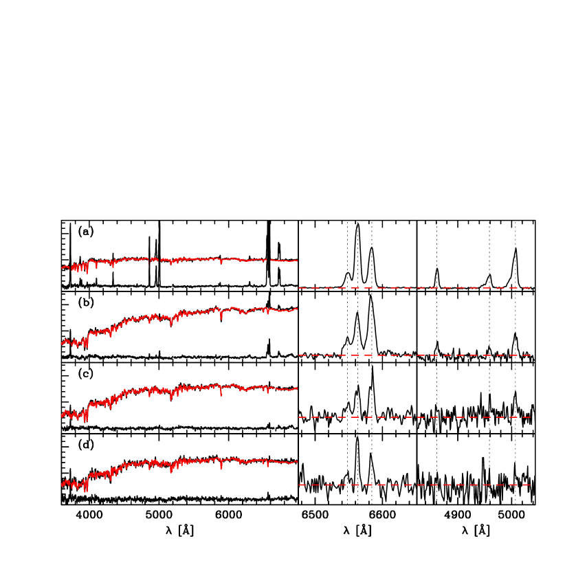
Figure 1: Example SDSS spectra, including our starlight fits and the residual spectra. The right panels are zooms of the pure emission spectra around H$\alpha$ and H$\beta$ (the dashed horizontal line marks the zero flux level). The top two are easily classifiable, but the bottom ones are not.

Fig. 1 shows four SDSS spectra. The top one is the spectral classifier’s dream. Its emission lines are so strong that one could tell it is a Seyfert 2 from miles away. Example b has weaker lines, but still strong enough for an unambiguous classification. From its H$\beta$, [O iii], H$\alpha$ and [N ii] fluxes, all of which are detected at 3 sigma or better confidence, one can confidently put this galaxy in the LINER’s bin. Things get tougher in example c, where [O iii], H$\alpha$ and [N ii] are all detected at $S/N\geq 3$, but H$\beta$ is not. Example d is even worse, as neither H$\beta$ nor [O iii] have decent detections.

Close to 80% of galaxies in the SDSS have H$\alpha$ and [N ii] lines detected at $S/N\geq 3$, but $\sim 1/3$ of these have less convincing detections of either or both of H$\beta$ and [O iii]. Cases c and d in Fig. 1 illustrate these WLGs. They are the spectral classifier’s nightmare. From the high [N ii]/H$\alpha$ one can be reasonably certain that these are AGN-like systems, but there is no well established method to diagnose whether these are Seyferts or LINERs. As many as 2/3 of the sources with $\log[\rm{N}\,\textsc{ii}]/{\rm H}\alpha>-0.2$ have weak H$\beta$ and/or [O iii].

Is there a way of rescuing this huge population from the classification limbo? The answer is yes. To do that, we must go back to the taxonomy drawing board.

3 BPT-based emission line taxonomy

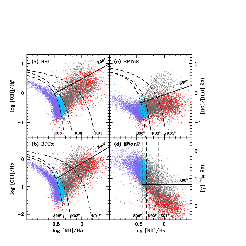
Figure 2: The BPT (top right) and three alternative diagnostic diagrams. Dashed lines show three widely used SF/AGN division lines (S06, K03 and K01), while the solid line divide Seyferts from LINERs (K06). A superscript “T” is used to denote dividing lines which were transposed from the originally defined (e.g., BPT-based) boundaries. See Table 1 for equations. Points in red have $S/N<3$ in either or both of H$\beta$ and [O iii] (WLGs).

According to the Oxford dictionary, taxonomy is the branch of science concerned with classification. The word finds its roots in the Greek, taxis meaning arrangement/order, and nomia meaning distribution. The ultimate icon of order in the distribution of emission lines properties of galaxies is the BPT diagram: $[\rm{O}\,\textsc{iii}]/{\rm H}\beta\times[\rm{N}\,\textsc{ii}]/{\rm H}\alpha$ (Fig. 2a). Its two well defined wings correspond to SF galaxies (left wing), and systems where the ionization source is harder than that produced by massive young stars (producing more energetic photo-electrons and thus enhanced collisionally excited lines). The right wing is commonly called the AGN wing, as this is where bona fide AGN are located.

Up until not so long ago a mixture of art (ad hoc curves) and science (grids of photoionization models) was used to draw class division lines in diagnostic diagrams like the BPT. The task of classifying ELGs on the basis of their emission line ratios was greatly simplified with the statistics of the SDSS. With so many points to plot, the morphology of diagnostic diagrams practically spells out class division boundaries, so that all one has to do is to find a suitable mathematical expression of this empirical result.

That is what Kauffmann et al. (2003, K03) did to separate SF galaxies from AGN in the BPT diagram. Their division line is the current standard SF/AGN classification scheme. Stasińska et al. (2006, S06) proposed a slightly different division line, based on photoionization models designed to match the upper boundary of the SF wing. Kewley et al. (2001, K01) proposed a model-based “extreme starburst” line which, as seen in Fig. 2a, does not match the observed morphology of the BPT at all. This line is nowadays widely used to isolate “pure AGN”, and, in combination with the K03 line, to define “SF $+$ AGN composite systems”, even though it was not designed to do either thing.

The separation of Seyferts from LINERS was revisited by Kewley et al. (2006, K06), who identified a split of sources in the right wing into upper (Seyfert) and lower (LINER) branches, clearly visible in diagrams like [O iii]/H$\beta$ $\times$ [O i]/H$\alpha$ or [S ii]/H$\alpha$ (also in the BPT, albeit more blurred). K06 devised a classification system based on H$\beta$, [O iii], [O i], H$\alpha$, [N ii] and [S ii] lines which tracks this observed bimodality. To convert their Seyfert/LINER classification scheme to a simpler one based exclusively on the BPT, a 2D version of the optimal separator method was employed, maximizing completeness and reliability fractions (see CF10). This leads to the solid line in Fig. 2a (see also Table 1).

We thus have 3 versions of SF/AGN division lines (S06, K03, K01, the latter of which is not really adequate to separate SF from AGN), plus the K06 Seyfert/LINER classification scheme transposed to a straight line in the BPT plane. Obviously, all of this only applies when one has reliable H$\beta$, [O iii], H$\alpha$ and [N ii] fluxes at hand. That is OK for examples a and b in Fig. 1, but not for c, d and the whole population of WLGs they represent. To include this forgotten population of ELGs one needs to devise classification schemes which are more economic in terms of data-quality (emission line $S/N$) requirements.

4 Emission line taxonomy revisited to include Weak Line Galaxies

Table 1: Class boundaries for spectral classification in various diagnostic diagrams

$x=\log\frac{[\rm{N}\,\textsc{ii}]}{{\rm H}\alpha}$		SF/AGN			Seyfert/LINER	%
Diagram	$y$	S06	K03	K01	K06	All1	AGN2
BPT	$\log\frac{[\rm{O}\,\textsc{iii}]}{{\rm H}\beta}$	$0.96+\frac{0.29}{x+0.20}$	$1.30+\frac{0.61}{x-0.05}$	$1.19+\frac{0.61}{x-0.47}$	$1.01x+0.48$	67	29
BPT$\alpha$	$\log\frac{[\rm{O}\,\textsc{iii}]}{{\rm H}\alpha}$	$0.46+\frac{0.29}{x+0.22}$	$0.68+\frac{0.49}{x+0.03}$	$0.69+\frac{0.57}{x-0.38}$	$1.20x-0.15$	81	57
BPTo2	$\log\frac{[\rm{O}\,\textsc{iii}]}{[\rm{O}\,\textsc{ii}]}$	$1.06+\frac{0.26}{x+0.24}$	$1.10+\frac{0.33}{x+0.11}$	$1.25+\frac{0.48}{x-0.21}$	$0.64x-0.06$	77	50
EW$\alpha$n2	$\log W_{{\rm H}\alpha}$	$x=-0.40$	$x=-0.32$	$x=-0.10$	$W_{{\rm H}\alpha}=6$ Å	100	100

Notes:
¹ Fraction of all galaxies which have $S/N\geq 3$ in all lines involved.
² Fraction of all AGN-like galaxies ($\log[\rm{N}\,\textsc{ii}]/{\rm H}\alpha>-0.2$) which have $S/N\geq 3$ in all lines involved.

The main challenge to classify WLGs is to find a replacement for H$\beta$, the weakest of the 4 BPT lines. H$\alpha$ and [O ii] provide suitable alternatives. They are much less affected by low $S/N$, and the [O iii]/H$\alpha$ and [O iii]/[O ii] ratios carry similar physical information content as [O iii]/H$\beta$ (with both caveats and advantages). This leads us to the BPT$\alpha$ and BPTo2 diagrams shown in Figs. 2b and c. The S06^T, K03^T, K01^T, and K06^T division lines in these more inclusive diagrams are optimal transpositions of the original S06, K03, K01 SF/AGN and the K06 Seyfert/LINER classification schemes. Equations for these lines are given in Table 1, which also shows that whereas in the BPT 67% of the ELGs can be classified on the basis of $S/N\geq 3$ data, in the BPTo2 and BTP$\alpha$ this fraction increases to 77 and 81%. The gain is much higher considering right wing galaxies alone, for which these diagrams allow one to classify about twice as many sources as the BPT.

A complete solution to the classification of WLGs requires replacing [O iii] by a stronger line with physically equivalent diagnostic power, but there is no such a thing. A different way of looking at emission lines is to combine line ratios and equivalent widths. It so happens that replacing [O iii]/H$\beta$ by the equivalent width of H$\alpha$ provides an efficient and very cheap classification scheme. In the EW$\alpha$n2 diagram (Fig. 2d), SF are separated from AGN by $[\rm{N}\,\textsc{ii}]/{\rm H}\alpha=-0.4$ for the S06 scheme and $-0.32$ for the K03 one, while Seyferts and LINERs split at $W_{{\rm H}\alpha}=6$ Å. Inevitably, the completeness and reliability fractions of these optimal transpositions are not as good as for other diagrams, meaning that the classifications obtained with this diagram do not match perfectly those obtained with more standard ones. Yet, given its much larger applicability, we dare suggesting the EW$\alpha$n2 diagram should replace the BPT as a basis for spectral classification. Those interested in AGN-host connections should welcome this proposition, as an equivalent width provides a more direct metric of such connections than a line flux ratio.

5 Star Formation Histories across the BPT and EW$\alpha$n2 diagrams

Figure 3: SFHs across the EW$\alpha$n2 diagram. Points and contours indicate the location of ELGs in the SDSS DR7. The diagrams is chopped into boxes containing $>500$ galaxies. The number at the top of each box is the median logarithm of the stellar mass (in M_⊙). The curves shows the $t$-by-$t$ median specific star-formation rate against the lookback time, as show in the inset. Thinner lines tracer the 16 and 84 percentiles. Dashed lines mark the transposed S06-SF/AGN and K06-Seyfert/LINER division lines. Based on studies of globular clusters, we warn that the small upturn in the SFHs of predominantly old systems at very young ages ($<10^{7}$ yr) may be a side effect of blue horizontal branches not included in the stellar population models.

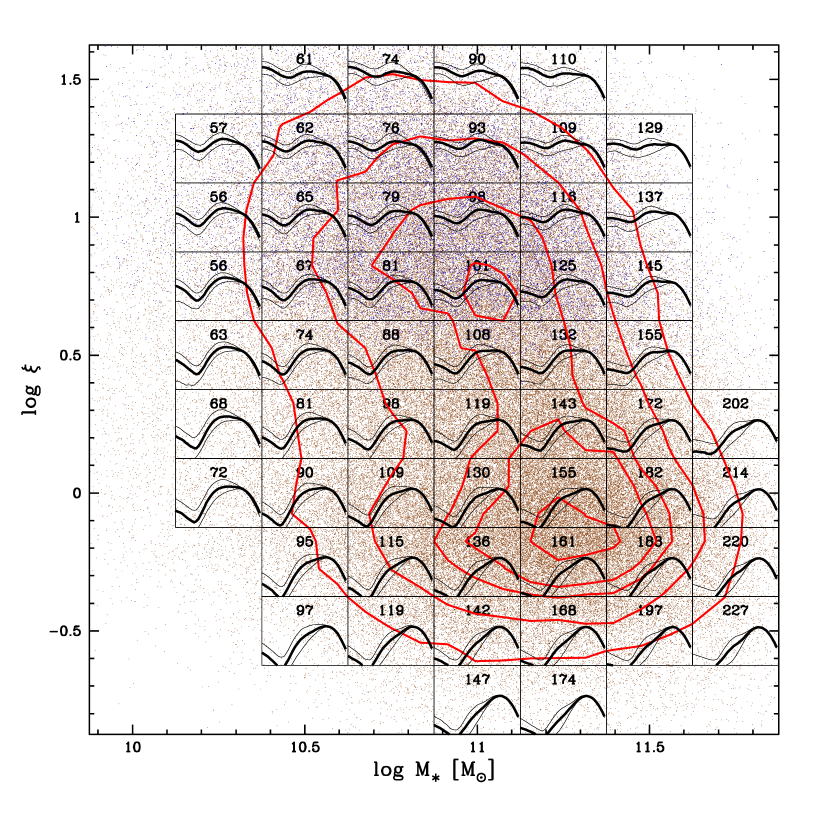
Figure 4: SFHs across the $M_{\star}$ versus $\xi$ diagram for galaxies classified as AGN according to the $\log[\rm{N}\,\textsc{ii}]/{\rm H}\alpha>-0.40$ criterion (S06^T in Fig. 2d). (The SFH curves are on the same scale as in Fig. 3.) Sources with $W_{{\rm H}\alpha}>6$ Å (Seyferts in the EW$\alpha$n2 diagram) are painted in blue. Numbers within each box represent the median $\sigma_{\star}$ (in km s^-1), believed to be a tracer of black-hole mass. Notice the bimodality in the $\xi$ distribution. $\xi\sim 1$ indicates galaxies whose H$\alpha$ luminosity can be entirely powered by its old stars, as in the retired galaxy model of S08. The SFH of galaxies in the $\xi\sim 1$ peak show that these systems have indeed stopped forming stars long ago.

So far we have talked only about emission line taxonomy. Yet, one should not loose sight of the fact that classifying galaxies is not a goal in itself, but just a means of organizing data in terms of observables which (hopefully) bear correspondence with the underlying physics, mapping different phenomena (or regimes of a same mechanism) onto different classes. As shown in previous papers by the SEAGal (Semi Empirical Analysis of Galaxies) collaboration, our starlight-SDSS database contains far more information than emission line properties. Stellar masses ($M_{\star}$), velocity dispersions ($\sigma_{\star}$), stellar extinction, mean ages, stellar metallicities and full time-dependent Star Formation Histories (SFHs) are among the most interesting ones. A gold-mine to examine the link between emission line classes and physical properties of host galaxies.

Stasińska’s contribution in this same volume shows the SFHs of strong line galaxies ($S/N\geq 3$ in all 4 BPT lines) across the BPT diagram. From top to bottom along the SF wing (and thus for increasing nebular metallicity) SFHs change from systems which are nowadays forming stars at a much higher pace than in the past to galaxies which have kept $\sim$ constant rates throughout their lives (Asari et al. 2007). Among AGN-looking galaxies, one sees that recent ($t<10^{8}$ yr) SF activity decreases strongly as one goes from Seyferts to LINERs.

That plot is heavily biased, particularly in the right wing, where $\sim 2$ in every 3 galaxies are left out because of bad H$\beta$ and/or [O iii] data (Table 1). To include these WLGs, let us see how SFHs look in our most inclusive diagnostic diagram: The EW$\alpha$n2. Overall, Fig. 3 confirms the general result obtained from the BPT, that Seyferts have substantial recent SF whereas LINERs do not. The main difference is that, as a result of removing the prejudice against WLGs, the population of LINERs is now much larger. With the exception of massive metal rich SF systems which have weak-[O iii], most WLGs are LINER-like systems, in the bottom-right part of the EW$\alpha$n2 diagram. LINERs with strong lines are just the tip of an iceberg.

6 Retired galaxies $=$ fake AGN

Plots like Fig. 3 can be made for any choice of axis. The abundant information provided by our stellar population analysis allows one to look at the data from less observable-oriented perspectives, so lets re-do that plot with more physically oriented variables. An obvious choice for a physically interesting x-axis is the stellar mass. Out of numerous options for the y-axis, for reasons which will soon become clear, we chose a rather unconventional one: The ratio of the observed H$\alpha$ luminosity to the predicted H$\alpha$ output due to photoionization by old stars ($t>10^{8}$ yr):

$$\xi=\frac{L_{{\rm H}\alpha}^{\rm observed}}{L_{{\rm H}\alpha}^{\rm predicted}(t>10^{8}\,{\rm yr})}$$

The denominator comes from our starlight analysis, which (with the aid of evolutionary synthesis models) allows us to predict the ionizing radiation field emanating from the old stars in a galaxy. Using case B recombination coefficients and neglecting escape of ionizing photons, one derives the predicted $L_{{\rm H}\alpha}$. Notice that this choice for an y-axis makes no statement about what powers the H$\alpha$ emission. The normalization of $L_{{\rm H}\alpha}^{\rm observed}$ by $L_{{\rm H}\alpha}^{\rm predicted}(t>10^{8}{\rm yr})$ can be seen as just a natural unit to measure the H$\alpha$ power.

Fig. 4 shows the $M_{\star}$ versus $\xi$ diagram. This being an AGN symposium, the plot is restricted to AGN-like systems, defined as those with $\log[\rm{N}\,\textsc{ii}]/{\rm H}\alpha>-0.40$. Of the many things that could be said about this plot, let us first highlight the bimodality in the “AGN” population, strongly reminiscent of the Seyfert/LINER dichotomy identified by K06 in their inspection of diagnostic diagrams. Indeed, Seyferts live at the top part of this diagram, while LINERs populate the $\xi<0.5$ region, peaking at $\xi$ slightly below 1.

$\xi=1$ means that exactly all H$\alpha$ photons can be explained as coming from photoionization by post-AGB stars and white dwarfs, ionizing sources which are seldom considered relevant, specially among AGNauts. It so happens that $\xi\sim 1$ is also the center of the low peak in the bimodal distribution of sources in Fig. 4. Looking at the SFHs of these galaxies one sees that they have retired from forming stars long ago. Given the factor of $10^{5}$ difference in ionizing fluxes for young ($t<10^{7}$ yr) and $>10^{8}$ yr populations, any ongoing SF, even at small levels, would move these galaxies to the $\xi\gg 1$ regime. Similarly (but on a more semantic vein), any AGN worth being called “active” should be able to produce an ionizing field stronger than that produced by the least powerful stellar populations. Hence, $\xi\sim 1$ galaxies really ought to be retired, and their central black holes must be fasting, otherwise $\xi$ would be higher.

But can retired galaxies mimic AGN? If you haven’t done so yet, this is the time to read Stasińska et al. (2008). The self-consistent stellar population $+$ photoionization models presented there show that retired galaxies can indeed mimic AGN in terms of emission line ratios and luminosities, and that about 1/4 of SDSS LINERs with $S/N\geq 3$ in all BPT lines can be explained in this way. Including WLGs, this fraction increases tremendously, to the point that the Seyfert/LINER dichotomy does not seem to be a manifestation of two regimes of black-hole accretion, but rather a consequence of two entirely different phenomena: non-stellar versus stellar ionization (ie, bona-fide AGN $\times$ retired galaxies, or true $\times$ fake AGN).

LINERs have long been known to comprise a rather mixed bag, some with unequivocal evidence of AGN (broad lines, variability, X-rays, etc.). Our claim is that the emission lines in most objects called LINERs in the SDSS are not powered by black-hole accretion, but by old stars. Hence, beware of fake AGN!

References

- [1]
- [Asari et al.(2007)] Asari, N. V., Cid Fernandes, R., Stasińska, G., Torres-Papaqui, J. P., Mateus, A., Sodré, L., Schoenell, W., & Gomes, J. M. 2007, MNRAS, 381, 263
- [Heckman et al.(1997)] Heckman, T. M., Gonzalez-Delgado, R., Leitherer, C., Meurer, G. R., Krolik, J., Wilson, A. S., Koratkar, A., & Kinney, A. 1997, ApJ, 482, 114
- [González Delgado et al.(2001)] González Delgado, R. M., Heckman, T., & Leitherer, C. 2001, ApJ, 546, 845
- [Kauffmann et al.(2003)] Kauffmann, G., et al. 2003, MNRAS, 346, 1055
- [Kewley et al.(2001)] Kewley, L. J., Dopita, M. A., Sutherland, R. S., Heisler, C. A., & Trevena, J. 2001, ApJ, 556, 121
- [Kewley et al.(2006)] Kewley, L. J., Groves, B., Kauffmann, G., & Heckman, T. 2006, MNRAS, 372, 961
- [Stasińska et al.(2006)] Stasińska, G., Cid Fernandes, R., Mateus, A., Sodré, L., & Asari, N. V. 2006, MNRAS, 371, 972
- [Stasińska et al.(2008)] Stasińska, G., Vale Asari, N., Cid Fernandes, R., Gomes, J. M., Schlickmann, M., Mateus, A., Schoenell, W., & Sodré, L., Jr. 2008, MNRAS, 391, L29