Magnetofluid dynamics of magnetized cosmic plasma: firehose and gyrothermal instabilities

Abstract

Both global dynamics and turbulence in magnetized weakly collisional cosmic plasmas are described by general magnetofluid equations that contain pressure anisotropies and heat fluxes that must be calculated from microscopic plasma kinetic theory. It is shown that even without a detailed calculation of the pressure anisotropy or the heat fluxes, one finds the macroscale dynamics to be generically unstable to microscale Alfvénically polarized fluctuations. Two instabilities that can be treated this way are considered in detail: the parallel firehose instability (including the finite-Larmor-radius effects that determine the growth rate and scale of the fastest growing mode) and the gyrothermal instability (GTI). The latter is a new result — it is shown that a parallel ion heat flux destabilizes Alfvénically polarized fluctuations even in the absence of the negative pressure anisotropy required for the firehose. The main physical conclusion is that both pressure anisotropies and heat fluxes associated with the macroscale dynamics trigger plasma microinstabilities and, therefore, their values will likely be set by the nonlinear evolution of these instabilities. Ideas for understanding this nonlinear evolution are discussed. It is argued that cosmic plasmas will generically be “three-scale systems,” comprising global dynamics, mesoscale turbulence and microscale plasma fluctuations. The astrophysical example of cool cores of galaxy clusters is considered quantitatively and it is noted that observations point to turbulence in clusters (velocity, magnetic and temperature fluctuations) being in a marginal state with respect to plasma microinstabilities and so it is the plasma microphysics that is likely to set the heating and conduction properties of the intracluster medium. In particular, a lower bound on the scale of temperature fluctuations implied by the GTI is derived.

1 Introduction

Many astrophysical plasmas are not sufficiently collisional to be described by the standard fluid equations of magnetohydrodynamics (MHD) (see, e.g., Balbus, 2004; Schekochihin & Cowley, 2006; Sharma et al., 2006, 2007). When the collision frequency $\nu$ is smaller than the Larmor frequency $\Omega=eB/mc$ of the particle gyration about the magnetic-field lines, the plasma becomes magnetized: pressure and heat flux are now tensors that depend on the local direction of the magnetic field. This complication leads to three significant physical effects. Firstly, on the macroscopic scales, the momentum and heat transport become highly anisotropic with respect to the magnetic-field direction. Secondly, old MHD instabilities, like the MRI, that are believed to excite turbulence in astrophysical systems (Balbus & Hawley, 1998), are significantly modified (Quataert et al., 2002; Sharma et al., 2003; Islam & Balbus, 2005) and new ones appear: MTI (Balbus, 2000), MVI (Balbus, 2004), HBI (Quataert, 2008). Thirdly, a host of superfast microscale instabilities exist that are directly driven by the pressure anisotropies (see Schekochihin et al., 2005; Sharma et al., 2006, and references therein) and, as we are about to discover, also by heat fluxes.

The presence of microscale instabilities especially opens a fundamental problem: the equations one tends to use to describe the macroscopic dynamics of magnetized plasma, be they fluid or kinetic, are derived in the long-wavelength limit ($k\rho\ll 1$, where $\rho$ is the Larmor radius; see Kulsrud, 1983) and turn out to be ill-posed because in this limit the microinstabilities have growth rates proportional to $k$ (Schekochihin et al., 2005). In order to regularize them at small scales, one has to take into account effects associated with the finite Larmor radius (FLR), which requires fairly complicated kinetic theory and typically means that the full multiscale problem is analytically hard and numerically intractable. Ideally, one would like to have an effective mean-field theory, with the microscale fluctuations analytically averaged to produce some form of closure for the momentum and heat transport. This has not been achieved yet, but an educated guess about the form of such a closure can me made, based on the idea that the system should always find itself in the marginal state with respect to the microinstabilities (Sharma et al., 2006, 2007; Schekochihin & Cowley, 2006; Lyutikov, 2007; Kunz et al., 2010).

In this paper, we attempt to make progress in setting up the theoretical framework for astrophysical plasma dynamics by addressing three basic questions: what is the general form of the dynamical equations that we are attempting to approximate? what can be learned about the microinstabilities under the most general assumptions? what constraints do their marginal stability conditions impose on the allowed macroscopic states of the plasma? The first of these questions is addressed in section 2, the second in section 3, where an old (firehose) and a new (gyrothermal) instabilities of Alfvénically polarized perturbations are derived. Possible ways of thinking about the nonlinear physics of these microinstabilities are proposed in section 4. The physical conclusions are summarized in section 5, including a discussion of the relevance of all this in galaxy cluster cores (as a case study of a multiscale astrophysical plasma system).

2 Equations for plasma dynamics

Let us consider a two-species fully ionized plasma. In the completely general case (assuming only quasineutrality), the evolution of ion density $n$ and flow velocity $\mn@boldsymbol{u}$ is governed by the following equations

$$\frac{\mathrm{d}n}{\mathrm{d}t}=-n\mn@boldsymbol{\nabla}\cdot\mn@boldsymbol{u},$$ (1)

$$mn\,\frac{\mathrm{d}\mn@boldsymbol{u}}{\mathrm{d}t}=-\mn@boldsymbol{\nabla}\cdot\left(\textbf{{P}}+\textbf{{I}}\,\frac{B^{2}}{8\pi}-\frac{\mn@boldsymbol{B}\mn@boldsymbol{B}}{4\pi}\right),$$ (2)

where $m$ is the ion mass, $\mathrm{d}/\mathrm{d}t=\partial/\partial t+\mn@boldsymbol{u}\cdot\mn@boldsymbol{\nabla}$ the convective derivative, I the unit dyadic, $\mn@boldsymbol{B}$ the magnetic field and P the plasma pressure tensor. It is via P that all the kinetic physics comes in: in general, P is the sum of the ion and electron pressures and for each species, it is $\textbf{{P}}=m\int d^{3}\mn@boldsymbol{v}\,\mn@boldsymbol{v}\mn@boldsymbol{v}f$, calculated from the distribution function $f(t,\mn@boldsymbol{r},\mn@boldsymbol{v})$, which is the solution of the kinetic equation for that species. Note that $\mn@boldsymbol{v}$ is the peculiar velocity, i.e., the particle’s velocity in a frame moving with the mean flow velocity $\mn@boldsymbol{u}$.

Thus, the challenge is to calculate P. This typically involves setting up an asymptotic expansion of the kinetic equation with respect to one or several of the small parameters available for the plasma under the set of macroscopic conditions of interest. Many such expansions for magnetized plasma exist, corresponding to various physical regimes: collisional (Braginskii, 1965; Mikhailovskii & Tsypin, 1971, 1984; Catto & Simakov, 2004), long-wavelength collisionless, or drift-kinetic (Chew et al., 1956; Kulsrud, 1983), short-wavelength anisotropic, or gyrokinetic (Howes et al., 2006; Schekochihin et al., 2009, and references therein), and more specialized versions of the above, appropriate for the treatment of pressure-anisotropy-driven instabilities: firehose (Schekochihin et al., 2008; Rosin et al., 2010) and mirror (Califano et al., 2008; Istomin et al., 2009; Rincon et al., 2010). We do not at the moment wish to pick any one of these, but simply notice that in all of them, the equilibrium distribution function invariably turns out to be gyrotropic, i.e., independent of the phase angle of the particle’s Larmor gyration. The only assumptions needed for that is that the characteristic frequencies $\omega$ for the evolution both of the equilibrium and of the perturbations thereof should be smaller than the ion Larmor frequency $\Omega$ and the length scales of the equilibrium longer than the ion Larmor radius $\rho$. If the pressure tensor is assumed to be determined purely by the gyrotropic lowest-order distribution, then it reduces to a diagonal form, $\textbf{{P}}=p_{\perp}(\textbf{{I}}-\mn@boldsymbol{b}\mn@boldsymbol{b})+p_{\parallel}\mn@boldsymbol{b}\mn@boldsymbol{b}$, where $\mn@boldsymbol{b}=\mn@boldsymbol{B}/B$, and the perpendicular and parallel pressures are $p_{\perp}=m\int\mathrm{d}^{3}\mn@boldsymbol{v}\,(v_{\perp}^{2}/2)f$ and $p_{\parallel}=m\int\mathrm{d}^{3}\mn@boldsymbol{v}\,v_{\parallel}^{2}f$. These pressures can be shown to satisfy the so-called CGL equations: for each particle species, they are (Chew et al. 1956; Kulsrud 1983; Snyder et al. 1997; see Appendix B for a simple derivation)

$$p_{\perp}\frac{\mathrm{d}}{\mathrm{d}t}\ln\frac{p_{\perp}}{nB}=-\mn@boldsymbol{\nabla}\cdot\mn@boldsymbol{q}_{\perp}-q_{\perp}\mn@boldsymbol{\nabla}\cdot\mn@boldsymbol{b}-\nu(p_{\perp}-p_{\parallel}),$$ (3)

$$p_{\parallel}\frac{\mathrm{d}}{\mathrm{d}t}\ln\frac{p_{\parallel}B^{2}}{n^{3}}=-\mn@boldsymbol{\nabla}\cdot\mn@boldsymbol{q}_{\parallel}+2q_{\perp}\mn@boldsymbol{\nabla}\cdot\mn@boldsymbol{b}-2\nu(p_{\parallel}-p_{\perp}),$$ (4)

where $\nu$ is the collision frequency, $q_{\perp}=m\int\mathrm{d}^{3}\mn@boldsymbol{v}\,v_{\parallel}(v_{\perp}^{2}/2)f$ and $q_{\parallel}=m\int\mathrm{d}^{3}\mn@boldsymbol{v}\,v_{\parallel}^{3}f$ are the parallel fluxes of the perpendicular and parallel heat and $\mn@boldsymbol{q}_{\perp}=\mn@boldsymbol{b}q_{\perp}$, $\mn@boldsymbol{q}_{\parallel}=\mn@boldsymbol{b}q_{\parallel}$.

As mentioned above, pressure anisotropies $p_{\perp}-p_{\parallel}\neq 0$ lead to instabilities whose peak growth rates occur at scales smaller than those allowed by the validity of the diagonal approximation for P and are not captured by this approximation (Schekochihin et al., 2005). The instabilities are regularized by the FLR effects, so it is natural to resort to FLR corrections in the plasma pressure tensor (Snyder & Hammett, 2001; Ramos, 2005; Passot & Sulem, 2007). To lowest order in $\omega/\Omega$ and $k\rho_{i}$, this is quite easy to do and the result, a simple derivation of which is given in Appendix A, is

P $$= p_{\perp}\textbf{{I}}-(p_{\perp}-p_{\parallel})\mn@boldsymbol{b}\mn@boldsymbol{b}+\textbf{{G}},$$ (5)

G $$= \frac{1}{4\Omega}\bigl{[}\mn@boldsymbol{b}\times\textbf{{S}}\cdot\left(\textbf{{I}}+3\mn@boldsymbol{b}\mn@boldsymbol{b}\right)-\left(\textbf{{I}}+3\mn@boldsymbol{b}\mn@boldsymbol{b}\right)\cdot\textbf{{S}}\times\mn@boldsymbol{b}\bigr{]}$$ (6)

$$+\,\frac{1}{\Omega}\bigl{[}\mn@boldsymbol{b}\left(\mn@boldsymbol{\sigma}\times\mn@boldsymbol{b}\right)+\left(\mn@boldsymbol{\sigma}\times\mn@boldsymbol{b}\right)\mn@boldsymbol{b}\bigr{]},$$

where the auxiliary tensor S and vector $\mn@boldsymbol{\sigma}$ are

S $$= \left(p_{\perp}\mn@boldsymbol{\nabla}\mn@boldsymbol{u}+\mn@boldsymbol{\nabla}\mn@boldsymbol{q}_{\perp}\right)+\left(p_{\perp}\mn@boldsymbol{\nabla}\mn@boldsymbol{u}+\mn@boldsymbol{\nabla}\mn@boldsymbol{q}_{\perp}\right)^{T},$$ (7)

$$\mn@boldsymbol{\sigma} = (p_{\perp}-p_{\parallel})\left(\frac{\mathrm{d}\mn@boldsymbol{b}}{\mathrm{d}t}+\mn@boldsymbol{b}\cdot\mn@boldsymbol{\nabla}\mn@boldsymbol{u}\right)+(3q_{\perp}-q_{\parallel})\mn@boldsymbol{b}\cdot\mn@boldsymbol{\nabla}\mn@boldsymbol{b}.$$ (8)

Each plasma species contributes a pressure tensor of the form (5). In general, electron pressures are comparable to ion pressures, but it is not hard to show that the electrons’ contribution to the FLR term G is smaller than the ions’ by a factor of $(m_{e}/m_{i})^{1/2}$.

Note that if one sets $p_{\perp}-p_{\parallel}=0$ and $3q_{\perp}-q_{\parallel}=0$ (as would be the case for an isotropic equilibrium distribution and collisional heat fluxes), the FLR term G in equation (5) is readily recognized as the so called “gyroviscosity” tensor, first obtained (in the collisional limit) by Braginskii (1965) (he assumed sonic flows and found just the $\mn@boldsymbol{\nabla}\mn@boldsymbol{u}$ terms; the heat flux terms were introduced later by Mikhailovskii & Tsypin (1971, 1984) to accommodate subsonic flows).

Thus, the momentum equation (LABEL:eq:mom) has the form

$$mn\,\frac{\mathrm{d}\mn@boldsymbol{u}}{\mathrm{d}t} = -\mn@boldsymbol{\nabla}\left(p_{\perp}+\frac{B^{2}}{8\pi}\right)$$ (9)

$$+\,\mn@boldsymbol{\nabla}\cdot\left[\mn@boldsymbol{b}\mn@boldsymbol{b}\left(p_{\perp}-p_{\parallel}+\frac{B^{2}}{4\pi}\right)-\textbf{{G}}\right],$$

where G is given by equation (6). Now we need an evolution equation for the magnetic field. Faraday’s law reads

$$\frac{\partial\mn@boldsymbol{B}}{\partial t}=-c\mn@boldsymbol{\nabla}\times\mn@boldsymbol{E},$$ (10)

where $\mn@boldsymbol{E}$ is the electric field. The electron momentum equation is used to calculated $\mn@boldsymbol{E}$. Since the electron mass is small compared to the ion mass, to lowest order in $(m_{e}/m_{i})^{1/2}$ this reduces to the force balance

$$-\mn@boldsymbol{\nabla}\cdot\textbf{{P}}_{e}-en_{e}\left(\mn@boldsymbol{E}+\frac{\mn@boldsymbol{u}_{e}\times\mn@boldsymbol{B}}{c}\right)=0.$$ (11)

The electron density $n_{e}$ is related to the ion density $n$ by the quasineutrality of the plasma, $n_{e}=Zn$ (the ion charge is $Z$ times electron charge $e$). The electron flow velocity $\mn@boldsymbol{u}_{e}$ is related to the ion flow velocity $\mn@boldsymbol{u}$ by $\mn@boldsymbol{u}_{e}=\mn@boldsymbol{u}-\mn@boldsymbol{j}/en_{e}$, where, using Ampère’s law, the current density is $\mn@boldsymbol{j}=c\mn@boldsymbol{\nabla}\times\mn@boldsymbol{B}/4\pi$. Finally, since the FLR terms in the electron pressure tensor are negligible to lowest order in $(m_{e}/m_{i})^{1/2}$, we have $\textbf{{P}}_{e}=p_{\perp e}\textbf{{I}}-(p_{\perp e}-p_{\parallel e})\mn@boldsymbol{b}\mn@boldsymbol{b}$. Assembling all this together, we get

$$\frac{\mathrm{d}\mn@boldsymbol{B}}{\mathrm{d}t} = \mn@boldsymbol{B}\cdot\mn@boldsymbol{\nabla}\mn@boldsymbol{u}-\mn@boldsymbol{B}\mn@boldsymbol{\nabla}\cdot\mn@boldsymbol{u}-c\mn@boldsymbol{\nabla}\times\mn@boldsymbol{\tilde{E}},$$ (12)

$$\mn@boldsymbol{\tilde{E}} = -\frac{1}{en_{e}}\mn@boldsymbol{\nabla}\left(p_{\perp e}+\frac{B^{2}}{8\pi}\right)$$ (13)

$$+\frac{1}{en_{e}}\mn@boldsymbol{\nabla}\cdot\left[\mn@boldsymbol{b}\mn@boldsymbol{b}\left(p_{\perp e}-p_{\parallel e}+\frac{B^{2}}{4\pi}\right)\right].$$

Note that $c/en_{e}=B/mn\Omega$, where $m$, $n$ and $\Omega$ are ion mass, density and Larmor frequency, respectively.

We will not be preoccupied here with the determination of the pressures and heat fluxes (which is necessary to close the set of equations we have written down). Depending on the physical regime one is interested in, they can either be calculated in the collisional limit (Braginskii, 1965) or Landau fluid closures can be devised for them, appropriate for a collisionless plasma (Snyder et al., 1997; Snyder & Hammett, 2001; Ramos, 2005; Passot & Sulem, 2007). Instead of wading into this rather complex subject, we will inquire what can be learned just from the general form of the equations of plasma dynamics outlined above.

3 Firehose and gyrothermal instabilities

In any given astrophysical problem, one might find some macroscale solution of the equations of section 2, describing the large-scale dynamics. Such solutions turn out to be generically unstable to perturbations with large wavenumbers and high frequencies (much larger than the fluid turnover rates $\omega\gg|\mn@boldsymbol{\nabla}\mn@boldsymbol{u}|$). In general, showing this involves having to perturb all quantities, including the pressures and the heat fluxes, which requires a kinetic closure. However, there is a class of perturbations whose stability does not depend on the details of kinetic theory.

Let us start by perturbing the momentum equation (9). We assume the perturbation to be $\propto\exp(-i\omega t+i\mn@boldsymbol{k}\cdot\mn@boldsymbol{r})$. In our perturbation theory, we will always consider terms containing $\omega$ and $\mn@boldsymbol{k}$ to be dominant in comparison with the terms containing time derivatives or gradients of the macroscale quantities. Thus, from equation (9), we get, noting that $\mn@boldsymbol{\nabla}\cdot\mn@boldsymbol{B}=0$ implies $\mn@boldsymbol{\nabla}\cdot\mn@boldsymbol{b}=-\mn@boldsymbol{b}\cdot\mn@boldsymbol{\nabla}B/B$,

$$mn\omega\delta\mn@boldsymbol{u} = \mn@boldsymbol{k}_{\perp}\left(\delta p_{\perp}+\frac{B\delta B}{4\pi}\right)+\mn@boldsymbol{b}k_{\parallel}\left[(p_{\perp}-p_{\parallel})\frac{\delta B}{B}+\delta p_{\parallel}\right]$$ (14)

$$-\,k_{\parallel}\left(p_{\perp}-p_{\parallel}+\frac{B^{2}}{4\pi}\right)\delta\mn@boldsymbol{b}+\mn@boldsymbol{k}\cdot\delta\textbf{{G}}.$$

Note that $\delta\textbf{{S}}=ip_{\perp}(\mn@boldsymbol{k}\delta\mn@boldsymbol{V}+\delta\mn@boldsymbol{V}\mn@boldsymbol{k})$, where $\delta\mn@boldsymbol{V}=\delta\mn@boldsymbol{u}+(q_{\perp}\delta\mn@boldsymbol{b}+\mn@boldsymbol{b}\delta q_{\perp})/p_{\perp}$. Therefore, from equation (6),

$$\mn@boldsymbol{k}\cdot\delta\textbf{{G}}=\frac{ip_{\perp}}{\Omega}\bigg{\{}\left(k_{\parallel}^{2}+\frac{k_{\perp}^{2}}{4}\right)(\mn@boldsymbol{b}\times\delta\mn@boldsymbol{V})$$ (15)

$$+\Bigl{[}\left(k_{\parallel}\mn@boldsymbol{b}+\frac{\mn@boldsymbol{k}_{\perp}}{4}\right)\left(\mn@boldsymbol{k}_{\perp}\times\mn@boldsymbol{b}\right)-\left(\mn@boldsymbol{k}_{\perp}\times\mn@boldsymbol{b}\right)\left(k_{\parallel}\mn@boldsymbol{b}+\frac{\mn@boldsymbol{k}_{\perp}}{4}\right)\Bigr{]}\cdot\delta\mn@boldsymbol{V}\bigg{\}}$$

$$+\,\frac{1}{\Omega}\left[k_{\parallel}\left(\delta\mn@boldsymbol{\sigma}\times\mn@boldsymbol{b}\right)+\mn@boldsymbol{k}_{\perp}\cdot\left(\delta\mn@boldsymbol{\sigma}\times\mn@boldsymbol{b}\right)\mn@boldsymbol{b}\right],$$

$$\delta\mn@boldsymbol{\sigma}=-i\left[(p_{\perp}-p_{\parallel})\left(\omega\delta\mn@boldsymbol{b}-k_{\parallel}\delta\mn@boldsymbol{u}\right)-(3q_{\perp}-q_{\parallel})k_{\parallel}\delta\mn@boldsymbol{b}\right].$$ (16)

In the above equations, $\delta B=\delta B_{\parallel}$ and $\delta\mn@boldsymbol{b}=\delta\mn@boldsymbol{B}_{\perp}/B$, where $\delta\mn@boldsymbol{B}$ satisfies the perturbed equation (12):

$$\omega\,\frac{\delta\mn@boldsymbol{B}}{B}=-k_{\parallel}\delta\mn@boldsymbol{u}_{\perp}+\mn@boldsymbol{b}\left(\mn@boldsymbol{k}_{\perp}\cdot\delta\mn@boldsymbol{u}_{\perp}\right)$$

$$+\,\,\frac{ik_{\parallel}}{mn\,\Omega}\bigg{\{}\left(p_{\perp e}-p_{\parallel e}+\frac{B^{2}}{4\pi}\right)\left(\mn@boldsymbol{k}\times\delta\mn@boldsymbol{b}\right)$$

$$+\,\,\left(\mn@boldsymbol{k}_{\perp}\times\mn@boldsymbol{b}\right)\left[\delta p_{\perp e}-\delta p_{\parallel e}-\left(p_{\perp e}-p_{\parallel e}-\frac{B^{2}}{4\pi}\right)\frac{\delta B}{B}\right]\bigg{\}}.$$

Examining equations (14–3), we observe that in the simplest case of $\mn@boldsymbol{k}_{\perp}=0$, the Alfvénically polarized perturbations decouple from the compressive/slow-wave-polarized perturbations ($\delta n$, $\delta B$, $\delta u_{\parallel}$, $\delta p_{\perp}$, $\delta p_{\parallel}$, $\delta q_{\perp}$ and $\delta q_{\parallel}$). No kinetic physics is required to study the stability of Alfvénic perturbations, which satisfy

$$mn\omega\delta\mn@boldsymbol{u}_{\perp}=-k_{\parallel}\left(p_{\perp i}-p_{\parallel i}+p_{\perp e}-p_{\parallel e}+\frac{B^{2}}{4\pi}\right)\delta\mn@boldsymbol{b}$$

$$+\,\frac{ik_{\parallel}^{2}}{\Omega}\,\mn@boldsymbol{b}\!\times\!\left[p_{\parallel i}\delta\mn@boldsymbol{u}_{\perp}+(p_{\perp i}-p_{\parallel i})\,\frac{\omega}{k_{\parallel}}\,\delta\mn@boldsymbol{b}-(2q_{\perp i}-q_{\parallel i})\delta\mn@boldsymbol{b}\right]\!,$$

$$\omega\delta\mn@boldsymbol{b}=-k_{\parallel}\delta\mn@boldsymbol{u}_{\perp}+\frac{ik_{\parallel}^{2}}{mn\,\Omega}\left(p_{\perp e}-p_{\parallel e}+\frac{B^{2}}{4\pi}\right)\left(\mn@boldsymbol{b}\times\delta\mn@boldsymbol{b}\right),$$ (19)

where we have restored species indices on pressures and heat fluxes; note that only ion FLR terms are kept in equation (3). In the absence of FLR effects, equations (3) and (LABEL:eq:db) describe Alfvén waves with propagation speed modified by the pressure anisotropy. When $p_{\perp}-p_{\parallel}<-B^{2}/4\pi$, it gives rise to the well known firehose instability with a growth rate $\gamma\propto k_{\parallel}$ (Rosenbluth, 1956; Chandrasekhar, Kaufman & Watson, 1958; Parker, 1958; Vedenov & Sagdeev, 1958). The FLR gives rise to a dispersive correction that sets the wavenumber of the fastest-growing mode (Kennel & Sagdeev, 1967; Davidson & Völk, 1968), but it also contains a contribution from the heat fluxes, which lead to a new instability.

Let us combine equations (3) and (LABEL:eq:db) and non-dimensionalize everything:

$${\bar{\omega}}^{2}\delta\mn@boldsymbol{b}=\frac{k^{2}}{2}\!\left(\Delta+\frac{2}{\beta}\right)\delta\mn@boldsymbol{b}+\frac{ik^{2}}{2}\bigl{[}(1-\delta){\bar{\omega}}+k\Gamma_{T}\bigr{]}\left(\mn@boldsymbol{b}\times\delta\mn@boldsymbol{b}\right),$$

(20)

where ${\bar{\omega}}=\omega/\Omega$, $k=k_{\parallel}\rho$, $\rho=v_{\mathrm{th}}/\Omega$, $v_{\mathrm{th}}=(2p_{\parallel i}/mn)^{1/2}$. The problem has four physical dimensionless parameters

$$\Delta=\frac{p_{\perp i}-p_{\parallel i}+p_{\perp e}-p_{\parallel e}}{p_{\parallel i}},\quad\beta=\frac{8\pi p_{\parallel i}}{B^{2}},$$ (21)

$$\delta=\frac{p_{\perp i}-p_{\parallel i}-(p_{\perp e}-p_{\parallel e})}{p_{\parallel i}}-\frac{2}{\beta},\quad\Gamma_{T}=\frac{2q_{\perp i}-q_{\parallel i}}{p_{\parallel i}v_{\mathrm{th}}},$$ (22)

but, in fact, only two matter because only the combination $\Delta+2/\beta$ figures in equation (20) and $\delta$ will turn out not to be of much consequence. The resulting dispersion relation is

$$\left[{\bar{\omega}}^{2}-\frac{k^{2}}{2}\left(\Delta+\frac{2}{\beta}\right)\right]^{2}=\frac{k^{4}}{4}\bigl{[}(1-\delta)\,{\bar{\omega}}+k\Gamma_{T}\bigr{]}^{2}.$$ (23)

This has four roots of which two can be unstable:

$${\bar{\omega}} = \pm\frac{k^{2}}{4}\,(1-\delta)$$ (24)

$$+\,\frac{i|k|}{\sqrt{2}}\sqrt{-\left(\Delta+\frac{2}{\beta}\right)\mp k\Gamma_{T}-\frac{k^{2}}{8}(1-\delta)^{2}}$$

(we will henceforth refer to the positive/negative frequency modes as “$+$/$-$ modes”). The instability occurs for $k$ such that the expression under the square root is positive. Demanding that the interval of such wavenumbers is non-empty gives the necessary and sufficient condition for instability:

$$\Lambda\equiv\Gamma_{T}^{2}-\frac{(1-\delta)^{2}}{2}\left(\Delta+\frac{2}{\beta}\right)>0.$$ (25)

3.1 Firehose instability

We observe first that if the heat fluxes are negligible, $\Gamma_{T}^{2}\ll|\Delta+2/\beta|$, this condition is satisfied for $\Delta+2/\beta<0$ and we have the standard parallel ($k_{\perp}=0$) firehose dispersion relation (Kennel & Sagdeev, 1967; Davidson & Völk, 1968):

$${\bar{\omega}}=\pm\frac{k^{2}}{4}\,(1-\delta)+\frac{i|k|}{\sqrt{2}}\left|\Delta+\frac{2}{\beta}\right|^{1/2}\sqrt{1-\frac{k^{2}}{k_{0}^{2}}},$$ (26)

$$k_{0}=\frac{2\sqrt{2}}{|1-\delta|}\left|\Delta+\frac{2}{\beta}\right|^{1/2},$$ (27)

where $k_{0}$ is the cutoff wavenumber and each of the $+$ and $-$ modes has two peaks of the growth rate occurring symmetrically at $k_{\mathrm{p}}=\pm k_{0}/\sqrt{2}$ (see figure 1a), where

$$\gamma_{\rm max}=\frac{1}{|1-\delta|}\left|\Delta+\frac{2}{\beta}\right|.$$ (28)

Note that here and everywhere else, we assume that $\Delta$ is not too close to $1$.

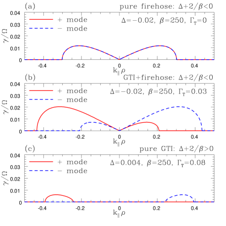
Figure 1: Growth rates of the firehose and gyrothermal instabilities (equation (24)) in three qualitatively different regimes: (a) pure firehose, $\Gamma_{T}=0$; (b) GTI combined with firehose, $\Delta+2/\beta<0$; (c) pure GTI, $\Delta+2/\beta>0$ (firehose stable). We have set $\delta=\Delta-2/\beta$, i.e., $p_{\perp e}-p_{\parallel e}=0$.

3.2 Gyrothermal instability

The situation becomes more complicated when the heat fluxes are not negligible. Let us assume, without loss of generality, that $\Gamma_{T}>0$ (otherwise, change the sign of the parallel spatial coordinate). There are two unstable intervals:

$$+~{}{\rm mode:} -\frac{4\left(\Gamma_{T}+\sqrt{\Lambda}\right)}{(1-\delta)^{2}}<k<-\frac{4\left(\Gamma_{T}-\sqrt{\Lambda}\right)}{(1-\delta)^{2}},$$ (29)

$$-~{}{\rm mode:} ~{}~{}\frac{4\left(\Gamma_{T}-\sqrt{\Lambda}\right)}{(1-\delta)^{2}}<k<\frac{4\left(\Gamma_{T}+\sqrt{\Lambda}\right)}{(1-\delta)^{2}}.$$ (30)

When $\Delta+2/\beta\leq 0$, these intervals intersect and contain $k=0$, otherwise they are disjoint (see figure 1b,c). Computing their peak growth rates and corresponding wavenumbers is straightforward. Here we consider two interesting limits.

When $\Gamma_{T}^{2}\gg|\Delta+2/\beta|$, we have, for the $+$ and $-$ modes respectively:

$$k_{\mathrm{p}}=\mp\frac{6\Gamma_{T}}{(1-\delta)^{2}},\quad\gamma_{\rm max}=\frac{3\sqrt{3}\,\Gamma_{T}^{2}}{|1-\delta|^{3}}.$$ (31)

We see that an instability is present that is driven purely by heat fluxes, even when the pressure anisotropy is neutralized by the tension force ($\Delta=-2/\beta$). This is the purest form of the gyrothermal instability (GTI), which, as far as we know, has not been previously reported in the literature. In the more general case when the pressure anisotropy is not negligible, the GTI operates in conjunction with the firehose. The condition (25) means that GTI can be operative even when $\Delta+2/\beta>0$, a regime in which the Alfvén waves have previously been believed to be stable.

The second important limit is the case when GTI is close to marginal stability, $\Lambda\to+0$ (we are assuming that $\Gamma_{T}^{2}$ is finite, so the firehose is stable in this limit). According to equations (29) and (30), the instability intervals in this limit shrink to the immediate vicinity of just two wavenumbers:

$$k_{\mathrm{p}}=\mp\frac{4\Gamma_{T}}{(1-\delta)^{2}}\left(1+\frac{\Lambda}{\Gamma_{T}^{2}}\right),\quad\gamma_{\rm max}=\frac{4\Gamma_{T}\sqrt{\Lambda}}{|1-\delta|^{3}},$$ (32)

where the upper sign is for the $+$ mode, the lower for the $-$ mode. This is a very different behaviour from the firehose, for which the interval of growing modes moves to ever longer wavelengths as marginal stability ($\Delta+2/\beta\to-0$) is approached (see equation (LABEL:eq:k0)), i.e., the firehose stops being a microscale instability in this limit. In contrast, the GTI always excites Alfvénic fluctuations at very short wavelengths.

Finally, we note that the assumption in our derivation that $\omega/\Omega\ll 1$ and $k_{\parallel}\rho\ll 1$ imposes constraints on the values of our dimensionless parameters that we are allowed to consider: $|\Delta+2/\beta|\ll 1$ for the firehose and $\Gamma_{T}\ll 1$ for the GTI. The expressions for maximum growth rates and corresponding wavenumbers derived above (equations (28), (31) and (32)) provide guidance on the relative smallness of all these quantities and, therefore, on the ordering schemes that can be pursued in weakly nonlinear theories (one example is the ordering adopted by Rosin et al. 2010).

4 Nonlinear evolution

Nonlinear theories of pressure-anisotropy-driven plasma instabilities are in their infancy, but most of them agree that the net result is to drive the anisotropies towards marginal stability thresholds (e.g., Shapiro & Shevchenko, 1964; Quest & Shapiro, 1996; Matteini et al., 2006; Schekochihin et al., 2008; Califano et al., 2008; Istomin et al., 2009; Rosin et al., 2010). Observational evidence from the solar wind strongly points in the same direction (Kasper, Lazarus & Gary, 2002; Hellinger et al., 2006; Matteini et al., 2007; Bale et al., 2009).

If we assume that this is what happens in the case of the firehose and gyrothermal instabilities, then the marginal state $\Lambda=0$ (see equation (25)) implies a certain relationship between the heat fluxes and the pressure anisotropy in the nonlinear regime. In order to find the way in which the system contrives to set up this relationship, we must first examine the physical mechanisms that determine $\Delta$, $q_{\perp}$ and $q_{\parallel}$.

Subtracting equation (4) from equation (3), we get

$$\frac{\mathrm{d}(p_{\perp}-p_{\parallel})}{\mathrm{d}t}=(p_{\perp}+2p_{\parallel})\frac{1}{B}\frac{\mathrm{d}B}{\mathrm{d}t}-(3p_{\parallel}-p_{\perp})\frac{1}{n}\frac{\mathrm{d}n}{\mathrm{d}t}$$ (33)

$$\quad\qquad-\,\mn@boldsymbol{\nabla}\cdot\left(\mn@boldsymbol{q}_{\perp}-\mn@boldsymbol{q}_{\parallel}\right)-3q_{\perp}\mn@boldsymbol{\nabla}\cdot\mn@boldsymbol{b}-3\nu(p_{\perp}-p_{\parallel}).$$

This tells us that there are three sources of pressure anisotropy: changing magnetic-field strength (changes in $p_{\perp}$ have to match changes in $B$ to maintain conservation of the first adiabatic invariant for each particle, $\mu=mv_{\perp}^{2}/2B$), compression/rarefaction, and heat fluxes.

If we assume for a moment that the collision rate is larger than the rate of change of all fields, then the differences between $p_{\perp}$ and $p_{\parallel}$ in equation (33) can be neglected everywhere except the collisional term and so the steady-state average pressure anisotropy satisfies

$$\Delta=\frac{1}{\nu}\Biggl{\{}\frac{1}{B}\frac{\mathrm{d}B}{\mathrm{d}t}-\frac{2}{3}\frac{1}{n}\frac{\mathrm{d}n}{\mathrm{d}t}-\frac{\mn@boldsymbol{\nabla}\cdot\left[\mn@boldsymbol{b}(q_{\perp}-q_{\parallel})\right]+3q_{\perp}\mn@boldsymbol{\nabla}\cdot\mn@boldsymbol{b}}{3p_{\parallel}}\Biggr{\}}.$$

(34)

Note that if we use equations (12) and (1) (neglecting FLR terms in the induction equation) to express the rates of change of $B$ and $n$ in the right-hand side of equation (34), the first two terms are the Braginskii (1965) parallel viscous stress. The last term is the heat-flux correction to it introduced by Mikhailovskii & Tsypin (1971, 1984) for subsonic flows. Under the same assumption of high collisionality, the heat fluxes are

$$q_{\perp}=\frac{1}{3}\,q_{\parallel}=-\frac{1}{2}\,n\,\frac{v_{\mathrm{th}}^{2}}{\nu}\,\mn@boldsymbol{b}\cdot\mn@boldsymbol{\nabla}T,$$ (35)

where $T=p/n$ and $p=(2/3)p_{\perp}+(1/3)p_{\parallel}$.

As we showed in section 3, the slow macroscale motions that produce this $\Delta$ and these heat fluxes are unstable to microscale perturbations, in particular, the Alfvénic ones excited by the firehose/GTI. Schekochihin et al. (2008) showed that the way a sea of small-scale Alfvénic fluctuations can change a large-scale driven anisotropy is by growing secularly with time and thus producing a finite change in the average field strength:

$$\overline{\frac{1}{B}\frac{\mathrm{d}B}{\mathrm{d}t}}=\frac{1}{B_{0}}\frac{\mathrm{d}B_{0}}{\mathrm{d}t}+\frac{1}{2}\frac{\partial\overline{|\delta\mn@boldsymbol{b}|^{2}}}{\partial t},$$ (36)

where the overbar denotes a small-scale average, $B_{0}$ is the slowly changing macroscale field and $\delta\mn@boldsymbol{b}=\delta\mn@boldsymbol{B}_{\perp}/B_{0}$ is the fast microscale Alfvénic perturbation of it. Let us replace the magnetic term in equation (34) with its average given by equation (36). Even though the fluctuation amplitude is small, the nonlinear feedback will produce a finite contribution to $\Delta$ if the fluctuation energy grows secularly, $\overline{|\delta\mn@boldsymbol{b}|^{2}}\sim\gamma_{0}t$, where $\gamma_{0}$ is the typical rate of change of $B_{0}$. There does not appear to be any other way for the small Alfvénic fluctuations to affect the average macroscopic pressure anisotropy or heat fluxes.

In the case of the pure firehose instability (no heat fluxes), the nonlinear feedback described above cancels the negative pressure anisotropy that triggered the firehose and pushes the system towards $\Delta+2/\beta\to-0$. If heat fluxes are present, the marginal state of the GTI requires $\Delta+2/\beta>0$ ($\Lambda\to+0$; see equation (25)). This can still be achieved by secularly growing Alfvénic fluctuations (which, unlike for the firehose, now have a definite scale unaffected by the pressure anisotropy; this is explored further in Rosin et al. 2010).

A remarkable consequence of this predicted tendency for a system to develop positive pressure anisotropy to cancel the destabilizing effect of heat fluxes is that instabilities associated with $\Delta>0$ (e.g., mirror) could perhaps be triggered as secondary instabilities of the saturated state of the GTI. One might imagine a sea of Alfvénic fluctuations attempting to neutralize the GTI and exciting unstable mirror modes — this is feasible if the pressure anisotropy corresponding to the marginal state of the GTI exceeds the mirror stability threshold: $\Delta\simeq 2\Gamma_{T}^{2}-2/\beta>1/\beta$, i.e., $\Gamma_{T}^{2}>3/2\beta$. The mirror mode near its threshold $\Delta-1/\beta\to+0$ is polarized as a highly oblique slow wave: it has $\delta u_{\parallel}$ and $\delta B_{\parallel}$ with $k_{\parallel}\rho\sim\Delta-1/\beta\ll k_{\perp}\rho\sim(\Delta-1/\beta)^{1/2}$ (see, e.g., Hellinger, 2007). This suggests a three-scale system: a macroscale equilibrium, the microscale Alfvénic foam with $k_{\parallel}\rho\sim\Gamma_{T}\sim 1/\sqrt{\beta}$ (see equation (32)) driven by the GTI and producing an average pressure anisotropy, and a mesoscale near-threshold mirror turbulence driven by that anisotropy and, because of scale separation, probably otherwise disconnected from the Alfvénic modes. Finding out how they all coexist and how the mirror saturates requires a systematic kinetic calculation, which will be attempted elsewhere.

Finally, as an alternative to the above considerations, we should perhaps mention the possibility of strong nonlinear distortions of the magnetic field ($\delta\mn@boldsymbol{b}\sim 1$) that could reorient the field so as to minimize the parallel ion temperature gradient and thus switch off or weaken the GTI — on large scales, such behaviour has been observed in simulations of another, macroscale, instability driven by the parallel (electron) heat flux and buoyancy force, called the heat-flux-buoyancy instability, or HBI (Sharma et al., 2009; Parrish et al., 2009; Bogdanović et al., 2009).

5 Physical and astrophysical considerations

5.1 Physical conclusions

The main physical conclusion is that parallel heat fluxes can directly drive microscale instabilities in magnetized astrophysical plasmas. This can happen in two ways.

First, as follows from equation (33), plasma pressure anisotropy can be driven by heat fluxes, so firehose, mirror and the rest of the microinstabilities due to $p_{\perp}-p_{\parallel}\neq 0$ can be triggered not just by plasma motions, but also by parallel temperature gradients. Although perhaps not much discussed explicitly, this instability mechanism is not particularly surprising and it is implicitly present in the existing analytical and numerical models based on CGL equations with heat fluxes (e.g., Snyder et al., 1997; Quataert et al., 2002; Sharma et al., 2006, 2007).

A more interesting and, we believe, novel instability mechanism is the destabilization of the Alfvénic perturbations by the ion parallel heat fluxes via the FLR effects in the plasma pressure tensor — we call this the gyrothermal instability (GTI). When the firehose is unstable, the GTI can substantially modify (increase) its growth rate, but more importantly, the GTI persists even when the firehose is stable, so the firehose marginal stability condition has to be replaced by the GTI marginal stability condition involving both the pressure anisotropy and the ion heat flux (equation (25)).

The GTI is distinct from the two other instabilities associated with the presence of temperature gradients and recently explored in astrophysical contexts — the MTI (Balbus, 2000; Parrish & Stone, 2007; Parrish et al., 2008) and the HBI (Quataert, 2008; Sharma et al., 2009; Parrish et al., 2009; Bogdanović et al., 2009; Ruszkowski & Oh, 2009). The latter are driven by buoyancy and are essentially macroscale fluid instabilities, like MRI (Balbus & Hawley, 1998) or MVI (Balbus, 2004). They are also much slower than the GTI, which is a microscale plasma instability belonging to the same class as the firehose, with peak growth rate a fraction of the cyclotron frequency. Since such an instability can be triggered by the presence of a heat flux, one might wonder whether in the same way that large-scale pressure anisotropy could be conjectured always to be determined by the marginal stability conditions of the microinstabilities (Sharma et al., 2006, 2007; Schekochihin & Cowley, 2006; Lyutikov, 2007; Kunz et al., 2010), the heat fluxes as well should be constrained by the marginal stability conditions of the GTI and, perhaps, other such instabilities. We stress, however, that, whereas this might be a reasonable interim course of action, it by no means excuses us from the task of finding out how GTI and the rest of the instabilities behave and saturate on the microphysical level (see discussion in section 4).

5.2 An astrophysical example: galaxy clusters

A detailed development of applications to concrete astrophysical systems falls outside the scope of this paper (see, e.g., Kunz et al., 2010). However, it is, perhaps, illuminating to provide a few estimates of the role the GTI might play in cool cores of relaxed galaxy clusters, a good example of a real astrophysical plasma for which a sufficient amount of observational evidence exists to enable a quantitative discussion of the multiscale dynamics.

5.2.1 Three-scale dynamics

The conditions in the cluster cores are believed to be controlled by a balance between the radiative cooling and a reheating due perhaps to electron heat conduction from the bulk of the cluster and perhaps also to the turbulence excited by the active galactic nuclei (e.g., Binney, 2003; Dennis & Chandran, 2005; Peterson & Fabian, 2006; McNamara & Nulsen, 2007; Guo et al., 2008; Ruszkowski & Oh, 2009, and references therein). The plasma in the cores has the electron density $n_{e}$ in the range $10^{-2}$ to $10^{-1}$ cm^-3 at the radial distance of $r\sim 10$ kpc from the centre and about a factor of 10 less at the edge of the core at $r\sim 100$ kpc. The ion density is the same for a hydrogen plasma. The electron temperature $T_{e}$ is measured reasonably precisely and is of the order of a few keV, rising by about a factor of 2 or 3 from $r\sim 10$ kpc to $100$ kpc (e.g., David et al., 2001; Vikhlinin et al., 2005; Fabian et al., 2006; Leccardi & Molendi, 2008; Sanders et al., 2010a, b). The ion temperature is not measured, but the ion-electron temperature equilibration turns out to be quite fast compared to all other relevant dynamics, so $T_{i}\sim T_{e}$ can reasonably be assumed. The unsolved macroscale problem is why the temperature does not drop lower in the centre — simple estimates suggest that the system should be vulnerable to a collapse onto the centre precipitated by the radiative cooling on a characteristic time scale of about 1 Gyr.

This is where turbulent heat conduction and turbulent heating are invoked as mechanisms that prevent the cooling catastrophe. The outer scale $L$ of turbulent motions is believed to be between a few and a few tens of kpc, with corresponding velocities $U$ of a few hundred ${\rm km\,s}^{-1}$ (Enßlin & Vogt, 2006; Sanders et al., 2010b). The turbulent motions lead to fluctuations in the magnetic-field strength and so excite pressure anisotropies, given by equation (34). Equation (12) tells us that the typical rate of change of the field is comparable to the typical rate of strain $\sim(U/L)\mathrm{Re}^{1/2}$, where $\mathrm{Re}\sim UL\nu/v_{\mathrm{th}}^{2}$ is the Reynolds number (the maximum rate of strain that can affect the magnetic-field strength is at the viscous scale set by the parallel viscosity; see Schekochihin & Cowley 2006 for a detailed explanation). Thus, we estimate the pressure anisotropy as follows:

$$\Delta \sim \frac{1}{\nu}\frac{U}{L}\,\mathrm{Re}^{1/2}\sim\left(\frac{1}{\nu}\frac{U}{L}\right)^{1/2}\frac{U}{v_{\mathrm{th}}}$$ (37)

$$\sim 0.007\left(\frac{n_{e}}{0.01\,\rm{cm}^{-3}}\right)^{-1/2}\left(\frac{T_{i}}{1\,\rm{keV}}\right)^{1/4}$$

$$\times\left(\frac{U}{100\,\rm{km\,s}^{-1}}\right)^{3/2}\left(\frac{L}{10\,\rm{kpc}}\right)^{-1/2},$$

where $\nu$ is the ion collision rate. In view of the instability condition (25), whether this anisotropy will trigger plasma microinstabilities is decided by comparing it with

$$\frac{2}{\beta}=0.005\left(\frac{B}{1\,\mu\rm{G}}\right)^{2}\left(\frac{n_{e}}{0.01\,\rm{cm}^{-3}}\right)^{-1}\left(\frac{T_{i}}{1\,\rm{keV}}\right)^{-1}.$$ (38)

The two numbers are remarkably close (obviously, only orders of magnitude matter here, given all the uncertainties). Thus the intracluster plasma teeters at the brink of marginal stability. In the unstable state, at the reference values $B=1\,\mu$G and $T_{i}=1\,$keV, the firehose (or GTI) will have growth times and peak-growth scales

$$\gamma_{\rm max}^{-1}\sim\left(\Delta\Omega_{i}\right)^{-1}\sim 2\cdot 10^{4}\,\rm{s}\simeq 6\,\rm{hr},$$ (39)

$$k_{\mathrm{p}}^{-1}\sim\Delta^{-1/2}\rho_{i}\sim 700,000\,\rm{km}\simeq 20\,\rm{npc}$$ (40)

(see section 3). These are microscopic scales compared both to global cluster dynamics and intracluster turbulence. The implication is that the plasma instabilities should saturate and presumably contrive to return the intracluster medium to marginal stability instantaneously fast via an observationally invisible sea of nanoparsec-scale magnetic fluctuations.

Thus, a cluster core is a “three-scale system”: global equilibrium profiles ($10^{2}$ kpc, $10^{0}$ Gyr) and turbulence ($10^{1}$ kpc, $10^{1}$ Myr) constitute the macroscale magnetofluid dynamics of the intracluster medium, subject to transport properties controlled by “nanoscales” ($10^{1}$ npc, $10^{1}$ hr), where plasma microinstabilities are excited. Their nonlinear behaviour sets the pressure anisotropy and probably also the heat fluxes. The pressure anisotropy determines the effective viscosity of the plasma and, therefore the heating rate; the heat fluxes determine the effective thermal conductivity — thus, neither the turbulence nor the global dynamics (e.g., temperature profiles for the cooling-core problem) can be computed correctly without a good theory or, at least, a good model prescription, for the effect of the microinstabilities on the macroscale dynamics. A similar three-scale situation arises in most other weakly collisional cosmic plasmas: e.g., accretion flows, solar wind, etc.

5.2.2 Temperature fluctuations

As we have shown in this paper, ion temperature gradients, including ones due to temperature fluctuations, if they are there and if the associated parallel heat fluxes are large enough, will excite microinstabilities. The estimates of $\gamma_{\rm max}$ and $k_{\mathrm{p}}$ in section 5.2.1 still hold, by order of magnitude, for the GTI, so the instability is extremely fast and one should expect to find plasma close to the marginal state. We may estimate (crudely), the minimum parallel temperature length scale allowed by the instability condition (25) by requiring $\Gamma_{T}^{2}\lesssim 2/\beta$ for stability and using equation (35) for the heat fluxes:

$$l_{T}\gtrsim 0.3\left(\frac{n_{e}}{0.01\,\rm{cm}^{-3}}\right)^{-1/2}\left(\frac{T_{i}}{1\,\rm{keV}}\right)^{5/2}\left(\frac{B}{1\,\mu\rm{G}}\right)^{-1}\rm{kpc},$$ (41)

where $l_{T}^{-1}=\mn@boldsymbol{b}\cdot\mn@boldsymbol{\nabla}\ln T$ is the temperature scale. Note the very strong temperature dependence of this lower bound: thus, deep in the cool cores, the estimate above gives kiloparsec-scale temperature fluctuations, rising to tens and even hundreds of kpc at larger distances from the centre.

Interestingly, temperature fluctuations on 1 to 10 kpc scales have been detected in cool-core clusters (Simionescu et al., 2001; Fabian et al., 2006; Sanders et al., 2010a) while in the bulk of the cluster gas and in non-cool-core (radio-halo) clusters, the scales appear to be larger, around 100 kpc (Markevitch et al., 2003; Million & Allen, 2009). Thus, we again find the observed physical conditions intriguingly close to the marginal stability conditions set by plasma microphysics. Nevertheless, we would like to conclude on a cautious note: whether the plasma contrives to satisfy the lower bound (41) by smoothing the temperature gradients or by aligning them carefully across the magnetic field remains unclear and underscores the need for a detailed theory of the nonlinear saturation of the GTI and other plasma microinstabilities. Observationally, it would be fascinating to see if any evidence can be obtained of correlations between the magnetic field direction and temperature fluctuations — presumably not an impossible task if one combines radio observations of polarized synchrotron emission and X-ray temperature maps (cf. Taylor et al., 2006).

Appendix A Plasma pressure tensor

We start with the general kinetic equation for the distribution function of a plasma species:

$$\frac{\mathrm{d}f}{\mathrm{d}t}+\mn@boldsymbol{v}\cdot\mn@boldsymbol{\nabla}f+\left(\mn@boldsymbol{a}+\frac{e}{m}\frac{\mn@boldsymbol{v}\times\mn@boldsymbol{B}}{c}-\mn@boldsymbol{v}\cdot\mn@boldsymbol{\nabla}\mn@boldsymbol{u}\right)\!\cdot\!\frac{\partial f}{\partial\mn@boldsymbol{v}}=C[f],$$ (42)

where $e$ is the particle charge, $c$ the speed of light, $\mn@boldsymbol{a}=(e/m)(\mn@boldsymbol{E}+\mn@boldsymbol{u}\times\mn@boldsymbol{B}/c)-\mathrm{d}\mn@boldsymbol{u}/\mathrm{d}t$ and $C[f]$ is the collision integral. The flow velocity $\mn@boldsymbol{u}$ appears in the kinetic equation because $\mn@boldsymbol{v}$ is the peculiar velocity. Since $(e/mc)(\mn@boldsymbol{v}\times\mn@boldsymbol{B})\cdot\partial f/\partial\mn@boldsymbol{v}=-\Omega\partial f/\partial\vartheta$, where $\Omega$ is the Larmor frequency and $\vartheta$ is the phase angle of the particle’s gyration around the magnetic-field line, equation (42) can be rewritten as follows

$$\Omega\,\frac{\partial f}{\partial\vartheta}=\frac{\mathrm{d}f}{\mathrm{d}t}+\mn@boldsymbol{v}\cdot\mn@boldsymbol{\nabla}f+\left(\mn@boldsymbol{a}-\mn@boldsymbol{v}\cdot\mn@boldsymbol{\nabla}\mn@boldsymbol{u}\right)\cdot\frac{\partial f}{\partial\mn@boldsymbol{v}}-C[f].$$ (43)

We can now express the plasma pressure tensor $\textbf{{P}}=m\int\mathrm{d}^{3}\mn@boldsymbol{v}\,\mn@boldsymbol{v}\mn@boldsymbol{v}f$ using the following identity

$$\mn@boldsymbol{v}\mn@boldsymbol{v} = \frac{v_{\perp}^{2}}{2}\left(\textbf{{I}}-\mn@boldsymbol{b}\mn@boldsymbol{b}\right)+v_{\parallel}^{2}\mn@boldsymbol{b}\mn@boldsymbol{b}+\frac{\partial\textbf{{T}}}{\partial\vartheta},$$ (44)

T $$= \left(v_{\parallel}\mn@boldsymbol{b}+\frac{\mn@boldsymbol{v}_{\perp}}{4}\right)\left(\mn@boldsymbol{v}_{\perp}\times\mn@boldsymbol{b}\right)+\left(\mn@boldsymbol{v}_{\perp}\times\mn@boldsymbol{b}\right)\left(v_{\parallel}\mn@boldsymbol{b}+\frac{\mn@boldsymbol{v}_{\perp}}{4}\right),$$

or, in index notation, $T_{ij}=(1/4)M_{ijkl}v_{k}v_{l}$, where

$$M_{ijkl}=\left(\delta_{ik}+3b_{i}b_{k}\right)\epsilon_{jln}b_{n}+\epsilon_{iln}b_{n}\left(\delta_{jk}+3b_{j}b_{k}\right).$$ (45)

Therefore, after integration by parts with respect to $\vartheta$,

$$P_{ij}=p_{\perp}\delta_{ij}-(p_{\perp}-p_{\parallel})b_{i}b_{j}-\frac{M_{ijkl}}{4}\!\int\!\mathrm{d}^{3}\mn@boldsymbol{v}\,mv_{k}v_{l}\,\frac{\partial f}{\partial\vartheta}.$$ (46)

We now substitute equation (43) into the above expression and notice that $\int\mathrm{d}^{3}\mn@boldsymbol{v}\,\mn@boldsymbol{v}\mn@boldsymbol{v}\,\mn@boldsymbol{a}\cdot\partial f/\partial\mn@boldsymbol{v}=0$ after integration by parts and using the fact that $\int\mathrm{d}^{3}\mn@boldsymbol{v}\,\mn@boldsymbol{v}f=0$ by definition of peculiar velocity. We get, therefore,

$$P_{ij} = p_{\perp}\delta_{ij}-(p_{\perp}-p_{\parallel})b_{i}b_{j}-\frac{M_{ijkl}}{4\Omega}\biggl{[}\frac{\mathrm{d}P_{kl}}{\mathrm{d}t}+\nabla_{m}Q_{mkl}\biggr{.}$$ (47)

$$+\biggl{.}\bigl{(}\delta_{mn}P_{kl}+\delta_{kn}P_{ml}+\delta_{ln}P_{mk}\bigr{)}\nabla_{m}u_{n}-C_{kl}\biggr{]},$$

where $C_{kl}=m\int\mathrm{d}^{3}\mn@boldsymbol{v}\,v_{k}v_{l}C[f]$ and we have introduced the heat flux tensor $Q_{mkl}=m\int\mathrm{d}^{3}\mn@boldsymbol{v}\,v_{m}v_{k}v_{l}f$.

So far we have made no approximations. As promised in section 2, we now calculate all terms in equation (47) assuming that we can use a gyrotropic (independent of $\vartheta$) distribution function. This amounts to setting up a perturbation theory in which to lowest order, equation (43) gives a gyrotropic equilibrium distribution, $\Omega\partial f_{0}/\partial\vartheta=0$, and at the next order we have $\Omega\partial\delta f/\partial\vartheta=\dots$, where only $f_{0}$ appears in the right-hand side. The assumptions we need to achieve such an expansion are $\omega/\Omega\ll 1$ and $k\rho\ll 1$ for all quantities involved.

Since $f_{0}$ is gyrotropic, we may gyroaverage $\left<v_{k}v_{l}\right>=(1/2\pi)\int\mathrm{d}\vartheta\,v_{k}v_{l}=(v_{\perp}^{2}/2)(\delta_{kl}-b_{k}b_{l})+v_{\parallel}^{2}b_{k}b_{l}$ inside all the velocity integrals in the square brackets in equation (47), so we get

$$M_{ijkl}P_{kl}\nabla_{m}u_{m}=M_{ijkl}C_{kl}=0,$$ (48)

$$M_{ijkl}P_{ml}\nabla_{m}u_{k}=$$ (49)

$$-p_{\perp}\left[\mn@boldsymbol{b}\times(\mn@boldsymbol{\nabla}\mn@boldsymbol{u})\cdot\left(\textbf{{I}}+3\mn@boldsymbol{b}\mn@boldsymbol{b}\right)-\left(\textbf{{I}}+3\mn@boldsymbol{b}\mn@boldsymbol{b}\right)\cdot(\mn@boldsymbol{\nabla}\mn@boldsymbol{u})^{T}\times\mn@boldsymbol{b}\right],$$

$$M_{ijkl}P_{mk}\nabla_{m}u_{l}=$$ (50)

$$-p_{\perp}\left[\mn@boldsymbol{b}\times(\mn@boldsymbol{\nabla}\mn@boldsymbol{u})^{T}\cdot\left(\textbf{{I}}+3\mn@boldsymbol{b}\mn@boldsymbol{b}\right)-\left(\textbf{{I}}+3\mn@boldsymbol{b}\mn@boldsymbol{b}\right)\cdot(\mn@boldsymbol{\nabla}\mn@boldsymbol{u})\times\mn@boldsymbol{b}\right]$$

$$-4(p_{\perp}-p_{\parallel})\bigl{[}\mn@boldsymbol{b}\left(\mn@boldsymbol{b}\cdot\mn@boldsymbol{\nabla}\mn@boldsymbol{u}\times\mn@boldsymbol{b}\right)+\left(\mn@boldsymbol{b}\cdot\mn@boldsymbol{\nabla}\mn@boldsymbol{u}\times\mn@boldsymbol{b}\right)\mn@boldsymbol{b}\bigr{]},$$

$$M_{ijkl}\frac{\mathrm{d}P_{kl}}{\mathrm{d}t}=-4(p_{\perp}-p_{\parallel})\left(\mn@boldsymbol{b}\,\frac{\mathrm{d}\mn@boldsymbol{b}}{\mathrm{d}t}\times\mn@boldsymbol{b}+\frac{\mathrm{d}\mn@boldsymbol{b}}{\mathrm{d}t}\times\mn@boldsymbol{b}\,\mn@boldsymbol{b}\right).$$ (51)

Similarly gyroaveraging $\left<v_{m}v_{k}v_{l}\right>$ in the heat flux integral, $Q_{mkl}=q_{\perp}\left(b_{m}\delta_{kl}+\delta_{mk}b_{l}+\delta_{ml}b_{k}\right)-(3q_{\perp}-q_{\parallel})b_{m}b_{k}b_{l}$. Therefore,

$$M_{ijkl}\nabla_{m}Q_{mkl}=\left(\textbf{{I}}+3\mn@boldsymbol{b}\mn@boldsymbol{b}\right)\cdot\bigl{[}\mn@boldsymbol{\nabla}\mn@boldsymbol{q}_{\perp}+(\mn@boldsymbol{\nabla}\mn@boldsymbol{q}_{\perp})^{T}\bigr{]}\times\mn@boldsymbol{b}$$ (52)

$$-\,\mn@boldsymbol{b}\times\bigl{[}\mn@boldsymbol{\nabla}\mn@boldsymbol{q}_{\perp}+(\mn@boldsymbol{\nabla}\mn@boldsymbol{q}_{\perp})^{T}\bigr{]}\cdot\left(\textbf{{I}}+3\mn@boldsymbol{b}\mn@boldsymbol{b}\right)$$

$$-\,4(3q_{\perp}-q_{\parallel})\bigl{[}\mn@boldsymbol{b}\left(\mn@boldsymbol{b}\cdot\mn@boldsymbol{\nabla}\mn@boldsymbol{b}\times\mn@boldsymbol{b}\right)+\left(\mn@boldsymbol{b}\cdot\mn@boldsymbol{\nabla}\mn@boldsymbol{b}\times\mn@boldsymbol{b}\right)\mn@boldsymbol{b}\bigr{]}.$$

Assembling equations (48–LABEL:eq:Mdt) and (52) together in equation (47), we obtain equations (5–8).

Appendix B CGL equations

In order to derive equations (3) and (4), we average equation (43) over the gyroangles, $(1/2\pi)\int\mathrm{d}\vartheta$, which eliminates the left-hand side. In the remainder, we assume that the lowest-order distribution function is gyrotropic and so can be written as $f=f(t,\mn@boldsymbol{r},v,v_{\parallel})$. The time and spatial derivatives in equation (43) are taken at constant $\mn@boldsymbol{v}$, so, in order for the gyroaverage to commute with them, they have to be transformed into derivatives at constant $v$ and $v_{\parallel}$, a nontrivial step because $v_{\parallel}=\mn@boldsymbol{v}\cdot\mn@boldsymbol{b}(t,\mn@boldsymbol{r})$:

$$\left(\frac{\mathrm{d}f}{\mathrm{d}t}\right)_{\mn@boldsymbol{v}} = \left(\frac{\mathrm{d}f}{\mathrm{d}t}\right)_{v,v_{\parallel}}+\frac{\mathrm{d}\mn@boldsymbol{b}}{\mathrm{d}t}\cdot\mn@boldsymbol{v}\left(\frac{\partial f}{\partial v_{\parallel}}\right)_{v},$$ (53)

$$\left(\mn@boldsymbol{\nabla}f\right)_{\mn@boldsymbol{v}} = \left(\mn@boldsymbol{\nabla}f\right)_{v,v_{\parallel}}+\left(\mn@boldsymbol{\nabla}\mn@boldsymbol{b}\right)\cdot\mn@boldsymbol{v}\left(\frac{\partial f}{\partial v_{\parallel}}\right)_{v}.$$ (54)

Using these formulae and also $\partial f/\partial\mn@boldsymbol{v}=(\mn@boldsymbol{v}/v)\partial f/\partial v+\mn@boldsymbol{b}\partial f/\partial v_{\parallel}$ and $\left<\mn@boldsymbol{v}\right>=v_{\parallel}\mn@boldsymbol{b}$, $\left<\mn@boldsymbol{v}\mn@boldsymbol{v}\right>=(v_{\perp}^{2}/2)(\textbf{{I}}-\mn@boldsymbol{b}\mn@boldsymbol{b})+v_{\parallel}^{2}\mn@boldsymbol{b}\mn@boldsymbol{b}$, we find that the gyroaveraged equation (43) is

$$\frac{\mathrm{d}f}{\mathrm{d}t}+v_{\parallel}\mn@boldsymbol{b}\cdot\mn@boldsymbol{\nabla}f+\frac{v_{\perp}^{2}}{2}\left(\mn@boldsymbol{\nabla}\cdot\mn@boldsymbol{b}\right)\frac{\partial f}{\partial v_{\parallel}}+\mn@boldsymbol{a}\cdot\mn@boldsymbol{b}\left(\frac{v_{\parallel}}{v}\frac{\partial f}{\partial v}+\frac{\partial f}{\partial v_{\parallel}}\right)$$ (55)

$$+\left(\mn@boldsymbol{b}\mn@boldsymbol{b}:\mn@boldsymbol{\nabla}\mn@boldsymbol{u}\right)\left[\left(\frac{v_{\perp}^{2}}{2}-v_{\parallel}^{2}\right)\frac{1}{v}\frac{\partial f}{\partial v}-v_{\parallel}\frac{\partial f}{\partial v_{\parallel}}\right]$$

$$-\left(\mn@boldsymbol{\nabla}\cdot\mn@boldsymbol{u}\right)\frac{v_{\perp}^{2}}{2}\frac{1}{v}\frac{\partial f}{\partial v}=C[f].$$

Changing variables from $(v,v_{\parallel})$ to $(v_{\perp},v_{\parallel})$ or $(\mu,v_{\parallel})$, where $\mu=v_{\perp}^{2}/2B$, transforms this equation into forms that are perhaps more familiar from the well-known Kinetic MHD approximation (Kulsrud, 1983).

Equations (3) and (4) are obtained by taking the $v_{\perp}^{2}/2$ and $v_{\parallel}^{2}$ moments of equation (55) and integrating by parts wherever opportune. The collisional relaxation terms are easiest to calculate with a simplified collisional operator, e.g., Krook (Snyder et al., 1997) or Lorentz (Rosin et al., 2010). To complete the picture, it may be useful to mention here that in some cases, especially when the pressure anisotropy $p_{\perp}-p_{\parallel}$ is small compared to the pressures themselves, it is convenient to replace equations (3) and (4) by equation (33) determining the evolution of $p_{\perp}-p_{\parallel}$ and an equation for the total pressure $p=(2/3)p_{\perp}+(1/3)p_{\parallel}$ or temperature $T$ defined by $p=nT$. Using equations (3) and (4), we get

$$\frac{3}{2}\,n\,\frac{\mathrm{d}T}{\mathrm{d}t}=p\,\frac{1}{n}\frac{\mathrm{d}n}{\mathrm{d}t}+(p_{\perp}-p_{\parallel})\left(\frac{1}{B}\frac{\mathrm{d}B}{\mathrm{d}t}-\frac{2}{3}\frac{1}{n}\frac{\mathrm{d}n}{\mathrm{d}t}\right)-\mn@boldsymbol{\nabla}\cdot\mn@boldsymbol{q},$$ (56)

where $\mn@boldsymbol{q}=\mn@boldsymbol{q}_{\perp}+\mn@boldsymbol{q}_{\parallel}/2$. The first term is compressional heating, the second viscous heating and the third the heat flux. While the same-species collisions do not affect the evolution of temperature (because of the energy and particle conservation), we do have to add to the above equation a temperature equilibration term, $-(3/2)n_{i}\nu_{ie}(T_{i}-T_{e})$ for ions and negative of the same for electrons, where $\nu_{ie}$ is the ion-electron collision frequency (the ion-electron temperature equilibration terms were omitted in equations (3) and (4) because the relaxation of the pressure anisotropy was the dominant collisional effect there). In situations where radiative cooling is important (as in the case of galaxy clusters discussed in section 5.2), the electron temperature equation should also have a cooling term, $-n_{i}n_{e}\Lambda(T_{e})$, where $\Lambda$ is the cooling function (e.g., Tozzi & Norman, 2001).

Note that, in principle, since we kept the FLR terms in the pressure tensor, we should also have kept FLR corrections in the CGL equations. These arise from the FLR contribution to the heat flux — in the collisional limit, it is the usual diamagnetic heat flux $\delta\mn@boldsymbol{q}=(5nv_{\mathrm{th}}^{2}/4\Omega)\,\mn@boldsymbol{b}\times\mn@boldsymbol{\nabla}T$ (see Braginskii, 1965). While the unperturbed part of these FLR terms is small compared to other macroscale terms, their perturbed part is comparable to the perturbed gyroviscous stress terms ($\mn@boldsymbol{k}\cdot\delta\textbf{{G}}$ in equation (14)). In equation (14), the diamagnetic heat-flux terms are part of the perturbed pressures $\delta p_{\perp}$ and $\delta p_{\parallel}$. Since the instabilities we study in this paper are Alfvénically polarized and so are indifferent to pressure perturbations, we do not need to calculate the diamagnetic heat fluxes and, therefore, omit them.

Appendix C Flux freezing

The non-MHD terms in equation (12) will still preserve the magnetic-field topology if the electric field can be expressed in the form $\mn@boldsymbol{E}=-\mn@boldsymbol{u}_{\rm eff}\times\mn@boldsymbol{B}/c+\mn@boldsymbol{\nabla}\chi$, where $\chi$ is an arbitrary scalar function and $\mn@boldsymbol{u}_{\rm eff}$ is some effective velocity field into which the flux will be frozen. Consider equation (11). It is not hard to show that the electron pressure term is

$$\mn@boldsymbol{\nabla}\cdot\textbf{{P}}_{e}=\mn@boldsymbol{\nabla}p_{\perp e}-\mn@boldsymbol{\nabla}\cdot\left[\mn@boldsymbol{b}\mn@boldsymbol{b}(p_{\perp e}-p_{\parallel e})\right]$$ (57)

$$=\mn@boldsymbol{\nabla}_{\perp}(p_{\perp e}-p_{\parallel e})-(p_{\perp e}-p_{\parallel e})\left(\frac{\mn@boldsymbol{\nabla}_{\perp}B}{B}+\mn@boldsymbol{b}\cdot\mn@boldsymbol{\nabla}\mn@boldsymbol{b}\right)$$

$$\hbox to0.0pt{$\displaystyle+\mn@boldsymbol{\nabla}p_{\parallel e}+(p_{\perp e}-p_{\parallel e})\,\frac{\mn@boldsymbol{\nabla}B}{B}$\hss},$$

where $\mn@boldsymbol{\nabla}_{\perp}=(\textbf{{I}}-\mn@boldsymbol{b}\mn@boldsymbol{b})\cdot\mn@boldsymbol{\nabla}$ and we have used $\mn@boldsymbol{\nabla}\cdot\mn@boldsymbol{b}=-\mn@boldsymbol{b}\cdot\mn@boldsymbol{\nabla}B/B$. Since the first two terms are perpendicular to $\mn@boldsymbol{B}$, they can be represented as a vector product of some effective vector field with $\mn@boldsymbol{B}$. Therefore, introducing

$$\mn@boldsymbol{u}_{\rm eff} = \mn@boldsymbol{u}_{e}-\frac{c}{en_{e}B^{2}}\Bigl{[}\mn@boldsymbol{\nabla}_{\perp}(p_{\perp e}-p_{\parallel e})\Bigr{.}$$ (58)

$$-\Bigl{.}(p_{\perp e}-p_{\parallel e})\left(\frac{\mn@boldsymbol{\nabla}_{\perp}B}{B}+\mn@boldsymbol{b}\cdot\mn@boldsymbol{\nabla}\mn@boldsymbol{b}\right)\Bigr{]}\times\mn@boldsymbol{B},$$

where $\mn@boldsymbol{u}_{e}=\mn@boldsymbol{u}-(c/4\pi en_{e})\mn@boldsymbol{\nabla}\times\mn@boldsymbol{B}$, we find from equation (11)

$$\mn@boldsymbol{E}=-\frac{\mn@boldsymbol{u}_{\rm eff}\times\mn@boldsymbol{B}}{c}-\frac{\mn@boldsymbol{\nabla}p_{\parallel e}}{en_{e}}-\frac{p_{\perp e}-p_{\parallel e}}{en_{e}}\frac{\mn@boldsymbol{\nabla}B}{B}.$$ (59)

With this electric field, Faraday’s law (10) becomes

$$\frac{\partial\mn@boldsymbol{B}}{\partial t} = \mn@boldsymbol{\nabla}\times(\mn@boldsymbol{u}_{\rm eff}\times\mn@boldsymbol{B})-\frac{c\mn@boldsymbol{\nabla}n_{e}\times\mn@boldsymbol{\nabla}p_{\parallel e}}{en_{e}^{2}}$$ (60)

$$+\left(c\mn@boldsymbol{\nabla}\frac{p_{\perp e}-p_{\parallel e}}{en_{e}}\right)\times\frac{\mn@boldsymbol{\nabla}B}{B},$$

which is an equivalent form of equation (12). Thus, the magnetic field is frozen into the effective velocity field $\mn@boldsymbol{u}_{\rm eff}$ except for two effects. The first of the two non-flux-conserving terms in equation (60) is the well-known Biermann (1950) battery (believed to be one of the mechanisms responsible for seeding the cosmic plasma with the initial magnetic fluctuations, subsequently amplified by turbulent dynamo; see Kulsrud et al. 1997); the second is an effect due to the electron pressure anisotropy. While it is not a battery in the sense of producing magnetic field from a zero initial condition (plasma is unmagnetized when $B=0$, so there is no pressure anisotropy), it is independent of the field strength and, therefore, can act as a source term.

The flux unfreezing effect due to the electron pressure anisotropy is small except at very small scales. If we use equation (33) to estimate $p_{\perp e}-p_{\parallel e}\sim(n_{e}T_{e}/\nu_{ei})(1/B)\mathrm{d}B/\mathrm{d}t$, we find, very roughly, that the flux conservation is significantly violated only if the scale of variation of $T_{e}$ and $B$ perpendicular to $\mn@boldsymbol{B}$ is $l_{\perp}\lesssim(\rho_{e}\lambda_{\mathrm{mfp}})^{1/2}$. While this is larger than the electron inertial or Larmor scales, where flux normally unfreezes in a collisionless plasma, and can be larger than the Ohmic resistive scale, it is still extremely small compared to any scales relevant for the macroscopic dynamics (for the reference cluster core parameters used in section 5.2, we get $l_{\perp}\sim 10^{9}$ km). Note that the parallel firehose and gyrothermal instabilities considered in the main part of this paper are unaffected by this flux unfreezing effect because we set $k_{\perp}=0$ and the instabilities contained no perturbation of the magnetic-field strength.

References

- Balbus (2000) Balbus S.A., 2000, ApJ, 534, 420
- Balbus (2004) Balbus S.A., 2004, ApJ, 616, 857
- Balbus & Hawley (1998) Balbus S.A., Hawley J.F., 1998, Rev. Mod. Phys., 70, 1
- Bale et al. (2009) Bale S.D., Kasper J.C., Howes G.G., Quataert E., Salem C., Sundkvist D., 2009, Phys. Rev. Lett., 103, 211101
- Biermann (1950) Biermann L., 1950, Z. Naturforsch., 5a, 65
- Binney (2003) Binney J., 2003, in The Riddle of Cooling Flows in Galaxies and Clusters of Galaxies, ed. T.H. Reiprich, J.C. Kempner, N. Soker, p. 233 (http://adsabs.harvard.edu/abs/2004rcfg.proc..233B)
- Bogdanović et al. (2009) Bogdanović T., Reynolds C.S., Balbus S.A., Parrish I.J., 2009, ApJ, 704, 211
- Braginskii (1965) Braginskii S.I., 1965, Rev. Plasma Phys., 1, 205
- Califano et al. (2008) Califano F., Hellinger P., Kuznetsov E., Passot T., Sulem P.L., Traávníček P.M., 2008, J. Geophys. Res., 113, A08219
- Catto & Simakov (2004) Catto P.J., Simakov A.N., 2004, Phys. Plasmas, 11, 90
- Chandrasekhar, Kaufman & Watson (1958) Chandrasekhar S., Kaufman A.N., Watson K.M., 1958, Proc. R. Soc. London A, 245, 435
- Chew et al. (1956) Chew C.F., Goldberger M.L., Low F.E., 1956, Proc. R. Soc. London A, 236, 112
- David et al. (2001) David L.P., Nulsen P.E.J., McNamara B.R., Forman W., Jones C., Ponman T., Robertson B., Wise M., 2001, ApJ, 557, 546
- Davidson & Völk (1968) Davidson R.C., Völk H.J., 1968, Phys. Fluids, 11, 2259
- Dennis & Chandran (2005) Dennis T.J., Chandran B.D.G., 2005, ApJ, 622, 205
- Enßlin & Vogt (2006) Enßlin T.A., Vogt C., 2006, A&A, 453, 447
- Fabian et al. (2006) Fabian A.C., Sanders J.S., Taylor G.B., Allen S.W., Crawford C.S., Johnstone R.M., Iwasawa K., 2006, MNRAS, 366, 417
- Guo et al. (2008) Guo F., Oh S.P., Ruszkowski M., 2008, ApJ, 688, 859
- Hellinger (2007) Hellinger P., 2007, Phys. Plasmas, 14, 082105
- Hellinger et al. (2006) Hellinger P., Trávníĉek P., Kasper J.C., Lazarus A.J., 2006, Geophys. Res. Lett., 33, L09101
- Howes et al. (2006) Howes G.G., Cowley S.C., Dorland W., Hammett G.W., Quataert E., Schekochihin A.A., 2006 ApJ, 651, 590
- Islam & Balbus (2005) Islam T., Balbus S., 2005, ApJ, 633, 328
- Istomin et al. (2009) Istomin Ya.N., Pokhotelov O.A., Balikhin M.A., 2009, Phys. Plasmas, 16, 062905
- Kasper, Lazarus & Gary (2002) Kasper J.C., Lazarus A.J., Gary S.P., 2002, Geophys. Res. Lett., 29, 1839
- Kennel & Sagdeev (1967) Kennel C.F., Sagdeev R.Z., 1967, J. Geophys. Res., 72, 3303
- Kulsrud (1983) Kulsrud R.M., 1983, in Galeev A.A., Sudan R.N., eds., Handbook of Plasma Physics, Amsterdam: North-Holland, Vol. 1, p. 115
- Kulsrud et al. (1997) Kulsrud R.M., Cen R., Ostriker J.P., Ryu D., 1997, ApJ, 480, 481
- Kunz et al. (2010) Kunz M.W., Schekochihin A.A., Cowley S.C., Binney J.J., Sanders J.S., 2010, MNRAS, submitted (arXiv:1003.2719)
- Leccardi & Molendi (2008) Leccardi A., Molendi S., 2008, A&A, 486, 359
- Lyutikov (2007) Lyutikov M., 2007, ApJ, 668, L1
- Markevitch et al. (2003) Markevitch M., Mazzotta P., Vikhlinin A., Burke D., Butt Y., David L, Donnelly H., Forman W.R., Harris D., Kim D.-W., Virani S., Vrtilek J. 2003, ApJ, 586, L19
- Matteini et al. (2006) Matteini L., Landi S., Hellinger P., Velli M., 2006, J. Geophys. Res., 111, A10101
- Matteini et al. (2007) Matteini L., Landi S., Hellinger P., Pantellini F., Maksimovic M., Velli M., Goldstein B.E., Marsch E., 2007, Geophys. Res. Lett., 34, L20105
- McNamara & Nulsen (2007) McNamara B.R., Nulsen P.E.J., 2007, ARA&A, 45, 117
- Mikhailovskii & Tsypin (1971) Mikhailovskii A.B., Tsypin V.S., 1971, Plasma. Phys., 13, 785
- Mikhailovskii & Tsypin (1984) Mikhailovskii A.B., Tsypin V.S., 1984, Beitr. Plasmaphys., 24, 335
- Million & Allen (2009) Million, E.T., Allen S.W., 2009, MNRAS, 399, 1307
- Parker (1958) Parker E.N. 1958, Phys. Rev., 109, 1874
- Parrish & Stone (2007) Parrish I.J., Stone, J.M., 2007, ApJ, 664, 135
- Parrish et al. (2009) Parrish I.J., Quataert E., Sharma P., 2009, ApJ, 703, 96
- Parrish et al. (2008) Parrish I.J., Stone J.M., Lemaster N., 2008, ApJ, 688, 905
- Passot & Sulem (2007) Passot T., Sulem P.L., 2007, Phys. Plasmas, 14, 082502
- Peterson & Fabian (2006) Peterson J.R., Fabian A.C., 2006, Phys. Rep., 427, 1
- Quataert (2008) Quataert E., 2008, ApJ, 673, 758
- Quataert et al. (2002) Quataert E., Dorland W., Hammett G.W., 2002, ApJ, 577, 524
- Quest & Shapiro (1996) Quest K.B., Shapiro V.D., 1996, J. Geophys. Res., 101, 24457
- Ramos (2005) Ramos J.J., 2005, Phys. Plasmas, 12, 052102
- Rincon et al. (2010) Rincon F., Schekochihin A.A., Cowley S.C., 2010, MNRAS, in preparation
- Rosenbluth (1956) Rosenbluth M.N., 1956, Los Alamos Sci. Lab. Rep. LA-2030
- Rosin et al. (2010) Rosin M.S., Schekochihin A.A., Rincon F., Cowley S.C., 2010, MNRAS, submitted (arXiv:1002.4017)
- Ruszkowski & Oh (2009) Ruszkowski M., Oh S.P., 2009, ApJ, submitted (arXiv:0911.5198)
- Sanders et al. (2010a) Sanders J.S., Fabian A.C., Frank K.A., Peterson J.R., Russell H.R., 2010a, MNRAS, 402, 127
- Sanders et al. (2010b) Sanders J.S., Fabian A.C., Smith R.K., Peterson J.R., 2010b, MNRAS, 402, L11
- Schekochihin & Cowley (2006) Schekochihin A.A., Cowley S.C., 2006, Phys. Plasmas, 13, 056501
- Schekochihin et al. (2005) Schekochihin A.A., Cowley S.C., Kulsrud R.M., Hammett G.W., Sharma P., 2005, ApJ, 629, 139
- Schekochihin et al. (2008) Schekochihin A.A., Cowley S.C., Kulsrud R.M., Rosin M.S., Heinemann T., 2008, Phys. Rev. Lett., 100, 081301
- Schekochihin et al. (2009) Schekochihin A.A., Cowley S.C., Dorland W., Hammett G.W., Howes G.G., Quataert E., Tatsuno T., 2009 ApJS, 182, 310
- Shapiro & Shevchenko (1964) Shapiro V.D., Shevchenko V.I., 1964, Sov. Phys. — JETP, 18, 1109
- Sharma et al. (2003) Sharma P., Hammett G.W., Quataert E., 2003, ApJ, 596, 1121
- Sharma et al. (2006) Sharma P., Hammett G.W., Quataert E., Stone J.M., 2006, ApJ, 637, 952
- Sharma et al. (2007) Sharma P., Quataert E., Hammett G.W., Stone J.M., 2007, ApJ, 667, 714
- Sharma et al. (2009) Sharma P., Chandran B.D.G., Quataert E., Parrish I.J., 2009, ApJ, 699, 348
- Simionescu et al. (2001) Simionescu A., Böringer H., Brüggen M., Finoguenov A., 2001, A&A, 465, 749
- Snyder & Hammett (2001) Snyder P.B., Hammett G.W., 2001, Phys. Plasmas, 8, 3199
- Snyder et al. (1997) Snyder P.B., Hammett G.W., Dorland W., 1997, Phys. Plasmas, 4, 3974
- Spitzer (1962) Spitzer L. 1962, Physics of Fully Ionized Gases (New York: Wiley)
- Taylor et al. (2006) Taylor G.B., Gugliucci N.E., Fabian A.C., Sanders J.S., Gentile G., Allen S.W., 2006, MNRAS, 368, 1500
- Tozzi & Norman (2001) Tozzi, P., Norman, C., 2001, ApJ, 546, 63
- Vedenov & Sagdeev (1958) Vedenov A.A., Sagdeev R.V., 1958, Sov. Phys. — Dokl., 3, 278
- Vikhlinin et al. (2005) Vikhlinin A., Markevitch M., Murray S.S., Jones C., Forman W., Van Speybroeck L., 2005, ApJ, 628, 655