Jet Trimming

Abstract:

Initial state radiation, multiple interactions, and event pileup can contaminate jets and degrade event reconstruction. Here we introduce a procedure, jet trimming, designed to mitigate these sources of contamination in jets initiated by light partons. This procedure is complimentary to existing methods developed for boosted heavy particles. We find that jet trimming can achieve significant improvements in event reconstruction, especially at high energy/luminosity hadron colliders like the LHC.

1 Introduction

Jets are collections of hadronic four-momenta used to approximate the kinematics of short distance scattering events. Since the high-energy frontier is explored by hadron colliders with color-rich final states, jets are a necessary tool to better understand the physics of the standard model and probe whatever lies beyond it. To assemble jets one must make use of jet algorithms—well-defined procedures for collecting detector tracks and calorimeter cells into jet four-momenta. Many such algorithms exist, with each exhibiting a different clustering behavior. Though the choice of jet algorithm introduces some level of ambiguity in any jet-based measurement, this is still acceptable, as any infrared/collinear-safe jet algorithm will yield results that can be compared to theoretical calculations.

In general, the optimal jet algorithm for an analysis is the one which most closely reconstructs the hard scattering process. The closer the reconstruction is to the true scattering, the greater the signal significance. Now, if the final states observed in a detector only arose from the products of a hard scattering, and if the jets were well-separated from each other and from the beamline, then the precise jet definition used would not matter very much. In that idealized scenario, the jets would be accurately reconstructed by any jet algorithm, as long as the algorithm clustered most of the hadrons arising from final state radiation (FSR).

In reality, however, a detector records more than just the final states from a hard scattering event. The incoming states will typically radiate before scattering, leading to copious initial state radiation (ISR). In addition, multiple parton interactions (MI) and event pileup will further contaminate the final state. This is an especially prominent effect at the Large Hadron Collider (LHC) because of its high energy and luminosity. The net effect is that hadrons from ISR/MI/pileup are spatially overlapped with hadrons from FSR, complicating the jet finding procedure. Thus, there is an inevitable tradeoff. On the one hand, we would like a jet algorithm to form jets large enough to cluster all of the hard scattering decay products and account for wide angle FSR emissions. On the other hand, we are constrained in how large our jets can become by inevitable contamination from hadrons unassociated with the hard scattering.

This conflict between missing radiation and contamination is usually resolved through a judicious choice of the jet size parameter (usually the jet radius $R$). One can either fix the jet radius at an optimal value, or employ an algorithm designed to choose the optimal size on a jet-by-jet basis (e.g. the VR algorithm [3]). It is possible to go a step further and statistically account for the sources of contamination by assuming a diffuse distribution and subtracting off a fixed contribution to each jet proportional to its area [4]. However, one can take a more aggressive approach by actively working to identify and remove the radiation contaminating each jet. The basic idea behind such an approach stems from the observation that there is usually only one hard scattering per event; all other sources of radiation (ISR/MI/pileup) are likely to be much softer. By going inside a jet and removing soft radiation (through a modification of the sequential clustering procedure or through the use of subjets), reconstruction can be improved.

This idea of hierarchical radiation and its potential use in cleaning up contaminated jets has gained acceptance in the jet community. In the past, most studies focused on boosted hadronically decaying particles like the $W/Z$ [5, 6], Higgs [7, 8], and top [9, 10, 11, 12], where the procedure is optimized toward improving the jet mass resolution. The only mention that we are aware of for using such a technique outside of heavy object reconstruction is Ref. [15], in which it was observed that applying the same procedure useful in reconstructing a boosted Higgs could also help reconstruct jets from light partons.

In this paper, we present procedures specifically designed to improve the reconstruction of ordinary QCD jets arising from the showering and fragmentation of nearly massless partons (i.e. light quarks and gluons). To distinguish this from prior work on boosted heavy particles (such as jet filtering [7] and jet pruning [11]), we will call our procedures jet trimming. In the next section, we will further discuss the contamination of jets and try to quantify its effects. In Sec. 3, we will introduce jet trimming algorithms and discuss different versions of these applicable to final states in various kinematical regimes. In Sec. 4, we will present the results of our algorithms and compare them both with the untrimmed results and with earlier cleaning techniques. We will see that by using algorithms specifically designed for light parton jets we can achieve a substantial gain, beyond the improvements seen through applying the techniques developed for boosted heavy particles. Sec. 5 contains our conclusions.

2 Trimming QCD Jets

As discussed in the introduction, jet reconstruction always presents a trade off between capturing all of the radiation associated with a hard scattering while at the same time minimizing the contamination from other hadrons present in an event. Before we discuss this, let us first introduce some notation and provide some details about our study.

Throughout this paper, we will refer the typical size of a jet in terms of its characteristic radius $R$ using distances defined on the (rapidity $y$, azimuth $\phi$) plane: $\Delta R=\sqrt{(\Delta y)^{2}+(\Delta\phi)^{2}}$ . When referring to generic fixed-radius jets and their size ($R_{0}$), we are implicitly using the anti-$k_{T}$ algorithm [16] for jet reconstruction, as this reasonably approximates the behavior of an ideal cone algorithm (for a discussion on the behavior of other algorithms in reconstruction see Ref. [15]). To generate our Monte Carlo events samples we use Pythia 6.4.21 [17] with the default ‘Tune-A’ [18, 19] settings and assume a $14~{}{\rm TeV}$ LHC. Our jets are clustered using FastJet 2.4.0 [20, 21]. While the discussion here in Sec. 2 will not account for the effects of pileup (so as to demonstrate the irreducible, significant effects of ISR/MI contamination), we will factor in the effects of pileup for our results in Sec. 4, assuming a relatively modest luminosity per bunch-bunch crossing of $0.05~{}{\rm mb}^{-1}$. To approximate the effects of a real detector, we always group final state partons/hadrons into $\delta\eta\times\delta\phi=0.1\times 0.1$ calorimeter cells between $-3<\eta<3$, and assign the cells massless four-momenta based on the calorimeter energy.

Finally, we note that while most aspects of particle collisions calculated in Monte Carlo programs rest on firm bases from fundamental physics, the effects of hadronizaton are only understood through phenomenological models. This might seem to be cause for concern, as our results will to some extent reflect the effects of hadronization, but we expect these dependencies to be small, altering perturbatively calculated jet/subjet momenta by ${\cal O}(\Lambda_{\rm QCD})$. While we will operate under this assumption for the rest of the article, the validation of hadronization models will be an important task at the LHC.

2.1 The Effects of Contamination

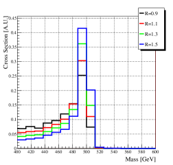
Figure 1: Reconstructed $m_{\phi}=500~{}{\rm GeV}$ from $gg\rightarrow\phi\rightarrow gg$ dijet events with FSR only (left) and with the addition of ISR/MI (right). In the absence of ISR/MI larger jet radii are preferred, while when ISR/MI are turned on a smaller radii must be used to balance the effects of contamination.

In absence of ISR/MI contamination, a large $R$ is desirable in the context of traditional jet clustering. To see why, consider the process $gg\rightarrow\phi\rightarrow gg$ where $\phi$ is a new color octet scalar with a mass of $500~{}{\rm GeV}$ and a narrow width. In a showering Monte Carlo program without hadronization, FSR is factorized from ISR/MI, so one can study the FSR in isolation. On the left side of Fig. 1, we show the distribution of the reconstructed $\phi$ mass using only FSR for various values of the anti-$k_{T}$ jet radius $R_{0}$. One sees that as $R_{0}$ increases, the reconstructed invariant mass distribution approaches the narrowly peaked distribution predicted from the hard scattering.

However, when one includes the effect of contamination, larger values of $R_{0}$ can yield poorer reconstruction, as seen from the right side of Fig. 1. Here, the jet radius that most closely matches the desired peak position is around $R_{\max}=1.1$, considerably smaller than what one would want to use considering FSR alone. From this one can see that an optimal jet algorithm would be one with a large overall jet radius that somehow avoids clustering in hadrons from ISR/MI (as well as pileup).

Figure 2: Reconstructed $m_{\phi}=500~{}{\rm GeV}$ clustered with $R_{0}=1.5$ for $gg\rightarrow\phi\rightarrow gg$ (left) and $q\bar{q}\rightarrow\phi\rightarrow q\bar{q}$ (right). The blue curve shows the reconstruction from a sample without ISR/MI. The red and black curves show data from a sample with ISR/MI, where all cells are clustered (red), and where only those cells within $\Delta R=0.2$ of an cell containing more than $1~{}{\rm GeV}$ of FSR (black). The similarity between the black and blue peaks demonstrates that considerable gains in reconstruction are possible despite the irreducible overlap in radiation.

	Improvement	$R_{0}$	$\Gamma$ [GeV]	$M$ [GeV]
	$gg\rightarrow\phi\rightarrow gg$
All cells	-	1.2	69	518
FSR cells	$309\%$	1.5	15	501
	$q\bar{q}\rightarrow\phi\rightarrow q\bar{q}$
All cells	-	0.8	31	505
FSR cells	$189\%$	1.5	11	501

Table 1: Improvement in the resonance reconstruction measure $\Delta$ presented in Sec. 4 in going from standard clustering (All cells) to an idealized situation where we only cluster those cells within $\Delta R=0.2$ of an cell containing more than $1~{}{\rm GeV}$ of FSR (FSR cells). Here $m_{\phi}=500~{}{\rm GeV}$. The definitions of $\Gamma$ and $M$ appear in Eq. (6). Because of the larger color charge of gluons compared to quarks, there is more radiation in the $gg\rightarrow\phi\rightarrow gg$ case compared to the $q\bar{q}\rightarrow\phi\rightarrow q\bar{q}$ case, so the potential improvement is correspondingly larger.

Now, there is always a minimum spatial overlap between FSR and ISR/MI from the fact that the two sources of hadrons could end up nearby in the detector. Fortunately, this overlap is relatively small. In Fig. 2 we present the $\phi$ mass reconstructed using $R_{0}=1.5$ where only those calorimeter cells within $\Delta R=0.2$  of one containing at least 1 GeV of FSR were clustered, along with the distribution obtained without this restriction. The restricted distribution is quite close to the one where only FSR was clustered, confirming the minimum spatial overlap. By considering this sort of restriction to FSR-heavy cells, one can calculate the maximum possible reconstruction improvement in going from ordinary cones to such an idealized jet algorithm. This is shown in Table 1, where the improvement is measured by the reconstruction measure $\Delta$ presented in Sec. 4. We see potential improvements of up to $3\times$ in reconstruction. Of course, such an idealized jet algorithm cannot exist since no physical observable can distinguish between FSR and ISR/MI, but the room for improvement is compelling.

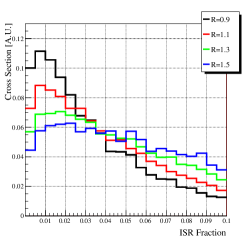
Figure 3: Fraction of a jet’s $p_{T}$ attributable to ISR/MI for $gg\rightarrow\phi\rightarrow gg$ (left) and $q\bar{q}\rightarrow\phi\rightarrow q\bar{q}$ (right).

The goal our jet trimming algorithm is to approach this ideal reconstruction as closely as possible. To do so, we need some kind of criteria to determine whether a given patch of the calorimeter is likely to contain substantial amounts of FSR. In light of the observation that ISR/MI (as well as pileup) is usually soft compared to FSR, the simplest possible criteria we have is relative transverse momentum. As shown in Fig. 3, in a typical jet ISR/MI makes up only $\mathcal{O}(1-5\%)$ of the jet’s $p_{T}$ (the contribution of pileup is a luminosity dependent question), and we saw earlier that there is minimal spatial overlap between contamination and FSR. Therefore, sources of contamination can be mitigated by simply removing patches of soft calorimeter cells.

2.2 QCD Jets vs. Boosted Objects

While the general idea of removing soft calorimeter cells is straightforward, a number of details remain unspecified. At minimum, one wants to consider patches of calorimeter cells by clustering them into subjets of radius $R_{\rm sub}>\delta_{\rm cal}=0.1$ to remove any sensitivity of the procedure to calorimeter segmentation. Beyond that, one must specify how the subjets are to be formed, how large they will be, and what will serve as the criterion for softness. As we will argue, by choosing jet trimming parameters in a way designed to enhance the reconstruction of light parton jets, we can increase reconstruction performance beyond the current techniques designed for boosted heavy particles [5, 6, 7, 8, 9, 10, 11, 12, 13, 14].

To see how one might go about choosing trimming parameters, consider first how they would be chosen to reconstruct the jet from a boosted heavy particle. Usually such a particle decays immediately into two (e.g. the Higgs or $W$/$Z$) or three (e.g. the top) final states, each at the same characteristic $p_{T}$ scale (barring a matrix element conspiracy). These states will shower into distinct hard patches in the jet (see the left panel of Fig. 4), so one can hope to remove contamination from the system by simply associating a subjet to each hard final state and discarding everything else. That is, one would discard all but the $N_{\rm cut}$ hardest subjets. Whether or not a particular subjet from a boosted heavy particle is considered soft depends upon where the subjet ranks in the subjet $p_{T}$ ordering and upon how many final state partons we expect in the decay. For instance, if we are looking to reconstruct a Higgs in its decay $h\rightarrow b\bar{b}$ we would form subjets inside the initial jet and discard all but the hardest two. In this context, the natural size of a subjet is also relatively clear; to treat each final state of the decay equally (as we should, since they have comparable $p_{T}$s) we are limited to $R_{\rm sub}\lesssim R_{0}/2$ under the assumption that the initial jet was chosen to be just large enough to encompass the entire decay of the heavy particle.

Figure 4: Comparison of a jet formed from the decay of a boosted heavy particle (left) with one from the showering of light flavor/gluons (right). Specifically, the left hand panel shows the jet formed from $h\rightarrow b\bar{b}$ while the right is a gluon jet. The ($x$, $y$)-axes are ($y$, $\phi$)-distances as measured from the jet center and the area of each calorimeter cell is proportional to its $p_{T}$.

The situation changes when we consider jets from light quarks or gluons (compare the two panels in Fig. 4). The first difference is that there is only one hard final state at lowest order in $\alpha_{s}$. Softness is therefore more naturally established directly via a cut on subjet $p_{T}$ rather than by restricting to a fixed number of subjets. Later we will establish different subjet $p_{T}$ cuts for different kinematic regimes. The second difference is that there is no natural size for the subjets as this depends upon the the $p_{T}$ cut for the subjets; a larger/smaller subjet size will necessitate a harder/softer subjet $p_{T}$ cut. With these two differences in mind, we can now define our jet trimming procedure.

3 Implementation

In this section, we present an explicit algorithm implementing the jet trimming technique outlined above. Our choice of algorithm is motivated primarily by simplicity and the ability to re-use existing jet finding procedures. Many more sophisticated choices could easily be imagined, but these are beyond the scope of the present work.

Since our jet trimming procedure will make use of well-known sequential recombination jet algorithms, we will briefly review how these work. Recall that in a recursive jet algorithm one begins with an initial set of four-momenta (these could be tracks, calorimeter cells, etc.), assigning every pair a “jet-jet distance measure” $d_{ij}$ and every individual four-momenta a “jet-beam distance measure” $d_{iB}$. The distance measures relevant for our study are:

$$\text{anti-}k_{T}~{}\cite[cite]{[\@@bibref{}{Cacciari:2008gp}{}{}]}: \qquad d_{ij}=\frac{1}{\max\left[p_{Ti}^{2},p_{Tj}^{2}\right]}\frac{R_{ij}^{2}}{R_{0}^{2}},\qquad d_{iB}=\frac{1}{p_{Ti}^{2}},$$ (1)

$$\text{C/A}~{}\cite[cite]{[\@@bibref{}{Dokshitzer:1997in,Wobisch:1998wt}{}{}]}: \qquad d_{ij}=\frac{R_{ij}^{2}}{R_{0}^{2}},\qquad d_{iB}=1,$$ (2)

$$k_{T}~{}\cite[cite]{[\@@bibref{}{Catani:1993hr,Ellis:1993tq}{}{}]}: \qquad d_{ij}=\min\left[p_{Ti}^{2},p_{Tj}^{2}\right]\frac{R_{ij}^{2}}{R_{0}^{2}},\qquad d_{iB}=p_{Ti}^{2}$$ (3)

$$\text{VR}~{}\cite[cite]{[\@@bibref{}{Krohn:2009zg}{}{}]}: \qquad d_{ij}=\frac{1}{\max\left[p_{Ti}^{2},p_{Tj}^{2}\right]}{R_{ij}^{2}},\qquad d_{iB}=\frac{\rho^{2}}{p_{Ti}^{4}}.$$ (4)

At each step in the clustering, the smallest entry in the set of all $d_{ij}$ and $d_{iB}$ is identified. When a jet-jet distance is the smallest, the corresponding four-momenta are merged, while if a jet-beam distance is the smallest, then the associated four-momentum is “merged with the beam” and set aside. Here we will deal entirely with inclusive algorithms, where the recursion continues until all jets are merged with the beam, and the algorithm returns those merged jets whose $p_{T}$ is greater than some minimum value.

3.1 Jet Trimming

The jet trimming procedure we advocate is an “outside-in” algorithm, meaning that a seed jet determined through one jet finding method is reclustered using a subjet finding method. Then a softness criteria is applied to the individual subjets to determine the final trimmed jet. One could also imagine an “inside-out” algorithm, where small subjets are found first, and clustering into a larger jet, again using some kind of softness criteria, but we will not explore that option here.

The proposed algorithm proceeds as follows:

1. Cluster all cells/tracks into jets using any clustering algorithm. The resulting jets are called the seed jets.

2. Within each seed jet, recluster the constituents using a (possibly different) jet algorithm into subjets with a characteristic radius $R_{\rm sub}$ smaller than that of the seed jet.

3. Consider each subjet, and discard the contributions of subjet $i$ to the associated seed jet if $p_{Ti}<f_{\rm cut}\cdot\Lambda_{\rm hard}$, where $f_{\rm cut}$ is a fixed dimensionless parameter, and $\Lambda_{\rm hard}$ is some hard scale chosen depending upon the kinematics of the event.

4. Assemble the remaining subjets into the trimmed jet.

This procedure is illustrated in Figs. 5 and 6. The dimensionless parameter $f_{\rm cut}$ quantifies the expected $p_{T}$ scale hierarchy between FSR and ISR/MI/pileup. In principle, this procedure could be iterated such that subjets that fail the softness criteria in one seed jet could be tested for inclusion in a different seed jet. However, this is only relevant if the original jets were effectively overlapping, or if the removal of subjets substantially changes the position of the trimmed jets relative to the original seed jets.

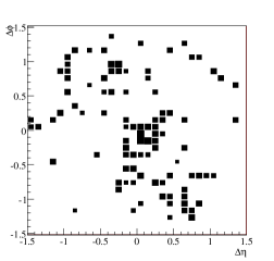
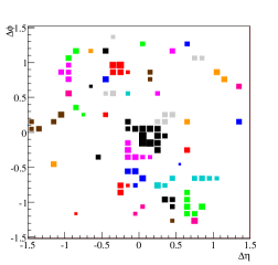
Figure 5: Step by step illustration of the jet trimming procedure. Proceeding from left to right, top to bottom, we show a jet as initially clustered (using anti-$k_{T}$ with $R_{0}=1.5$), the constituent $k_{T}$ subjets with $R_{\rm sub}=0.2$, the subjets surviving the $p_{Ti}<f_{\rm cut}\cdot p_{T}$ cut (where $f_{\rm cut}=0.03$), and the final trimmed jet. To make the figure easier to read, the area of each cell is proportional to the log of the cell’s $p_{T}$.

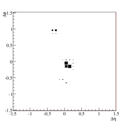
Figure 6: The jet of Fig. 5 before (top left) and after (top right) trimming using a linear scale where a cell’s area is proportional to its $p_{T}$. Also shown in the lower panel is the catchment area of the jet [4], where the empty black squares indicate cells that would have been clustered in the final trimmed jet if all cells were given an infinitesimal amount of radiation. As we will discuss more in Sec. 4.4, the jet’s area has been dramatically reduced, here to around $8\%$ of its untrimmed value.

The precise jet definition used in step 1 is largely irrelevant for the jet trimming procedure. In Sec. 4, we will trim two different jet algorithms, anti-$k_{T}$ [16] and VR [3], finding improvements in reconstruction with both.

The jet definition used in step 2, however, is more important as it determines how the subjets are found. We use the $k_{T}$ algorithm [26, 27] rather than a Cambridge-Aachen [24, 25] or anti-$k_{T}$ algorithm [16], because subjets formed by the $k_{T}$ algorithm tend to better share the energy between subjets. That is, imagine that the dominant FSR depositions in a seed jet cannot be contained within a single subjet of size $R_{\rm sub}$. In such circumstances the anti-$k_{T}$ algorithm, which clusters radiation from hardest to softest, will tend to create imbalanced subjets by allocating most of the energy to one subjet, making it more likely that the weaker subjet will be discarded when the softness criteria is applied. As the $k_{T}$ algorithm clusters from softest to hardest, it is more likely to yield a equitable distribution of energy between the subjet that contain FSR, making them less likely to be discarded by the trimming procedure.

Finally, we must select a $\Lambda_{\rm hard}$ to set our criterion of hardness when judging a subjet’s $p_{T}$. This is a non-trivial choice, as different kinematical configurations call for different scales, and the difference in reconstruction from different scale choices can be large. To illustrate this, in Sec. 4 we will present two possibilities for $\Lambda_{\rm hard}$: the seed jet’s $p_{T}$, and the effective mass of the event (i.e. the scalar sum of the transverse momenta: $H=\sum p_{T}$). While we have only considered the simplest two scale choices, it would be interesting to investigate more complicated methods to see if additional gains could be realized.

3.2 Comparison to Previous Methods

As argued before, most techniques useful in removing contamination from the jets of boosted heavy particles keep a fixed number $N_{\rm cut}$ of hard subjets. To enable an apples-to-apples comparison of $f_{\rm cut}$ vs. $N_{\rm cut}$, we will simply take the jet trimming algorithm above, replacing step 3 with:

1. Sort the subjets according to $p_{T}$ and discard the contributions of those softer than the $N_{\rm cut}$-th hardest subjet.

This allows us to employ a condensed notation in discussing various trimming procedures. We can denote different algorithms by

$${\rm alg}(\{f,N\},\{p_{T},H\}),$$ (5)

where “alg” is the algorithm used to make the seed jets (here anti-$k_{T}$ or VR), $\{f,N\}$ specifies whether we will trim all subjets with a $p_{T}$ below $f_{\rm cut}\cdot\Lambda_{\rm hard}$ or include only the $N_{\rm cut}$ hardest subjets, and the final entry (only relevant for $f_{\rm cut}$ algorithms) species whether we will use the $p_{T}$ of the seed jet or the effective mass of the event to set $\Lambda_{\rm hard}$.

In addition to this fixed $N_{\rm cut}$ algorithm—which we believe represents the most advantageous application of previous techniques for boosted objects to the study of light parton jets—we will also include a direct implementation of an algorithm from an earlier study. We will present results using the jet filtering technique of Ref. [7] (labelled Filtering below) which takes a jet and only includes those constituents that fit into the two hardest C/A subjets formed from cones of size $R_{0}/2$.

We were also interested in testing the jet pruning procedure of Ref. [11], since it could be considered as something of a middle ground between trimming and the cleaning methods that cut on a fixed number of subjets. Pruning functions by attempting to remove spurious mergings in the clustering sequence: after a seed jet is formed, its constituents are reclustered using the $k_{T}$ or C/A algorithm, and if the jet algorithm attempts to merge widely separated ($\Delta R>2R_{P}m_{J}/p_{T}$) four-momenta with a large $p_{T}$ hierarchy ($z<z_{\rm cut}$) then the merging is rejected, and the softer of the two four-momenta deleted. Pruning is most effective at removing spurious mergings from the later stages of clustering (i.e. right before the jet is complete), which is precisely what it should do to reconstruct a boosted heavy particle.

However, in our studies on pruning light quark jets we found at best only a marginal improvement in reconstruction. This occurred when the optimized value of $R_{P}$ was essentially zero, meaning that the $z_{\rm cut}$ criteria was being applied at every stage of the reconstruction. We suspect that the reason pruning is not working well in this context is that far enough down the line in the parton shower, there is no longer a clear scale separation between FSR and contamination. So while pruning employs a relative $p_{T}$ cut (as in jet trimming), it appears to be most effective when employed on a jet with a fixed, small number of hard subjets. It is an open question whether pruning techniques might be modified to successfully clean light quark jets.

4 Results

We now apply the above jet trimming procedure to two examples in different kinematic regimes: heavy resonance reconstruction, and a two-step decay chain. Our goal is justify the use of trimming, show that it is advantageous to use a trimming procedure specifically designed for jets from light partons, and to see how different measures of $\Lambda_{\rm hard}$ can change the reconstruction of the trimmed event. Unlike Sec. 2, here we will include both the effects of ISR/MI and event pileup.

In both examples, we will find that employing any sort of trimming procedure leads to an improvement in reconstruction. However, in going from an algorithm designed for boosted heavy particles to one specifically aimed at light parton jets, we can realize significant additional gains. Further, using a measure of hardness well suited to the kinematics of an event can make almost as big a difference in reconstruction as to the decision to trim in the first place.

Our results confirm our intuitions from Sec. 2 that trimming partially resolves the jet-size/contamination tradeoff. For the anti-$k_{T}$ algorithms, the optimal $R_{0}$ value in the trimmed sample is systematically larger than the optimal $R_{0}$ value in the untrimmed sample. Similar conclusions hold for VR, with the jet size parameter $\rho$ being larger in the trimmed samples. We will find that background dijet distributions are not increased through the use of a large initial radius, and may even be reduced in some cases. Finally, as expected, the active jet area [4] is substantially smaller in the trimmed sample.

To quantify reconstruction performance, we will fit reconstructed invariant mass distributions to a sum of two distributions (similar to what was done in Ref. [11]):

$$S(m)=\alpha\left[\frac{1+\beta(m-M)}{(m^{2}-M^{2})^{2}+\Gamma^{2}M^{2}}\right],$$ (6)

$$B(m)=\delta+\gamma/m,$$ (7)

where $\delta$ and $\gamma$ are restricted to be $\geq 0$. Here $S(m)$ is a skewed Breit-Wigner distribution and $B(m)$ is a background-like falling distribution. We quantify signal reconstruction via the measure

$$\Delta\equiv S(M)=\frac{\alpha}{\Gamma^{2}M^{2}},$$ (8)

i.e. the peak height of the $S(m)$ curve. While other measures of reconstruction performance would be equally reasonable, this measure favors algorithms reconstructing a tall $S(m)$ of narrow width, and has the advantage of not introducing any arbitrary parameters beyond the fitted functional form. Note that this reconstruction measure does not attempt to reward algorithms that get the right peak position, and we will see a corresponding systematic invariant mass shift in using trimmed jets.

For simplicity of discussion, we only consider processes with initial/final state gluons. From Table 1, we see that improvements are certainly possible when these are replaced with light quarks, and all of our conclusions regarding the optimal trimming method will hold there as well. It is important to remember, though, that quarks have a lower effective color charge then gluons and thus produce less QCD radiation. Thus, for light quarks one expects (and we found) a diminished optimal untrimmed jet radius and a lower potential improvement achievable through trimming.

Finally, one should keep in mind that while the improvements we find are the result of well understood physical effects, the precise values of the trimming parameters will change somewhat when the Monte Carlo tuning is adjusted to account for LHC data. Thus, while the parameters below will provide a reasonable guide to what should be used at the LHC, the exact values will need to be inferred from a iterative process of Monte Carlo tuning to standard candles.

4.1 Heavy Resonance Decays

The simplest test of a jet algorithm is how it reconstructs a heavy resonance decaying to the two jets. As in Sec. 2, we use the process $gg\rightarrow\phi\rightarrow gg$ where $\phi$ is a color octet scalar with $m_{\phi}=500~{}{\rm GeV}$.

	Improvement	$f_{\rm cut}$, $N_{\rm cut}$	$R_{\rm sub}$	$R_{0}$, $\rho$	$\Gamma$ [GeV]	$M$ [GeV]
anti-$k_{T}$	-	-	-	$1.0^{\ast}$	$71$	$522$
anti-$k_{T}$ ($N$)	$40\%$	$5^{\ast}$	$0.2^{\ast}$	$1.5^{\ast}$	$62$	$499$
anti-$k_{T}$ ($f$, $p_{T}$)	$59\%$	$3\times 10^{-2\ast}$	0.2	1.5	$52$	$475$
anti-$k_{T}$ ($f$, $H$)	$61\%$	$1\times 10^{-2\ast}$	0.2	1.5	$50$	$478$
VR	$30\%$	-	-	$200^{\ast}~{}{\rm GeV}$	$62$	$511$
VR ($N$)	$53\%$	$5$	0.2	$275^{\ast}~{}{\rm GeV}$	$53$	$498$
VR ($f$, $p_{T}$)	$68\%$	$3\times 10^{-2}$	$0.2$	$300^{\ast}~{}{\rm GeV}$	$49$	$475$
VR ($f$, $H$)	$73\%$	$1\times 10^{-2}$	$0.2$	$300^{\ast}~{}{\rm GeV}$	$47$	$478$
Filtering	$27\%$	2	$R_{0}/2$	$1.3^{\ast}$	$61$	$515$

Table 2: Comparison of dijet resonance reconstruction using trimmed and untrimmed algorithms. The first column specifies the algorithm, the second lists the change in $\Delta$ over untrimmed anti-$k_{T}$ (second row), the third lists the relevant trimming parameters, the fourth contains the subjet radius, the fifth the seed jet parameters, the sixth the fitted width, and the seventh the fitted mass. For each algorithm, we have optimized those parameters denoted by a ^∗, while the rest have remained fixed.

The results of this reconstruction are presented in Table 2. Here we are interested primarily in two different comparisons: untrimmed algorithms versus those trimmed using an $f_{\rm cut}$ (so as to measure the full potential for improvement in reconstruction), and those trimmed using an $N_{\rm cut}$ to those using an $f_{\rm cut}$. Now, the more parameter choices one optimizes in an algorithm the more that algorithm stands to gain from arbitrary statistical fluctuations. To guard against this and ensure that the first comparison above is fair, we fully optimize the anti-$k_{T}$ ($N$) algorithm, using the resulting best choices of $R_{\rm sub}$ and $R_{0}$ as inputs to our optimization of anti-$k_{T}$ ($f$), for which we only optimize a single parameter: $f_{\rm cut}$. The result is a fair comparison of untrimmed algorithms to those trimmed with an $f_{\rm cut}$, and a comparison of $N_{\rm cut}$ to $f_{\rm cut}$ trimming where $N_{\rm cut}$ trimming is given a statistical advantage.

Several algorithms and trimming procedures are presented in Table 2. We have included untrimmed anti-$k_{T}$, anti-$k_{T}$ with a cut on the momenta of $k_{T}$ subjets (set relative to both the jet’s $p_{T}$ and the event’s effective mass), anti-$k_{T}$ with a fixed number of $k_{T}$ subjets, and for comparison with previous techniques anti-$k_{T}$ with two C/A subjets of half the seed jet radius (i.e. the filtering procedure of Ref. [7]). Both trimmed and untrimmed VR jets are also included. In Fig. 7, we display the reconstructed $\phi$ mass using both trimmed and untrimmed anti-$k_{T}$ and VR algorithms.

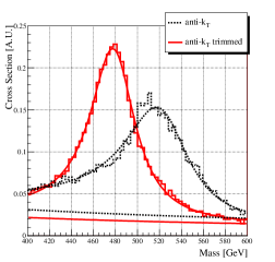
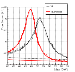
Figure 7: Dijet resonance reconstruction with and without trimming using the anti-$k_{T}$/VR and anti-$k_{T}$/VR ($f$, $H$) algorithms. The algorithm parameters are those that optimize the $\Delta$ measure of Eq. (8), as listed in Table 2. The upper curves are fitted to the sum of $S(m)$ and $B(m)$ from Eqs. (6) and (7), while the lower curves display the contribution of $B(m)$.

We see that trimming of any sort is useful in reconstruction. However, the difference between trimming techniques is apparent. By using an algorithm with a $p_{T}$ cut determined as a fraction of the original $p_{T}$ (i.e. the samples whose trimming is parameterized by an $f_{\rm cut}$) we are able to see significant gains beyond what is possible using a fixed number of subjets. This reflects the fact that the structure of the jet from a light parton is not known a-priori, unlike the jets from boosted heavy particles, so it is advantageous to trim with a direct subjet $p_{T}$ cut. We further note that at this stage, the difference between using $H$ and $p_{T}$ to set $\Lambda_{\rm hard}$ makes only a small difference in reconstruction, reflecting the fact that for dijet events $p_{T}\approx H/2$. Below, we will see that the situation will change in more complicated event topologies.

Before continuing, we remark that in Fig. 7, the dijet invariant mass distribution is systematically shifted to lower values through the effects of jet trimming. This is to be expected, given that the trimming procedure will necessarily result in some accidental removal of FSR. To understand the size of the effect, note that in Table 2 we find an optimized $f_{\rm cut}$ of around $3\%$ when we cut on the subjet’s $p_{T}$ relative to that of the seed jet, and that the optimal $N_{\rm cut}$ for fixed-number cleaning is 5. Since the pattern of QCD radiation from a light parton ensures us that the subjets follow a strong $p_{T}$ hierarchy, we should only expect one or two subjets to be slightly below the $3\%$ $p_{T}$ cut we have imposed. This is enough to account for the roughly $5\%$ shift in $M$ that we observe.

4.2 Longer Decay Chains

Next, we consider the production channel $gg\rightarrow X\rightarrow YY\rightarrow gggg$ where $m_{X}=1~{}{\rm TeV}$ and $m_{Y}=300~{}{\rm GeV}$. This sample is qualitatively different from the dijet reconstruction in two ways: the final state is more crowded, and the final state jets can vary widely in $p_{T}$ within the same event. The results from this reconstruction are presented in Table 3, and the resulting $m_{X}$ and $m_{Y}$ distributions are plotted in Fig. 8 and Fig. 9, respectively.

	Improvement	$f_{\rm cut}$, $N_{\rm cut}$	$R_{\rm sub}$	$R_{0}$, $\rho$	$\Gamma$ [GeV]	$M$ [GeV]
anti-$k_{T}$	-	-	-	$0.8^{\ast}$	$158$	$994$
anti-$k_{T}$ ($N$)	$12\%$	$5^{\ast}$	$0.2^{\ast}$	$1.0^{\ast}$	$115$	$969$
anti-$k_{T}$ ($f$, $p_{T}$)	$10\%$	$3\times 10^{-2\ast}$	0.2	1.0	$108$	$941$
anti-$k_{T}$ ($f$, $H$)	$19\%$	$5\times 10^{-3\ast}$	0.2	1.0	$100$	$944$
VR	$10\%$	-	-	$150^{\ast}~{}{\rm GeV}$	$157$	$979$
VR ($N$)	$17\%$	$5$	$0.2$	$275^{\ast}~{}{\rm GeV}$	$115$	$965$
VR ($f$, $p_{T}$)	$16\%$	$3\times 10^{-2}$	$0.2$	$225^{\ast}~{}{\rm GeV}$	$112$	$938$
VR ($f$, $H$)	$22\%$	$5\times 10^{-3}$	$0.2$	$300^{\ast}~{}{\rm GeV}$	$101$	$942$
Filtering	$6\%$	2	$R_{0}/2$	$0.9^{\ast}$	$128$	$969$

Table 3: Comparison of the $2\rightarrow 4$ resonance reconstruction using trimmed and untrimmed algorithms. Reconstruction is performed by taking the invariant mass of the hardest four jets. The first column specifies the algorithm, the second lists the change in $\Delta$ over untrimmed anti-$k_{T}$ (second row), the third lists the trimming parameters, the fourth contains the subjet radius, the fifth the seed jet parameters, the sixth the fitted width, and the seventh the fitted mass. For each algorithm we have optimized those parameters denoted by a ^∗, while the rest have remained fixed.

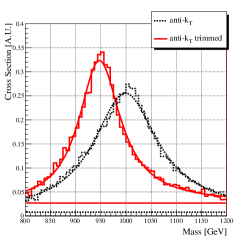
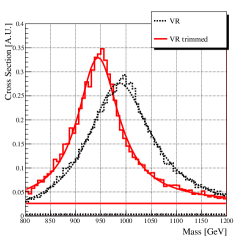
Figure 8: Reconstruction of the resonance $m_{X}=1~{}{\rm TeV}$ in $gg\rightarrow X\rightarrow YY\rightarrow gggg$ with and without trimming using the anti-$k_{T}$/VR and anti-$k_{T}$/VR ($f$, $H$) algorithms. The algorithm parameters are those optimized to those that optimize the $\Delta$ measure of Eq. (8), as listed in Table 3. The upper curves are fitted to the sum of $S(m)$ and $B(m)$ from Eqns. (6) and (7), while the lower curves represent the contribution of $B(m)$.

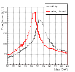
Figure 9: Reconstruction of the intermediate resonance mass $m_{Y}=300~{}{\rm GeV}$ in the process $gg\rightarrow X\rightarrow YY\rightarrow gggg$ using the anti-$k_{T}$/VR and anti-$k_{T}$/VR ($f$,$H$) parameters of Table 3. These distributions are formed by taking the four hardest jets in each event, considering the two masses from every possible $2\times 2$ partition of these jets, and plotting the masses from the most equitable partition (defined as the one for which $m_{\rm min}/m_{\rm max}$ is closest to one).

That the final state is crowded somewhat limits the improvements achievable from trimming. We saw before in Table 2 that trimming seemed to work well when the seed jets were allowed to grow much larger than the optimized untrimmed jets. Here, the untrimmed jets are optimized at $R_{0}=0.8$, so the trimmed jets cannot grow much larger without merging with each other and ruining the reconstruction. Despite this limitation, however, we see that valuable improvements are still possible.

More importantly, now we see that the choice of $\Lambda_{\rm hard}$ can make a significant difference in reconstruction. When $\Lambda_{\rm hard}$ is chosen to be the effective mass of the event, reconstruction is improved beyond the case where $\Lambda_{\rm hard}$ is the seed jet $p_{T}$ (the improvement roughly doubles). This is because when we let the seed jet $p_{T}$ determine the hard scale for each jet while using a fixed $f_{\rm cut}$, the softer jets will see little trimming (because the minimum subjet $p_{T}$ is soft), while for the same reason the harder jets will see too much trimming. The resolution, it seems, is to simply use a global $p_{T}$ cutoff for each event when the signal jets are of different characteristic $p_{T}$ scales.

4.3 Dijet Backgrounds

The improvements in signal reconstruction seen so far would be of little use if jet trimming significantly increased the background as well. After all, to see improvements in signal reconstruction we must let our seed jets cluster with a large radius, and it is possible that this could result in an unintended rise in the background distributions.

Figure 10: Standard model QCD dijet background reconstruction with and without trimming using the anti-$k_{T}$/VR and anti-$k_{T}$/VR ($f$, $H$) algorithms and the optimized signal parameters from Table 2.

Fortunately, this does not seem to be the case. In Fig. 10 we present the background QCD dijet invariant mass distributions clustered using the parameters of Table 2 optimized for signal reconstruction. If anything, we see that the trimmed distributions are shifted to lower invariant mass values than the untrimmed distributions. This is especially useful in the case of the VR jet algorithm, which on its own can distort background distributions to higher values. It is tempting to argue from this that trimming can also be useful in reducing the background, but one should be careful drawing such a conclusion as the signal position also shifts. The precise signal and background interplay, while intriguing, is therefore likely to be highly process dependent, and requires a dedicated study.

4.4 Jet Area

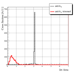
Figure 11: Jet area, defined as the area of calorimeter cells clustered into a jet if each cell contains at least an infinitesimal about of radiation, for anti-$k_{T}$ vs. anti-$k_{T}$($f$, $H$) (left panel) and VR vs. VR($f$, $H$) (right panel), using the optimized parameters from Table 2. The area of the untrimmed algorithm is roughly $\pi R_{0}^{2}$, as expected, while the trimmed jet’s area is much smaller.

In Fig. 2, we argued that the overlap of ISR/MI with FSR was minimal, so even though the naive area of the jets employed in our analysis is quite large, there should not be significant sensitivity to the effects of ISR/MI/pileup that we set out to avoid. We can quantify this statement using the catchment area of a jet [4], allowing us to directly measure the sensitivity of the trimmed jet to uniform diffuse contamination. We find that while the jets we use in trimming start with large areas, after the jet trimming procedure is applied the active area decreases dramatically, as shown in Fig. 11. In fact, the active area after trimming is even less than that of the untrimmed jet which began with a smaller radius.

One caution, however, is that the catchment area only captures the sensitivity to soft contamination. Trimming cannot guard against a fluctuation of ISR/MI/pileup that yields a hard subjet above the $f_{\rm cut}$ threshold. In some ways, trimming accentuates such fluctuations, since the contamination cannot be averaged over a larger jet area and subtracted statistically using, e.g. the methods of Ref. [4]. Therefore, more detailed studies are needed to really understand such systematic biases.

5 Conclusions

In this paper, we have proposed jet trimming as a way to improve jet reconstruction by mitigating the spatial overlap between FSR and ISR/MI/pileup in hadronic collisions. This technique actively removes sources of contamination by exploiting the difference in scale between the hard emissions of FSR and the relatively soft emissions from ISR/MI/pileup. While prior efforts had been made along similar lines, those efforts focused on removing contamination from the jets of heavy boosted objects. We have shown that light parton jets benefit from methods that emphasize relative subjet $p_{T}$ instead of the number of subjets.

We presented an explicit algorithm that implements jet trimming. Our algorithm begins with seed jets constructed through any means (here we employ anti-$k_{T}$ and VR), which are then reclustered using an inclusive $k_{T}$ algorithm and trimmed according to a subjet $p_{T}$ cut set relative to some hard scale determined by the kinematics of the event. In two different kinematic configurations, we find large improvements in reconstruction efficiency from using trimmed jets. Moreover, unlike our previous VR algorithm [3], this improvement was obtained without a drastic increase in the catchment area of the jet.

Further study is necessary to understand how this jet trimming procedure would affect jet systematic errors in an actual experimental context. For example, jet energy scale systematics already require a correction from ISR/MI/pileup contamination, and exactly how a jet energy correction would be applied in the case of trimmed jets is unclear. However, by addressing ISR/MI/pileup contamination on a jet-by-jet basis, we expect that the systematic uncertainty associated with trimmed jets should not be any worse than for fixed-radius jets. Moreover, it would be interesting to see whether the systematic shift in the invariant mass peak from accidentally throwing away FSR subjets could be fixed through a simple jet energy rescaling.

Finally, while the improvement in reconstruction from trimming is already quite helpful, it is nowhere near the in-principle improvement we saw in Sec. 2. Perhaps further advances can be made through a better choice of the $\Lambda_{\rm hard}$ parameter or a different subjet finding procedure. Whether any jet trimming algorithm can ever hope to approach the theoretical limit in ISR/MI/pileup rejection is an important open question, but the gains already seen in a simple trimming algorithm recommend its use at the LHC.

- [1] S. D. Ellis, J. Huston, K. Hatakeyama, P. Loch, and M. Tonnesmann, Jets in hadron-hadron collisions, Prog. Part. Nucl. Phys. 60 (2008) 484–551, [0712.2447].
- [2] G. P. Salam, Towards Jetography, 0906.1833.
- [3] D. Krohn, J. Thaler, and L.-T. Wang, Jets with Variable R, JHEP 06 (2009) 059, [0903.0392].
- [4] M. Cacciari, G. P. Salam, and G. Soyez, The Catchment Area of Jets, JHEP 04 (2008) 005, [0802.1188].
- [5] M. H. Seymour, Searches for new particles using cone and cluster jet algorithms: A Comparative study, Z. Phys. C62 (1994) 127–138.
- [6] J. M. Butterworth, B. E. Cox, and J. R. Forshaw, scattering at the CERN LHC, Phys. Rev. D65 (2002) 096014, [hep-ph/0201098].
- [7] J. M. Butterworth, A. R. Davison, M. Rubin, and G. P. Salam, Jet substructure as a new Higgs search channel at the LHC, Phys. Rev. Lett. 100 (2008) 242001, [0802.2470].
- [8] T. Plehn, G. P. Salam, and M. Spannowsky, Fat Jets for a Light Higgs, 0910.5472.
- [9] G. Brooijmans, High hadronic top quark identification, Tech. Rep. ATL-COM-PHYS-2008-001, ATLAS, Feb, 2008.
- [10] D. E. Kaplan, K. Rehermann, M. D. Schwartz, and B. Tweedie, Top Tagging: A Method for Identifying Boosted Hadronically Decaying Top Quarks, Phys. Rev. Lett. 101 (2008) 142001, [0806.0848].
- [11] S. D. Ellis, C. K. Vermilion, and J. R. Walsh, Techniques for improved heavy particle searches with jet substructure, Phys. Rev. D80 (2009) 051501, [0903.5081].
- [12] S. D. Ellis, C. K. Vermilion, and J. R. Walsh, Recombination Algorithms and Jet Substructure: Pruning as a Tool for Heavy Particle Searches, 0912.0033.
- [13] J. M. Butterworth, J. R. Ellis, and A. R. Raklev, Reconstructing sparticle mass spectra using hadronic decays, JHEP 05 (2007) 033, [hep-ph/0702150].
- [14] J. M. Butterworth, J. R. Ellis, A. R. Raklev, and G. P. Salam, Discovering baryon-number violating neutralino decays at the LHC, 0906.0728.
- [15] M. Cacciari, J. Rojo, G. P. Salam, and G. Soyez, Quantifying the performance of jet definitions for kinematic reconstruction at the LHC, JHEP 12 (2008) 032, [0810.1304].
- [16] M. Cacciari, G. P. Salam, and G. Soyez, The anti- jet clustering algorithm, JHEP 04 (2008) 063, [0802.1189].
- [17] T. Sjostrand, S. Mrenna, and P. Skands, PYTHIA 6.4 Physics and Manual, JHEP 05 (2006) 026, [hep-ph/0603175].
- [18] CDF Collaboration, R. D. Field, The underlying event in hard scattering processes, hep-ph/0201192.
- [19] CDF Collaboration, R. Field and R. C. Group, PYTHIA tune A, HERWIG, and JIMMY in Run 2 at CDF, hep-ph/0510198.
- [20] M. Cacciari, G. Salam, and G. Soyez, “FastJet.” http://fastjet.fr/.
- [21] M. Cacciari and G. P. Salam, Dispelling the myth for the jet-finder, Phys. Lett. B641 (2006) 57–61, [hep-ph/0512210].
- [22] B. Andersson, The Lund model, Camb. Monogr. Part. Phys. Nucl. Phys. Cosmol. 7 (1997) 1–471.
- [23] ALEPH Collaboration, R. Barate et al., Studies of quantum chromodynamics with the ALEPH detector, Phys. Rept. 294 (1998) 1–165.
- [24] Y. L. Dokshitzer, G. D. Leder, S. Moretti, and B. R. Webber, Better Jet Clustering Algorithms, JHEP 08 (1997) 001, [hep-ph/9707323].
- [25] M. Wobisch and T. Wengler, Hadronization corrections to jet cross sections in deep- inelastic scattering, hep-ph/9907280.
- [26] S. Catani, Y. L. Dokshitzer, M. H. Seymour, and B. R. Webber, Longitudinally invariant K(t) clustering algorithms for hadron hadron collisions, Nucl. Phys. B406 (1993) 187–224.
- [27] S. D. Ellis and D. E. Soper, Successive combination jet algorithm for hadron collisions, Phys. Rev. D48 (1993) 3160–3166, [hep-ph/9305266].
- [28] C. K. Vermilion, “FastPrune.” http://bit.ly/pruning.