The exclusive Bβ†’Kβˆ—(β†’KΟ€)l+lβˆ’B\to K^{*}(\to K\pi)l^{+}l^{-} decay:
CP conserving observables.††thanks: Presented by J. Matias at Flavianet Meeting, Kazimierz, July 2009,
CERN-PH-TH/2009-207, MZ-TH/09-44, IC/HEP/09-14, UAB-FT-673

U. Egede1    T. Hurth2,3    J. Matias4    M. Ramon4    W. Reece1 1 Imperial College London, London SW7Β 2AZ, United Kingdom
2 CERN, Dept. of Physics, Theory Division, CH-1211 Geneva 23, Switzerland
3 Institute for Physics, Johannes Gutenberg-University, D-55099 Mainz, Germany
4 IFAE, Universitat AutΓ²noma de Barcelona, 08193 Bellaterra, Barcelona, Spain
Abstract

We study the K* polarization states in the exclusive 4-body B meson decay B0β†’Kβˆ—0(β†’Kβˆ’Ο€+)l+lβˆ’B^{0}\to K^{*0}(\to K^{-}\pi^{+})l^{+}l^{-} in the low dilepton mass region working in the framework of QCDF. We review the construction of the CP conserving transverse and transverse/longitudinal observables AT2superscriptsubscript𝐴𝑇2A_{T}^{2}, AT3superscriptsubscript𝐴𝑇3A_{T}^{3} and AT4superscriptsubscript𝐴𝑇4A_{T}^{4}. We focus here, on analyzing their behaviour at large recoil energy in presence of right-handed currents.

\PACS

13.25.Hw,11.30.Hv,12.39.St

1 Motivation

The exclusive decay Bβ†’Kβˆ—β€‹l+​lβˆ’β†’π΅superscript𝐾superscript𝑙superscript𝑙B\to K^{*}l^{+}l^{-} will play a central role in the near future at LHCb and also at Super-LHCb. This channel is particularly interesting because it provides information in different ways. It is used as a basis to construct different type of observables, such as the forward-backward (FB) asymmetry [1, 2], the isospin asymmetry [3] and the angular distribution observables [4, 5, 6, 7, 8, 9]. Here, we will focus on the observables derived from the 4-body decay distribution: Bβ†’Kβˆ—(β†’KΟ€)l+lβˆ’B\to K^{*}(\to K\pi)l^{+}l^{-} that provides information on the K* spin amplitudes.

2 Differential decay distributions, K* Spin Amplitudes and Non Minimal Supersymmetric model

The starting point is the differential decay distribution of the decay πΒ―πβ†’πŠΒ―βˆ—πŸŽ(β†’πŠΟ€)π₯+π₯βˆ’{\bf{\bar{B}_{d}}\to{\bar{K}^{*0}}(\to K\pi)l^{+}l^{-}}. This distribution with the Kβˆ—0superscript𝐾absent0K^{*0} on the mass shell is described by s𝑠{s} and three angles ΞΈπ₯subscriptπœƒπ₯{\bf\theta_{l}} (angle between ΞΌβˆ’superscriptπœ‡\mu^{-} and the direction of the outgoing Kβˆ—superscript𝐾K^{*} in ΞΌβ€‹ΞΌπœ‡πœ‡\mu\mu frame) , θ𝐊subscriptπœƒπŠ{\bf\theta_{K}} (angle between Kβˆ’superscript𝐾K^{-} and outgoing Kβˆ—superscript𝐾K^{*} in KΒ―βˆ—superscript¯𝐾\bar{K}^{*} frame) and Ο•italic-Ο•{\bf\phi} (angle between the two planes),

d4​Γd​q2​d​θl​d​θK​d​ϕ=932​π​I​(q2,ΞΈl,ΞΈK,Ο•)​sin⁑θl​sin⁑θKsuperscript𝑑4Γ𝑑superscriptπ‘ž2𝑑subscriptπœƒπ‘™π‘‘subscriptπœƒπΎπ‘‘italic-Ο•932πœ‹πΌsuperscriptπ‘ž2subscriptπœƒπ‘™subscriptπœƒπΎitalic-Ο•subscriptπœƒπ‘™subscriptπœƒπΎ\frac{d^{4}\Gamma}{d{q^{2}}\,d{\theta_{l}}\,d{\theta_{K}}\,d{\phi}}=\frac{9}{32\pi}I({q^{2}},{\theta_{l},{\theta_{K}},{\phi}})\sin{\theta_{l}}\sin{\theta_{K}}\>

where I=𝐈𝟏+𝐈𝟐cos2ΞΈl+πˆπŸ‘sin2ΞΈlcos2Ο•+πˆπŸ’sin2ΞΈlcosΟ•+πˆπŸ“sinΞΈlcosΟ•++πˆπŸ”cosΞΈl+πˆπŸ•sinΞΈlsinΟ•+πˆπŸ–sin2ΞΈlsinΟ•+πˆπŸ—sin2ΞΈlsin2Ο•.I={\bf I_{1}}+{\bf I_{2}}\cos 2\theta_{l}+{\bf I_{3}}\sin^{2}\theta_{l}\cos 2\phi+{\bf I_{4}}\sin 2\theta_{l}\cos\phi+{\bf I_{5}}\sin\theta_{l}\cos\phi++{\bf I_{6}}\cos\theta_{l}+{\bf I_{7}}\sin\theta_{l}\sin\phi+{\bf I_{8}}\sin 2\theta_{l}\sin\phi+{\bf I_{9}}\sin^{2}\theta_{l}\sin 2\phi. In the massless limit the I’s are function of the K* spin amplitudes[4] AβŸ‚L,Rsubscript𝐴perpendicular-toabsent𝐿𝑅A_{\perp L,R}, Aβˆ₯L,RA_{\|L,R} and A0​L,Rsubscript𝐴0𝐿𝑅A_{0L,R}, we have then 6 complex amplitudes, four symmetries (see [7]) and 9 IisubscriptIi\rm I_{i} parameters, of which 8 are independent. At this point we can follow two alternatives to construct observables: a) fit the parameters I’s, use them as observables, and compare the predictions with data or b) use the spin amplitudes as the key ingredient to construct a selected group of observables.

The first option (β€˜a’)[8] is experimentally problematic as the resultant fit fails to capture the correlation between the I’s induced by the underlying K* spin amplitudes. The second option (β€˜b’)[6] aims at constructing selected observables from the K* spin amplitudes that are extracted directly from the experimental fit. Certain criteria are considered: maximal sensitivity to right-handed currents (RH), minimal sensitivity to poorly known soft form factors, and good experimental resolution. We will always follow option β€˜b’[6]. The procedure in this case is the following: choose the combination of spin amplitudes with maximal sensitivity to RH currents; check if the combination fulfills all symmetries; and finally, analyse the observables and New Physics (NP) impact. Notice that these combinations of spin amplitudes may be simple functions of the I’s (see [6]) or highly non-linear combinations showing up an interesting sensitivity to NP (see [7] for an example).

The keypoint is the evaluation of the relevant matrix elements that in naive factorization are functions of the form factors V​(q2)𝑉superscriptπ‘ž2V(q^{2}), A0,1,2,3​(q2)subscript𝐴0123superscriptπ‘ž2A_{0,1,2,3}(q^{2}) and T1,2,3​(q2)subscript𝑇123superscriptπ‘ž2T_{1,2,3}(q^{2}). Then the spin amplitudes AβŸ‚,βˆ₯,0A_{\perp,\|,0} can be written in terms of these form factors and the Wilson coefficients C7effsuperscriptsubscript𝐢7effC_{7}^{\mathrm{eff}}, C7eff⁣′superscriptsubscript𝐢7effβ€²C_{7}^{\mathrm{eff}\prime}, C9effsuperscriptsubscript𝐢9effC_{9}^{\mathrm{eff}} and C10subscript𝐢10C_{10} of an effective Hamiltonian that includes RH currents via the electromagnetic dipole operator O7β€²=(e/16​π2)​mb​(s¯​σμ​ν​PL​b)​Fμ​νsuperscriptsubscript𝑂7′𝑒16superscriptπœ‹2subscriptπ‘šπ‘Β―π‘ subscriptπœŽπœ‡πœˆsubscript𝑃𝐿𝑏superscriptπΉπœ‡πœˆO_{7}^{\prime}=(e/16\pi^{2})m_{b}(\bar{s}\sigma_{\mu\nu}P_{L}b)F^{\mu\nu}:

𝐀βŠ₯𝐋,𝐑=N^​λ1/2​[(C9effβˆ“C10)​V​(q2)mB+mKβˆ—+2​mbq2​(C7eff+C7eff⁣′)​T1​(q2)]subscript𝐀bottom𝐋𝐑^𝑁superscriptπœ†12delimited-[]minus-or-plussubscriptsuperscript𝐢eff9subscript𝐢10𝑉superscriptπ‘ž2subscriptπ‘šπ΅superscriptsubscriptπ‘šπΎ2subscriptπ‘šπ‘superscriptπ‘ž2subscriptsuperscript𝐢eff7subscriptsuperscript𝐢effβ€²7subscript𝑇1superscriptπ‘ž2{\bf A_{\bot L,R}}={\hat{N}}\lambda^{1/2}\bigg{[}({C^{\rm eff}_{9}}\mp{C_{10}})\frac{V(q^{2})}{m_{B}+m_{K}^{*}}+\frac{2m_{b}}{q^{2}}({C^{\rm eff}_{7}}+{C^{\rm eff\prime}_{7}}){T_{1}(q^{2})}\bigg{]}
𝐀βˆ₯𝐋,𝐑=βˆ’N^​(mB2βˆ’mKβˆ—2)​[(C9effβˆ“C10)​A1​(q2)mBβˆ’mKβˆ—+2​mbq2​(C7effβˆ’C7eff⁣′)​T2​(q2)]{\bf A_{\|L,R}}\!=\!-{\hat{N}}(m_{B}^{2}-m_{K^{*}}^{2})\bigg{[}({C^{\rm eff}_{9}}\mp{C_{10}})\frac{A_{1}(q^{2})}{m_{B}-m_{K^{*}}}+\frac{2m_{b}}{q^{2}}({C^{\rm eff}_{7}}-{C^{\rm eff\prime}_{7}}){T_{2}(q^{2})}\bigg{]}
π€πŸŽβ€‹π‹,𝐑subscript𝐀0𝐋𝐑\displaystyle{\bf A_{0L,R}} =\displaystyle\!\!=\!\! βˆ’N^2​mKβˆ—β€‹2​q2[(C9effβˆ“C10){(mB2βˆ’mKβˆ—2βˆ’q2)(mB+mKβˆ—)A1(q2)\displaystyle-\frac{\hat{N}}{2m_{K^{*}}\sqrt{2q^{2}}}\bigg{[}({C^{\rm eff}_{9}}\mp{C_{10}})\bigg{\{}(m_{B}^{2}-m_{K^{*}}^{2}-q^{2})(m_{B}+m_{K^{*}}){A_{1}(q^{2})}
βˆ’Ξ»A2​(q2)mB+mKβˆ—}+2mb(C7effβˆ’C7eff⁣′){(mB2+3mKβˆ—2βˆ’q2)T2(q2)\displaystyle-\lambda\frac{A_{2}(q^{2})}{m_{B}+m_{K^{*}}}\bigg{\}}+{2m_{b}}({C^{\rm eff}_{7}}-{C^{\rm eff\prime}_{7}})\bigg{\{}(m_{B}^{2}+3m_{K^{*}}^{2}-q^{2}){T_{2}(q^{2})}
βˆ’Ξ»mB2βˆ’mKβˆ—2T3(q2)}],\displaystyle-\frac{\lambda}{m_{B}^{2}-m_{K^{*}}^{2}}{T_{3}(q^{2})}\bigg{\}}\bigg{]},

We are left again with two possible choices: either i) use QCD light cone sum rules (LCSR) to estimate the required form factors adding the Ξ±ssubscript𝛼𝑠\alpha_{s} corrections from QCDF or ii) work consistently in the same framework of QCDF at LO and NLO [2] and include a reasonable conservative size for the possible Ξ›/mbΞ›subscriptπ‘šπ‘\Lambda/m_{b} corrections. The first option (β€˜i’)[8] implies neglecting some π’ͺ​(Ξ›/mb)π’ͺΞ›subscriptπ‘šπ‘{\cal O}(\Lambda/m_{b}) corrections to QCDF and assume that the main part of those corrections are inside the soft form factors evaluated with QCD LCSR. The second option (β€˜ii’)[6] allows us to explore the impact that π’ͺ​(Ξ›/mb)π’ͺΞ›subscriptπ‘šπ‘{\cal O}(\Lambda/m_{b}) corrections have on the observables.

In the limit mBβ†’βˆžβ†’subscriptπ‘šπ΅m_{B}\to\infty and EKβˆ—β†’βˆžβ†’superscriptsubscript𝐸𝐾E_{K}^{*}\to\infty all form factors are related to only two soft form factors ΞΎβŸ‚subscriptπœ‰perpendicular-to\xi_{\perp} and ΞΎβˆ₯subscriptπœ‰βˆ₯\xi_{\|} [10] and consequently transversity amplitudes simplify enormously; then observables can be easily constructed in which the soft form factors cancel out completely at LO:

𝐀βŠ₯𝐋,𝐑=N^​mB​(1βˆ’s^)​[(C9effβˆ“C10)+2​m^bs^​(C7eff+C7eff⁣′)]​ξβŠ₯​(EKβˆ—),subscript𝐀bottom𝐋𝐑^𝑁subscriptπ‘šπ΅1^𝑠delimited-[]minus-or-plussubscriptsuperscript𝐢eff9subscript𝐢102subscript^π‘šπ‘^𝑠subscriptsuperscript𝐢eff7subscriptsuperscript𝐢effβ€²7subscriptπœ‰bottomsubscript𝐸superscript𝐾{\bf A_{\bot L,R}}={\hat{N}}m_{B}(1-\hat{s})\bigg{[}({C^{\rm eff}_{9}}\mp{C_{10}})+\frac{2\hat{m}_{b}}{\hat{s}}({C^{\rm eff}_{7}}+{C^{\rm eff\prime}_{7}})\bigg{]}\xi_{\bot}(E_{K^{*}}),
𝐀βˆ₯𝐋,𝐑=βˆ’N^​mB​(1βˆ’s^)​[(C9effβˆ“C10)+2​m^bs^​(C7effβˆ’C7eff⁣′)]​ξβŠ₯​(EKβˆ—),{\bf A_{\|L,R}}=-{\hat{N}}m_{B}(1-\hat{s})\bigg{[}({C^{\rm eff}_{9}}\mp{C_{10}})+\frac{2\hat{m}_{b}}{\hat{s}}({C^{\rm eff}_{7}}-{C^{\rm eff\prime}_{7}})\bigg{]}\xi_{\bot}(E_{K^{*}}),
π€πŸŽβ€‹π‹,𝐑=βˆ’N^​mB2​m^Kβˆ—β€‹2​s^​(1βˆ’s^)2​[(C9effβˆ“C10)+2​m^b​(C7effβˆ’C7eff⁣′)]​ξβˆ₯​(EKβˆ—),subscript𝐀0𝐋𝐑^𝑁subscriptπ‘šπ΅2subscript^π‘šsuperscript𝐾2^𝑠superscript1^𝑠2delimited-[]minus-or-plussubscriptsuperscript𝐢eff9subscript𝐢102subscript^π‘šπ‘subscriptsuperscript𝐢eff7subscriptsuperscript𝐢effβ€²7subscriptπœ‰βˆ₯subscript𝐸superscript𝐾\displaystyle{\bf A_{0L,R}}=-\frac{{\hat{N}}m_{B}}{2\hat{m}_{K^{*}}\sqrt{2\hat{s}}}(1-\hat{s})^{2}\bigg{[}({C^{\rm eff}_{9}}\mp{C_{10}})+2\hat{m}_{b}({C^{\rm eff}_{7}}-{C^{\rm eff\prime}_{7}})\bigg{]}\xi_{\|}(E_{K^{*}}),

where s^=q2/mB2^𝑠superscriptπ‘ž2superscriptsubscriptπ‘šπ΅2\hat{s}=q^{2}/m_{B}^{2}, m^b=mb/mBsubscript^π‘šπ‘subscriptπ‘šπ‘subscriptπ‘šπ΅\hat{m}_{b}=m_{b}/m_{B} and m^Kβˆ—=mKβˆ—/mBsubscript^π‘šsuperscript𝐾subscriptπ‘šsuperscript𝐾subscriptπ‘šπ΅\hat{m}_{K^{*}}=m_{K^{*}}/m_{B}.

Finally, our BSM testing ground model will be a Supersymmetric model with non-minimal flavour violation in the down squark sector that induces RH currents[5]. We will focus on two scenarios[6]:

  • β€’

    Scenario A: Large-gluino and positive mass insertion scenario: mg~=1​T​e​Vsubscriptπ‘š~𝑔1TeVm_{\tilde{g}}=1\rm TeV, md~∈[200,1000]​GeVsubscriptπ‘š~𝑑2001000GeVm_{\tilde{d}}\in[200,1000]\rm GeV,. Curve (a): mg~/md~=2.5subscriptπ‘š~𝑔subscriptπ‘š~𝑑2.5m_{\tilde{g}}/m_{\tilde{d}}=2.5, (Ξ΄L​Rd)32=0.016subscriptsuperscriptsubscript𝛿𝐿𝑅𝑑320.016\left(\delta_{LR}^{d}\right)_{32}=0.016. Curve (b): mg~/md~=4subscriptπ‘š~𝑔subscriptπ‘š~𝑑4m_{\tilde{g}}/m_{\tilde{d}}=4, (Ξ΄L​Rd)32=0.036subscriptsuperscriptsubscript𝛿𝐿𝑅𝑑320.036\left(\delta_{LR}^{d}\right)_{32}=0.036.

  • β€’

    Scenario B: Low-gluino mass or large squark mass: md~=1​T​e​vsubscriptπ‘š~𝑑1Tevm_{\tilde{d}}=1\rm Tev, mg~∈[200,800]​Gevsubscriptπ‘š~𝑔200800Gevm_{\tilde{g}}\in[200,800]\rm Gev. Curve (c): mg~/md~=0.7subscriptπ‘š~𝑔subscriptπ‘š~𝑑0.7m_{\tilde{g}}/m_{\tilde{d}}=0.7, (Ξ΄L​Rd)32=βˆ’0.004subscriptsuperscriptsubscript𝛿𝐿𝑅𝑑320.004\left(\delta_{LR}^{d}\right)_{32}=-0.004. Curve (d): mg~/md~=0.6subscriptπ‘š~𝑔subscriptπ‘š~𝑑0.6m_{\tilde{g}}/m_{\tilde{d}}=0.6, (Ξ΄L​Rd)32=βˆ’0.006subscriptsuperscriptsubscript𝛿𝐿𝑅𝑑320.006\left(\delta_{LR}^{d}\right)_{32}=-0.006.

We also take: ΞΌ=M1=M2=mu~​R=1​T​e​Vπœ‡subscript𝑀1subscript𝑀2subscriptπ‘š~𝑒𝑅1TeV\mu=M_{1}=M_{2}=m_{\tilde{u}R}=1\rm TeV and tan⁑β=5𝛽5\tan\beta=5. All relevant constraints (coming from B physics rare decays ρ𝜌\rho parameter, Higgs mass, SUSY particle searches, vacuum stability, etc.) have also been checked.

3 Analysis of observables

In the framework of QCDF at NLO we evaluate the K* spin amplitudes to include Ξ±ssubscript𝛼𝑠\alpha_{s} contributions to form factors, adding also possible Ξ›/mbΞ›subscriptπ‘šπ‘\Lambda/m_{b} corrections according to option β€˜(ii)’[6]. We are then in the position to construct observables out of these spin amplitudes, the so called β€˜transverse and transverse/longitudinal asymmetries’ [4, 5, 6]: AT2superscriptsubscript𝐴𝑇2A_{T}^{2}, AT3superscriptsubscript𝐴𝑇3A_{T}^{3} and AT4superscriptsubscript𝐴𝑇4A_{T}^{4}. In order to fully understand the behaviour of these observables it is very illuminating to analyze them in the large recoil limit using the heavy quark and large-EKβˆ—subscript𝐸superscript𝐾E_{K^{*}} expressions for the spin amplitudes. This is the main goal of this section.

The transverse asymmetry AT2superscriptsubscript𝐴𝑇2A_{T}^{2}, first proposed in [4], probes the transverse spin amplitude AβŸ‚,βˆ₯A_{\perp,\|} in a controlled way. It is defined by [4]:

AT2=|AβŸ‚|2βˆ’|Aβˆ₯|2|AβŸ‚|2+|Aβˆ₯|2superscriptsubscript𝐴𝑇2superscriptsubscript𝐴perpendicular-to2superscriptsubscript𝐴βˆ₯2superscriptsubscript𝐴perpendicular-to2superscriptsubscript𝐴βˆ₯2\hskip 34.14322ptA_{T}^{{2}}=\frac{|A_{\perp}|^{2}-|A_{\|}|^{2}}{|A_{\perp}|^{2}+|A_{\|}|^{2}}\,

This observable has a particularly simple form if one uses the heavy quark and large-EKβˆ—subscript𝐸superscript𝐾E_{K^{*}} limit for the transverse amplitudes:

AT2βˆΌβ€‰4​C7eff⁣′​mb​MBq2β€‹Ξ”βˆ’+Ξ”+βˆ—2​C102+|Ξ”βˆ’|2+|Ξ”+|2similar-tosuperscriptsubscript𝐴𝑇24subscriptsuperscript𝐢effβ€²7subscriptπ‘šπ‘subscript𝑀𝐡superscriptπ‘ž2subscriptΞ”superscriptsubscriptΞ”2superscriptsubscript𝐢102superscriptsubscriptΞ”2superscriptsubscriptΞ”2A_{T}^{{2}}\,{\sim}\,{4{C^{\mathrm{eff}\prime}_{7}}\frac{m_{b}M_{B}}{q^{2}}\frac{\Delta_{-}+\Delta_{+}^{*}}{2C_{10}^{2}+|\Delta_{-}|^{2}+|\Delta_{+}|^{2}}}\,

where Δ±=π’ž9eff+2​mb​MBs​(C7effΒ±C7eff⁣′)subscriptΞ”plus-or-minussuperscriptsubscriptπ’ž9eff2subscriptπ‘šπ‘subscript𝑀𝐡𝑠plus-or-minussubscriptsuperscript𝐢eff7subscriptsuperscript𝐢effβ€²7\Delta_{\pm}={\cal C}_{9}^{\rm eff}+2\frac{m_{b}M_{B}}{s}({C^{{\rm eff}}_{7}}\pm{C^{\rm{eff}\prime}_{7}}). It is then clear that in this observable ΞΎβŸ‚β€‹(0)subscriptπœ‰perpendicular-to0\xi_{\perp}(0) form factor dependence cancels at LO and the sensitivity to C7eff⁣′subscriptsuperscript𝐢effβ€²7{C^{{\rm eff}\prime}_{7}} is maximal.

We restrict our analysis to the low-dilepton mass region 1≀q2≀61superscriptπ‘ž261\leq q^{2}\leq 6 GeV2. We show that the most relevant features arise already at LO. We will model the presence of NP using a non-zero contribution to the chirally flipped operator π’ͺ7β€²superscriptsubscriptπ’ͺ7β€²{\cal O}_{7}^{\prime} according to the previous section.

Some important remarks concerning AT2superscriptsubscript𝐴𝑇2A_{T}^{2} are in order here. Eq.(3) makes explicit several of the most important features of this observables, namely:

  • β€’

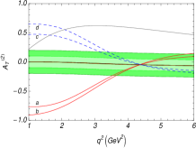
    AT2superscriptsubscript𝐴𝑇2A_{T}^{2} is sensitive to both the modulus and sign of C7eff⁣′subscriptsuperscript𝐢effβ€²7C^{{\rm eff}\prime}_{7}, being approximately zero in the SM. This sensitivity is enhanced by a factor 4​mb​MB/q24subscriptπ‘šπ‘subscript𝑀𝐡superscriptπ‘ž24m_{b}M_{B}/q^{2} at low q2superscriptπ‘ž2q^{2} (q2∼1​GeV2similar-tosuperscriptπ‘ž21superscriptGeV2q^{2}\sim 1\,{\rm GeV}^{2}), and for larger values of q2superscriptπ‘ž2q^{2} (1<q2<4​GeV21superscriptπ‘ž24superscriptGeV21<q^{2}<4\,{\rm GeV}^{2}) the observable decreases with a 1/s1𝑠1/s slope. This is clearly shown in Fig.1 looking at the curves, a,b,c and d.

  • β€’

    Finally AT2superscriptsubscript𝐴𝑇2A_{T}^{2} exhibits a zero, at the point Ξ”βˆ’+Ξ”+βˆ—=0subscriptΞ”superscriptsubscriptΞ”0\Delta_{-}+\Delta_{+}^{*}=0 corresponding exactly to the zero of the FB asymmetry at LO. Being this zero independent of C7eff⁣′subscriptsuperscript𝐢effβ€²7C^{{\rm eff}\prime}_{7}, all curves with SM-like C7subscript𝐢7C_{7} should exhibit it (see Fig.1). Finally it was shown in [6] that contrary to the case of AT2superscriptsubscript𝐴𝑇2A_{T}^{2} the observable AF​Bsubscript𝐴𝐹𝐡A_{FB} does not show any remarkable sensitivity to the presence of RH currents. This stress the importance of AT2superscriptsubscript𝐴𝑇2A_{T}^{2} as one of the best indicators of the presence of this type of NP.

In summary AT2superscriptsubscript𝐴𝑇2A_{T}^{2} provides different informations depending on the region of q2superscriptπ‘ž2q^{2} analyzed: at low q2superscriptπ‘ž2q^{2} (q2∼1​GeV2similar-tosuperscriptπ‘ž21superscriptGeV2q^{2}\sim 1\,{\rm GeV}^{2}) basically sets the size of the coefficient C7eff⁣′subscriptsuperscript𝐢effβ€²7C^{{\rm eff}\prime}_{7} and at high q2superscriptπ‘ž2q^{2} (q2∼4​GeV2similar-tosuperscriptπ‘ž24superscriptGeV2q^{2}\sim 4\rm\,GeV^{2}) behaves as the FB asymmetry, with a zero in the energy axis. This last point implies obviously, that in case of a flipped sign solution for C7effsuperscriptsubscript𝐢7effC_{7}^{\rm eff} the behaviour of AT2superscriptsubscript𝐴𝑇2A_{T}^{2} will change drastically. This is shown by the grey curve in Fig.1a that does not have a zero, like in the FB asymmetry. In this sense AT2superscriptsubscript𝐴𝑇2A_{T}^{2} goes beyond the AF​Bsubscript𝐴𝐹𝐡A_{FB} because it contains the most important features of this observable and also show up a dramatic dependence on the presence of RH currents (O7β€²superscriptsubscript𝑂7β€²O_{7}^{\prime}) invisible to AF​Bsubscript𝐴𝐹𝐡A_{FB}.

Refer to caption
Refer to caption
Refer to caption
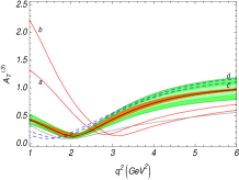
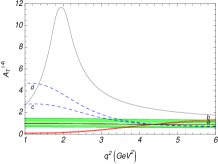
Figure 1: AT2superscriptsubscript𝐴𝑇2A_{T}^{2} (a), AT3superscriptsubscript𝐴𝑇3A_{T}^{3}(b) and AT4superscriptsubscript𝐴𝑇4A_{T}^{4}(c) in SM and SUSY (curves a,b,c,d). The outer dark and light (green) bands are, respectively, the possible 5 and 10% Ξ›/mbΞ›subscriptπ‘šπ‘\Lambda/m_{b} corrections to the amplitudes, varied independently for each amplitude and added in quadrature. The inner (orange) band around the SM prediction (black curve) contains the hadronic and renormalisation scale uncertainties, also added in quadrature. The grey curve corresponds to the flipped sign solution (C7eff,C7eff⁣′)=(0.04,0.31).subscriptsuperscript𝐢eff7subscriptsuperscript𝐢effβ€²70.040.31(C^{\rm{eff}}_{7},C^{\rm{eff}\prime}_{7})=(0.04,0.31).

A similar exercise can be done with the observables AT3superscriptsubscript𝐴𝑇3A_{T}^{3} and AT4superscriptsubscript𝐴𝑇4A_{T}^{4} [6]. Those are particularly interesting because they open the sensitivity to the longitudinal spin amplitude A0subscript𝐴0A_{0} minimizing, at the same time, the sensitivity to the other soft form factor ΞΎβˆ₯​(0)subscriptπœ‰βˆ₯0\xi_{\|}(0).

Both can be very easily measured from the angular distribution and their explicit form in the heavy quark and large-EKβˆ—subscript𝐸superscript𝐾E_{K^{*}} limit for the spin amplitudes, even if less iluminating, still shows clearly the different way they depend on the RH currents. They are:

AT3=|A0​L​Aβˆ₯Lβˆ—+A0​Rβˆ—β€‹Aβˆ₯R||A0|2​|AβŸ‚|2\displaystyle A_{T}^{{3}}\!=\!\frac{|A_{0L}A_{\|L}^{*}+A_{0R}^{*}A_{\|R}|}{\sqrt{|A_{0}|^{2}|A_{\perp}|^{2}}} ∼similar-to\displaystyle\!\!\sim\!\! q2​(Ξ”~βˆ’+f1)+Ξ”~βˆ’β€‹(f2+Ξ”~βˆ’β€‹f3)f4​Δ~βˆ’2+f5​Δ~βˆ’+f6​Δ~+​q2+f7​q4+f8​Δ~+2superscriptπ‘ž2superscript~Ξ”subscript𝑓1superscript~Ξ”subscript𝑓2superscript~Ξ”subscript𝑓3subscript𝑓4superscript~Ξ”2subscript𝑓5superscript~Ξ”subscript𝑓6superscript~Ξ”superscriptπ‘ž2subscript𝑓7superscriptπ‘ž4subscript𝑓8superscript~Ξ”2\displaystyle\frac{q^{2}\left({\tilde{\Delta}^{-}}+f_{1}\right)+{\tilde{\Delta}^{-}}\left(f_{2}+{\tilde{\Delta}^{-}}f_{3}\right)}{\sqrt{f_{4}{\tilde{\Delta}}^{-2}+f_{5}{\tilde{\Delta}}^{-}+f_{6}}\sqrt{{\tilde{\Delta}}^{+}q^{2}+f_{7}q^{4}+f_{8}{\tilde{\Delta}}^{+2}}}\,
AT4=|A0​L​AβŸ‚Lβˆ—βˆ’A0​Rβˆ—β€‹AβŸ‚R||A0​L​Aβˆ₯Lβˆ—+A0​Rβˆ—β€‹Aβˆ₯R|\displaystyle A_{T}^{{4}}\!=\!\frac{|A_{0L}A_{\perp L}^{*}-A_{0R}^{*}A_{\perp R}|}{|A_{0L}A_{\|L}^{*}+A_{0R}^{*}A_{\|R}|} ∼similar-to\displaystyle\!\!\sim\!\! f9​Δ~++q2​(f10​Δ~βˆ’+f11)q2​(Ξ”~βˆ’+f1)+Ξ”~βˆ’β€‹(f2+Ξ”~βˆ’β€‹f3)subscript𝑓9superscript~Ξ”superscriptπ‘ž2subscript𝑓10superscript~Ξ”subscript𝑓11superscriptπ‘ž2superscript~Ξ”subscript𝑓1superscript~Ξ”subscript𝑓2superscript~Ξ”subscript𝑓3\displaystyle\frac{f_{9}{\tilde{\Delta}}^{+}+q^{2}\left(f_{10}{\tilde{\Delta}}^{-}+f_{11}\right)}{q^{2}\left({\tilde{\Delta}^{-}}+f_{1}\right)+{\tilde{\Delta}^{-}}\left(f_{2}+{\tilde{\Delta}^{-}}f_{3}\right)}\,

where fi=f​(π’ž9eff,C10)subscript𝑓𝑖𝑓superscriptsubscriptπ’ž9effsubscript𝐢10f_{i}=f({\cal C}_{9}^{\rm eff},C_{10}) with i=1,..11𝑖1..11i=1,..11 [7] are simple functions of these coefficients and Ξ”~Β±=C7effΒ±C7eff⁣′superscript~Ξ”plus-or-minusplus-or-minussubscriptsuperscript𝐢eff7subscriptsuperscript𝐢effβ€²7{{\tilde{\Delta}}^{\pm}={C^{{\rm eff}}_{7}}\pm{C^{{\rm eff}\prime}_{7}}}. Here a small weak phase has been neglected. As can be seen from their defining expressions and from the Figs. 1b-1c, AT3superscriptsubscript𝐴𝑇3A_{T}^{3} and AT4superscriptsubscript𝐴𝑇4A_{T}^{4} play a complementary role, where AT3superscriptsubscript𝐴𝑇3A_{T}^{3} shows a minimum AT4superscriptsubscript𝐴𝑇4A_{T}^{4} has a maximum, and viceversa. For example, in the specific SUSY cases discussed, it is clear from Figs. 1a-1b that the low-gluino scenario with negative mass insertion is clearly enhanced in the low-q2superscriptπ‘ž2q^{2} region for AT4superscriptsubscript𝐴𝑇4A_{T}^{4}, while the large-gluino scenario with positive mass insertion is clearly signaled in the low-q2superscriptπ‘ž2q^{2} region for AT3superscriptsubscript𝐴𝑇3A_{T}^{3} and in the large-q2superscriptπ‘ž2q^{2} region for AT4superscriptsubscript𝐴𝑇4A_{T}^{4}. Finally, from the set of functions fisubscript𝑓𝑖f_{i}[7] it is easy at LO to obtain with good precision the position of the maxima/minima. The way the sensitivity to RH currents is manifested is through the position of the maxima/minima in AT3superscriptsubscript𝐴𝑇3A_{T}^{3} and AT4superscriptsubscript𝐴𝑇4A_{T}^{4}. In the case of the flipped sign solution (grey curve of Fig. 1) this is shown also by the position of more prominent peak in AT4superscriptsubscript𝐴𝑇4A_{T}^{4} (as seen in Fig 1c).

The same philosophy as in [6] can be applied to CP violating observables (see [7, 11] for a detailed discussion). Finally the excellent experimental sensitivity at LHCb specially for AT2superscriptsubscript𝐴𝑇2A_{T}^{2} from a full angular analysis will allow to disentangle cleanly the presence of RH currents [6, 7, 12].

Acknowledgments: JM and MR acknowledge financial support from FPA2008-01430 and MRTN-CT-2006-035482 and also from UAB, UE and WR from STFC, TH acknowledges financial support from Heptools and the ITP of the University Zurich.

References

  • [1] A.Β Ali, T.Β Mannel and T.Β Morozumi, Phys.Β Lett.Β  B 273 (1991) 505.
  • [2] M.Β Beneke, T.Β Feldmann and D.Β Seidel, Nucl.Β Phys.Β  B 612 (2001) 25
  • [3] T.Β Feldmann and J.Β Matias, JHEP 0301 (2003) 074
  • [4] F.Β Kruger and J.Β Matias, Phys.Β Rev.Β  D 71 (2005) 094009
  • [5] E.Β Lunghi and J.Β Matias, JHEP 0704 (2007) 058
  • [6] U.Β Egede, T.Β Hurth, J.Β Matias, M.Β Ramon, W.Β Reece, JHEP 0811 (2008) 032
  • [7] U.Β Egede, T.Β Hurth, J.Β Matias, M.Β Ramon, W.Β Reece, in preparation.
  • [8] W.Β Altmannshofer, P.Β Ball, A.Β Bharucha, A.Β J.Β Buras, D.Β M.Β Straub and M.Β Wick, JHEP 0901 (2009) 019
  • [9] C.Β Bobeth, G.Β Hiller and G.Β Piranishvili, JHEP 0807 (2008) 106
  • [10] J.Β Charles et al., Phys.Β Rev.Β  D 60 (1999) 014001
  • [11] U. Egede, T. Hurth, J. Matias, M. Ramon, W. Reece, talk at EPS conference,
    β€œNew physics reach of CP violating observables in the decay Bdβ†’Kβˆ—β€‹l+​lβˆ’β†’subscript𝐡𝑑superscript𝐾superscript𝑙superscript𝑙B_{d}\to K^{*}l^{+}l^{-} ”, Krakow, Poland, July 2009, [arXiv:0912.1349 [hep-ph]].
  • [12] W. Reece for the LHCb collaboration, talk at Beauty conference,
    β€œBdβ†’Kβˆ—β€‹ΞΌβ€‹ΞΌβ†’subscript𝐡𝑑superscriptπΎπœ‡πœ‡B_{d}\to K^{*}\mu\mu at LHCb”, Heidelberg, Germany, 2009.