Chiral Generations on Intersecting 5-branes
in Heterotic String Theory

Abstract

We show that there exist two 27 and one $\overline{\bf 27}$ of $E_{6}$, net one $D=4$, ${\cal N}=1$ chiral matter supermultiplet as zero modes localized on the intersection of two 5-branes in the $E_{8}\times E_{8}$ heterotic string theory. The smeared intersecting 5-brane solution is used via the standard embedding to construct a heterotic background, which provides, after a compactification of some of the transverse dimensions, a five-dimensional Randall-Sundrum II like brane-world set-up in heterotic string theory. As a by-product, we present a new proof of anomaly cancellation between those from the chiral matter and the anomaly inflow onto the brane without small instanton.

I Introduction

How the Standard Model emerges in string theory is a long-standing question. In early days of string theory, the heterotic string theory heterotic_string was considered as a promising candidate for the fundamental theory which would provide a basis for model building. Its miraculous anomaly cancellation allows only two choices (that is, $E_{8}\times E_{8}$ and $SO(32)$) of a consistent gauge group, and in Calabi-Yau compactifications (including orbifold and other $1/4$ supersymmetric compactifications in a broad sense) there appear variety of four-dimensional supersymmetric standard-model-like theories with chiral generations. The problem is, however, that the number of such possible compactifications seems too large Susskind to find natural necessity for our world to be as observed, despite the remarkable uniqueness of the original theory.

In the late last century, a conceptually different approach was proposed to realize a four-dimensional world by using D-branes in type II string theories. The key observation is that two intersecting D-branes can support chiral fermions at the intersection BDL . Since then many intersecting D-brane models have been built and discussed so far. We refer to the articles IntersectingDbraneModels for a review of these developments. Also, inspired by the discovery of D-branes, brane-world models have also been extensively studied as a possible solution to the hierarchy problem and in terms of cosmological model building ADD ; RS1 ; RS2 .

In this paper, we propose a new brane-world set-up for $E_{6}$ GUT model building by using intersecting 5-branes in heterotic string theory. The 5-branes in heterotic string theory are, of course, not D-branes. They are NS5-branes SJR ; Strominger , and unlike D-branes, they are not described by open strings. What makes them hard to deal with is that, near the core of the solution, the geometry is not AdS but an infinite throat where the dilaton diverges linearly. Nevertheless, we can identify what low-energy excitations are on the brane by investigating zero modes of the supergravity solution CHS . It has been known for some time that on a symmetric 5-brane CHS there are 30 $D=6$, ${\cal N}=1$ supermultiplet as zero modes in either of $E_{8}\times E_{8}$ or $SO(32)$ heterotic string theory. In fact, as we explain in section II, they can be regarded as certain Nambu-Goldstone modes associated with various spontaneously broken symmetries of the theory. Therefore, we may expect that, as pions are effectively described by the chiral model without detailed knowledge of QCD, the zero modes on the heterotic 5-branes may also provide enough information for low-energy model building, even though their microscopic description (such as little string theory) is not fully understood. The existence of chiral zero modes is also consistent with the anomaly cancellation against an anomaly inflow from the bulk.

In order to examine the zero modes on the intersecting system, we first construct an intersecting 5-brane solution in the $E_{8}\times E_{8}$ heterotic string theory by the so-called standard embedding in the known smeared intersecting NS5-brane solution of type II theories. We then study the zero modes of the relevant Dirac operator on this background. We show that there exist three localized chiral zero modes, two of which are in the 27 representation of $E_{6}$, and one in the $\overline{\bf 27}$ representation. They give rise to net one 27 of massless chiral fermions in the four-dimensional spacetime. Therefore, still being a toy model, this is the first example of a brane set-up in heterotic string theory that supports four-dimensional chiral matter fermions transforming as an $E_{6}$ gauge multiplet .

There is a good reason why we should study NS5-branes as a set-up for particle-physics model building: They are T-dual to noncompact Calabi-Yau manifolds obtained by blowing up an isolated singularity T-dual . For instance, parallel NS5-branes are known to be T-dual to a multi-center Taub-NUT, or an $A_{n}$ singularity which is obtained as a limit of a Taub-NUT. Similarly, a system of two intersecting 5-branes is known to be T-dual to a deformed conifold conifold . Therefore, the intersecting 5-brane background in heterotic string theory may be regarded as a T-dual to a heterotic “compactification” on the deformed conifold. While there are a variety of compact Calabi-Yau manifolds with complicated structures, singularities may occur on a moduli space of any compact Calabi-Yau, and the local structure of a singularity is universal and can be simple, no matter what the rest of the manifold is. Therefore, the idea is that if a realistic GUT could be realized on such a singularity, it would mean that our universe is not just a coincidence, as every compact Calabi-Yau has a chance to realize the GUT on a part of it.

This work is a first step toward a brane realization of a realistic $E_{6}$ GUT model in string theory. The remainder of this paper is organized as follows: In section II, we give a brief review of known 5-brane solutions in type II and heterotic supergravity theories. In section III, we present a new proof of anomaly cancellation between those from the chiral matter on the brane and the anomaly inflow into the brane in the $E_{8}\times E_{8}$ heterotic theory. In section IV, we construct an intersecting solution in the heterotic theory, and compute explicitly the zero modes of the Dirac operator to find net $2-1=1$ set of chiral zero modes transforming as the 27 representation of $E_{6}$. The last section is devoted to conclusions and discussion.

II Review of 5-brane Solutions in Heterotic String Theory

We will focus on the $E_{8}\times E_{8}$ heterotic string theory. The string-frame bosonic supergravity Lagrangian is given, to $O(\alpha^{\prime})$ BdR ; KY , as

$${\cal L} = \frac{1}{2\kappa^{2}}\int d^{10}x\sqrt{-g}e^{-2\phi}\left\{R(\omega)-\frac{1}{3}H_{MNP}H^{MNP}+4(\partial_{M}\phi)^{2}\right.$$ (1)

$$\left.\hskip 113.81102pt-\alpha^{\prime}\left(\frac{1}{30}\text{Tr}(F_{MN}F^{MN})-R_{MNAB}(\omega_{+})R^{MNBA}(\omega_{+})\right)\right\}.$$

The convention we use in this paper is basically the one used in Callan-Harvey-Strominger’s original paper CHS , and KY , to which the reader is also referred for the comparison with other articles such as BdR .

As already seen in the above effective Lagrangian, particular combinations of the spin connection $\omega$ and the antisymmetric three-form $H$ play different roles in different places BdR ; KY . In (1), the $R^{2}$ term is the Riemann square made of the combination

$$\omega_{+} \equiv \omega+H.$$ (2)

This combination also appears in the higher order terms in the effective action, and in the Bianchi identity for the $H$ field in the presence of flux:

$$dH = \alpha^{\prime}\left(\text{tr}(R(\omega_{+})\wedge R(\omega_{+}))-\frac{1}{30}\text{Tr}(F\wedge F)\right).$$ (3)

On the other hand, another combination

$$\omega_{-} \equiv \omega-H$$ (4)

is relevant for the lowest order SUSY variation of the gravitino:

$$\delta\psi_{M} = \left(\partial_{M}+\frac{1}{4}\omega_{-M}{}^{AB}\Gamma_{AB}\right)\epsilon.$$ (5)

Finally, the Dirac operator of the gaugino equation of motion has a combination $\omega-\frac{1}{3}H$ as will be seen in a moment. The relations among the above three spin connections are discussed in TK0704 .

II.1 The neutral solution

In the absence of the nonabelian gauge field, the following configurations solve the leading order equations of motion:

$$g_{ij} = \eta_{ij}~{}~{}~{}(i,j=0,1,\ldots,5),$$

$$g_{\mu\nu} = e^{2\phi}\delta_{\mu\nu}~{}~{}~{}(\mu,\nu=6,\ldots,9),$$

$$e^{2\phi} = e^{2\phi_{0}}+\frac{n\alpha^{\prime}}{x^{2}},$$

$$H_{\mu\nu\lambda} = -\epsilon_{\mu\nu\lambda}{}^{\rho}\partial_{\rho}\phi,$$ (6)

where

$$x^{2}\equiv\sum_{\mu=6}^{9}(x^{\mu})^{2}.$$ (7)

$\epsilon^{\mu\nu\lambda\rho}$ is the (undensitized) completely antisymmetric tensor. All other components of $H$ vanish.

The solution (6) may be regarded as representing the NS5-branes stacked on top of each other in both type IIA and type IIB theories. It has a nonzero axion charge

$$\frac{1}{2\pi^{2}}\int_{S^{3}}H = n\alpha^{\prime}.$$ (8)

$n$ must be an integer. This is an everywhere smooth solution; $x=0$ is an apparent singularity as is verified by the coordinate transformation $t\equiv\ln x^{2}$ CHS . The scalar curvature and Riemann square (in the string frame) are both everywhere finite:

$$R = \frac{6}{n\alpha^{\prime}}\cdot\frac{1}{(1+\frac{x^{2}}{\rho^{2}})^{3}},$$ (9)

$$R_{ABCD}R^{ABCD} = \frac{12}{n^{2}{\alpha^{\prime}}^{2}}\cdot\frac{1+4\frac{x^{2}}{\rho^{2}}+8(\frac{x^{2}}{\rho^{2}})^{2}}{(1+\frac{x^{2}}{\rho^{2}})^{6}},$$ (10)

where $\rho^{2}\equiv e^{-2\phi_{0}}n\alpha^{\prime}$. The supergravity analysis is trusted if the string coupling is small enough, and the metric varies slow enough:

$$e^{2\phi}\ll 1,\hskip 14.22636ptR\ll{\alpha^{\prime}}^{-1}.$$ (11)

They are satisfied if

$$e^{2\phi_{0}}\ll 1,\hskip 14.22636pt\rho\ll|x|.$$ (12)

When considered in heterotic string theory later, the parameter $\rho$ corresponds to the size of the instanton. Therefore, a small instanton means that the string coupling is everywhere large, and some nonperturbative phenomenon is known to occur small_instanton . Even though $e^{-\phi_{0}}$ is large, the dilaton becomes large if one gets closer than the instanton size to the brane. However, a close relative of the symmetric 5-brane has been obtained GiddingsStrominger as a certain double scaling limit of a non-extremal solution, and it is known to have, as a part of its near-horizon geometry, a two-dimensional black hole rather than a linear-dilaton throat geometry. CFT models inspired by this solution have been constructed noncompactGepner . (The worldsheet approach for 5-branes was originally mentioned in the second reference of SJR .)

The zero modes on this solution are a six-dimensional chiral $(2,0)$ matter supermultiplet in the IIA case, and nonchiral $(1,1)$ supermultiplet in the IIB case CHS . This flip of the chirality may be understood as a consequence of the T-duality to the ADE singularities.

II.2 The symmetric solution

Next we include a nonabelian gauge field in heterotic string theory. It is well known that in order for the anomaly cancellation mechanism to work, the Bianchi identity must be modified as we saw in (3) as to

$$dH = \alpha^{\prime}\left(\text{tr}(R(\omega_{+})\wedge R(\omega_{+}))-\frac{1}{30}\text{Tr}(F\wedge F)\right),$$ (13)

where Tr is the trace in the adjoint representation of $E_{8}\times E_{8}$ or $SO(32)$.

Since the neutral solution satisfies $dH=0$ except at the brane position $x^{\mu}=0$ where the magnetic 5-brane charge is located, it remains a solution in heterotic theory only if the right hand side vanishes. The most common way to achieve this is to set $\omega_{+}$ equal to the gauge connection $A$. This may be called the “standard” embedding, but the point is that, in the presence of nonzero $H$ flux, what is embedded in the gauge connection is not simply the spin connection $\omega$, but the particular combination $\omega+H$. What is nice about this embedding is that some corrections of the supersymmetry variations to higher orders in $\alpha^{\prime}$ vanish BdR .

The spin connections computed in the neutral background (6) are found to be

$$\omega_{\mu}{}^{\alpha}{}_{\beta} = (\delta_{\mu}^{\alpha}\delta_{\beta}^{\nu}-\delta_{\mu\beta}\delta^{\alpha\nu})\partial_{\nu}\phi.$$ (14)

All other components vanish. The $H$ field is written as

$$H_{\mu}{}^{\alpha}{}_{\beta} = -\epsilon^{\alpha}{}_{\beta}{}^{\gamma\delta}\,\delta_{\mu\gamma}\delta_{\delta}^{~{}\nu}\partial_{\nu}\phi.$$ (15)

Therefore $\omega_{+}$ is given by

$$\omega_{+\mu}{}^{\alpha\beta} \equiv (\omega+H)_{\mu}{}^{\alpha\beta}$$ (16)

$$= 2\rho^{2}\sigma^{\alpha\beta}{}_{\mu\lambda}\cdot\frac{x^{\lambda}}{x^{2}(x^{2}+\rho^{2})},$$

where

$$\sigma^{\alpha\beta}{}_{\mu\lambda} \equiv \delta_{\mu}^{\alpha}\delta_{\lambda}^{\beta}-\frac{1}{2}\epsilon^{\alpha\beta}{}_{\gamma\delta}\,\delta_{\mu}^{\gamma}\delta_{\lambda}^{\delta},$$ (17)

$$\rho^{2} \equiv e^{-2\phi_{0}}n\alpha^{\prime}.$$ (18)

The tensor $\sigma^{\alpha\beta}{}_{\mu\lambda}$ is anti-self-dual:

$$\frac{1}{2}\epsilon^{\alpha\beta}{}_{\gamma\delta}\,\sigma^{\gamma\delta}{}_{\mu\nu} = -\sigma^{\alpha\beta}{}_{\mu\nu}.$$ (19)

Thus the $SO(4)$ connection $\omega_{+}$ is anti-self-dual, which means that the structure group of the bundle is reduced to $SU(2)$. We then identify

$$A_{\mu}^{\alpha\beta} = \omega_{+\mu}{}^{\alpha\beta},$$ (20)

and assume all other components to be zero. This is the symmetric solution CHS . In this way, a part of the gauge connection acquires a nonzero background in an $SU(2)$ subalgebra of $E_{8}\times E_{8}$.

This is a supersymmetric configuration; a different combination

$$\omega_{-\mu}{}^{\alpha\beta} \equiv (\omega-H)_{\mu}{}^{\alpha\beta}$$ (21)

$$= 2\rho^{2}\hat{\sigma}^{\alpha\beta}{}_{\mu\lambda}\cdot\frac{x^{\lambda}}{x^{2}(x^{2}+\rho^{2})},$$

$$\hat{\sigma}^{\alpha\beta}{}_{\mu\lambda} \equiv \delta_{\mu}^{\alpha}\delta_{\lambda}^{\beta}+\frac{1}{2}\epsilon^{\alpha\beta}{}_{\gamma\delta}\,\delta_{\mu}^{\gamma}\delta_{\lambda}^{\delta}$$

is a self-dual connection, and hence belongs also to a (different) $SU(2)$ subalgebra of $SO(4)$. This ensures that there is a Killing spinor for the gravitino SUSY variation

$$\delta\psi_{M} = \left(\partial_{M}+\frac{1}{4}\omega_{-M}{}^{AB}\Gamma_{AB}\right)\epsilon.$$ (22)

On the other hand, the gaugino SUSY variation reads

$$\delta\chi^{\alpha\beta} = -\frac{1}{4}\Gamma^{MN}F_{MN}^{\alpha\beta}\epsilon,$$ (23)

where the $SO(4)$ matrix indices $\alpha,\beta$ are now understood as the $SU(2)$ gauge indices. The field strength $F_{MN}^{\alpha\beta}$ involves the connection $\omega_{+}$ due to the embedding, and not $\omega_{-}$. However, there is a following identity between the Riemann tensor made of the connection $\omega_{+}$ and that made of $\omega_{-}$:

$$R(\omega_{+})_{MNPQ} = R(\omega_{-})_{PQMN}+(dH)_{MNPQ}.$$ (24)

Therefore, in the background where $dH$ vanishes, the gaugino variation (23) amounts to

$$\delta\chi^{\alpha\beta} = -\frac{1}{4}\Gamma^{\mu\nu}F_{\mu\nu}^{\alpha\beta}\epsilon$$ (25)

$$= -\frac{1}{4}\Gamma^{\mu\nu}R(\omega_{+})_{\mu\nu}{}^{\alpha\beta}\epsilon$$

$$= -\frac{1}{4}\Gamma^{\gamma\delta}R(\omega_{-})^{\alpha\beta}{}_{\gamma\delta}\epsilon.$$

Thus the Killing spinor $\epsilon$ for the gravitino variation (22) is automatically the Killing spinor for the gaugino variation (23). (The dilatino variation equation must be checked separately.) The $SU(2)$ gauge connection $A_{\mu}^{\alpha\beta}$ (20) satisfies the lowest-order equation of motion

$$\partial_{\nu}\left(\sqrt{-g}e^{-2\phi}F^{\mu\nu\alpha\beta}\right)+\sqrt{-g}e^{-2\phi}\left({[}A_{\nu},~{}F^{\mu\nu}{]}^{\alpha\beta}-H^{\mu\nu\rho}F_{\nu\rho}^{\alpha\beta}\right) = 0$$ (26)

as expected.

II.3 Zero modes on the symmetric 5-brane

Let us consider zero modes existing on the symmetric 5-brane solution (6) with (20) CHS . The obvious bosonic zero modes are the four translation moduli, and the instanton size $\rho$ modulus. Besides, there are other zero modes coming from infinitesimal global gauge rotations of the instanton: By construction, the gauge fields have nonzero vacuum expectation values in the four-dimensional space transverse to the 5-brane. They belong to an $SU(2)$ subalgebra of one of $E_{8}$. The centralizer of $SU(2)$ in $E_{8}$ is $E_{7}$, and the adjoint 248 is decomposed into a sum of representations of $E_{7}\times SU(2)$ as

$${\bf 248} = ({\bf 133},{\bf 1})\oplus({\bf 56},{\bf 2})\oplus({\bf 1},{\bf 3}).$$ (27)

133, the adjoint of $E_{7}$, does nothing on the $SU(2)$ background, while the other $56\times 2+1\times 3=115$ generators rotate the background, and hence give rise to zero modes. Thus, in all, there are $4+1+115=120$ bosonic zero modes on this background. Since the symmetric solution is half BPS, they together with their superpartners constitute 30 $D=6$, ${\cal N}=1$ hypermultiplets. The existence of the fermionic zero modes have also been confirmed by the index theorem Bellisai .

These zero modes can be regarded as Nambu-Goldstone modes associated with various spontaneously broken symmetries of the theory HughesPolchinski . Indeed, the four position moduli above are the Nambu-Goldstone modes coming from the spontaneous broken translational invariance due to the presence of the 5-brane. The size modulus corresponds to the broken scale invariance. The remaining $115$ moduli are also thought of as coming from how the $SU(2)$ subalgebra is embedded in the whole $E_{8}$ Lie algebra; by “standard embedding” we mean we choose some $SU(2)$ in $E_{8}$ and set the gauge connection for this $SU(2)$ to be equal to the (generalized) spin connection. But the choice of such an $SU(2)$ is arbitrary, and the original $E_{8}$ symmetry is spontaneously broken. Incidentally, this way of counting reproduces the correct instanton-number dependence of the dimensions of instanton moduli in flat space, for all gauge groups, obtained by the index theorem BCGW .

But there is a puzzle here: Why aren’t they absorbed into the gauge bosons by the Higgs mechanism? The gauge bosons in the transverse dimensions can be viewed as adjoint Higgs fields from the brane, and the standard embedding amounts to giving vev’s to these Higgs fields. Then small fluctuations around the vev’s are Nambu-Goldstone modes, which are completely gauged away to leave, in ordinary gauge theories, a Proca Lagrangian for massive vector fields. This is the standard Higgs mechanism in the textbook, and it is interpreted to mean that the Nambu-Goldstone modes are “eaten” by the gauge bosons to be their longitudinal degrees of freedom. So why are there such extra zero-mode degrees of freedom left on the brane, other than those used as a part of massive vector bosons in the bulk?

The resolution to this problem lies in the apparent breakdown of the gauge invariance due to the Green-Schwarz counterterm $BX_{8}\sim-dBX_{7}$. In eliminating the small fluctuations around the vev, both $B$ and $X_{7}$ also get transformed by the gauge transformation. The contribution from the variation of $B$ is compensated by the one-loop anomaly in the bulk GSmechanism , while that from $X_{7}$ vanishes if there are no magnetic source of the $B$ field $d^{2}B=0$. In the present case, however, there is such a source $d^{2}B\propto\delta^{4}(x^{\mu})$, and therefore the gauge variation of $X_{7}$ gives rise to a change of the field configurations on the brane. Thus gauge transformations can not completely eliminate the fluctuations of the “Higgs”, but local fluctuations are left on the brane .

This phenomenon is known as anomaly inflow anomaly_inflow , and the change of the brane action is cancelled by, again, the one-loop effect of chiral fermions on the brane, which are the superpartners of the bosonic zero modes. The gauge invariance of the total quantum action is thus restored. In the next section, we will show the precise arithmetic of the cancellation.

III Anomaly Inflow and Cancellation

We will show that the 30 hypermultiplets, 28 (=56 half-hypermultiplets) in the 56 representation of $E_{7}$ and two singlets (=4 half-hypermultiplets), precisely cancel the inflows of the tangent bundle, $E_{7}$ gauge and mixed anomalies via the Green-Schwarz mechanism. The cancellation of anomalies on the gauge 5-brane CHS in heterotic string theory was already discussed in BlumHarvey . Here we give a somewhat different proof of cancellation than theirs in the case of the $E_{8}\times E_{8}$ symmetric 5-brane. Although they should be basically the same, ours is closely parallel to Mourad Mourad and appears to be simpler. In particular, we do not need to consider any current at infinity. We ignore the normal bundle connection and write out only terms consisting of the tangent bundle and gauge connections.

The relevant anomaly polynomials are

$$I_{8}^{singlet} = \left.\frac{1}{2}\hat{A}(T\Sigma)\right|_{8}\times 4$$ (28)

$$= \frac{2}{5760}(-4p_{2}+7p_{1}^{2}),$$

$$I_{8}^{\bf 56} = \left.\frac{1}{2}\hat{A}(T\Sigma)\mbox{tr}_{\bf 56}e^{iF}\right|_{8}$$ (29)

$$= \frac{28}{5760}(-4p_{2}+7p_{1}^{2})+\frac{1}{96}p_{1}^{2}\mbox{tr}_{\bf 56}F^{2}+\frac{1}{48}\mbox{tr}_{\bf 56}F^{4},$$

and

$$X_{8} = \frac{1}{24}\left(\frac{1}{8}\mbox{tr}R^{4}+\frac{1}{32}(\mbox{tr}R^{2})^{2}-\frac{1}{240}\mbox{tr}R^{2}\mbox{Tr}_{\bf 248}F^{2}+\frac{1}{24}\mbox{Tr}_{\bf 248}F^{4}-\frac{1}{7200}(\mbox{Tr}_{\bf 248}F^{2})^{2}\right)$$ (30)

$$= \frac{1}{192}(-4p_{2}+7p_{1}^{2})+\frac{1}{2880}p_{1}^{2}\mbox{Tr}_{\bf 248}F^{2}+\frac{1}{576}\mbox{Tr}_{\bf 248}F^{4}-\frac{1}{24\cdot 7200}(\mbox{Tr}_{\bf 248}F^{2})^{2}.$$

Since the gauge symmetry is broken from $E_{8}$ to $E_{7}$, we rewrite the traces in the representations of $E_{8}$ to those of $E_{7}$. The following formulas are useful Erler :

$$\mbox{Tr}_{\bf 248}F^{2} = (\mbox{Tr}_{\bf 133}+2\mbox{tr}_{\bf 56})F^{2}$$ (31)

$$= 5\mbox{tr}_{\bf 56}F^{2},$$

$$\mbox{Tr}_{\bf 248}F^{4} = (\mbox{Tr}_{\bf 133}+2\mbox{tr}_{\bf 56})F^{4}$$ (32)

$$= \frac{1}{4}(\mbox{tr}_{\bf 56}F^{2})^{2}.$$

$$\mbox{Tr}_{\bf 133}F^{2} = 3\mbox{tr}_{\bf 56}F^{2},$$

$$\mbox{Tr}_{\bf 133}F^{4} = \frac{1}{6}(\mbox{tr}_{\bf 56}F^{2})^{2},$$

$$\mbox{tr}_{\bf 56}F^{4} = \frac{1}{24}(\mbox{tr}_{\bf 56}F^{2})^{2}.$$ (33)

Therefore

$$X_{8} = \frac{1}{192}(-4p_{2}+7p_{1}^{2})+\frac{1}{24^{2}}p_{1}^{2}\mbox{tr}_{\bf 56}F^{2}+\frac{1}{4\cdot 24^{2}}(\mbox{tr}_{\bf 56}F^{2})^{2}-\frac{1}{12\cdot 24^{2}}(\mbox{tr}_{\bf 56}F^{2})^{2}.$$ (34)

They add up to

$$I_{8}^{singlet}+I_{8}^{\bf 56}-X_{8} = \frac{1}{3\cdot 24^{2}}(3p_{1}+\mbox{tr}_{\bf 56}F^{2})(12p_{1}+\mbox{tr}_{\bf 56}F^{2}).$$ (35)

Note that the number (thirty) of hypermultiplets is precisely the one which can cancel out the $p_{2}$ term, otherwise the sum of anomalies does not factorize and the Green-Schwarz mechanism does not apply. Since

$$12p_{1}+\mbox{tr}_{\bf 56}F^{2} = 6\left(-\mbox{tr}R^{2}+\frac{1}{30}\mbox{Tr}_{\bf 248}F^{2}\right),$$ (36)

which is proportional to the anomalous part of the heterotic Bianchi identity, the sum (35) is cancelled by introducing a Green-Schwarz counterterm on the brane as in Mourad .

IV Intersecting 5-branes in Heterotic String Theory

IV.1 Intersecting neutral 5-branes

We will now consider a system of two intersecting NS5-branes. We start with the neutral smeared solution intersecting_solutions :

$$ds^{2} = \sum_{i,j=0,7,8,9}\eta_{ij}dx^{i}dx^{j}+h(x^{1})^{2}\sum_{\mu,\nu=1,2}\delta_{\mu\nu}dx^{\mu}dx^{\nu}+h(x^{1})\sum_{\mu,\nu=3,4,5,6}\delta_{\mu\nu}dx^{\mu}dx^{\nu},$$

$$e^{2\phi} = h(x^{1})^{2},$$

$$H_{\mu\nu\lambda} = \left\{\begin{array}[]{cl}\frac{h^{\prime}}{2}~{}(=\frac{\xi|x^{1}|^{\prime}}{2})&\mbox{if $(\mu,\nu,\lambda)=(2,3,4)$,$(2,5,6)$ or their even permutation},\\ -\frac{h^{\prime}}{2}~{}(=-\frac{\xi|x^{1}|^{\prime}}{2})&\mbox{if $(\mu,\nu,\lambda)=(2,4,3)$,$(2,6,5)$ or their even permutation},\\ 0&\mbox{otherwise,}\end{array}\right.$$ (40)

where

$$h(x^{1})=h_{0}+\xi|x^{1}|.$$ (41)

All other components of $H_{MNL}$ vanish. $h_{0}$ and $\xi$ are real constants. The prime ^′ denotes the differentiation with respect to $x^{1}$, and $|x^{1}|^{\prime}$ is therefore a step function. This is a solution to equations of motion of the leading-order NSNS-sector Lagrangian in type II theories:

$${\cal L}_{NS} = \frac{1}{2\kappa^{2}}\int d^{10}x\sqrt{-g}e^{-2\phi}\left(R(\omega)-\frac{1}{3}H_{MNP}H^{MNP}+4(\partial_{M}\phi)^{2}\right).$$ (42)

The solution describes a pair of intersecting NS5-branes stretching in dimensions as shown in TABLE 1. These branes are delocalized in the $x^{2},x^{3},x^{4},x^{5}$ and $x^{6}$ directions. Consequently, the solution depends only on $x^{1}$, and hence the name “smeared solution”.

Table 1: Dimensions in which the 5-branes stretch.

	0	1	2	3	4	5	6	7	8	9
5-brane1	$\bigcirc$					$\bigcirc$	$\bigcirc$	$\bigcirc$	$\bigcirc$	$\bigcirc$
5-brane2	$\bigcirc$			$\bigcirc$	$\bigcirc$			$\bigcirc$	$\bigcirc$	$\bigcirc$

IV.2 Brane tension and the harmonic function

The coefficient $\xi$ in the definition of the harmonic function $h(x^{1})$ is related to the tension of the brane. To see this, let us consider Einstein’s equation in the Einstein frame:

$$({R_{E}})_{A}{}^{B}-\frac{1}{2}\delta_{A}{}^{B}{R_{E}}-T_{A}{}^{B}=\left\{\begin{array}[]{ll}0&(A,B=1,2),\\ +\frac{h^{\prime\prime}}{2h^{\frac{5}{2}}}&(A,B=3,4,5,6),\\ +\frac{h^{\prime\prime}}{h^{\frac{5}{2}}}&(A,B=0,7,8,9),\end{array}\right.$$ (46)

$$-T_{A}{}^{B}=-\frac{1}{2}\partial_{A}\phi\partial^{B}\phi-e^{-\phi}H_{ACD}H^{BCD}+\frac{1}{2}\delta_{A}^{B}\left(\frac{1}{2}(\partial\phi)^{2}+\frac{1}{3}e^{-\phi}H^{2}\right).$$ (47)

The fact that the right hand side of (46) does not vanish implies that the action must include $\delta$-function like brane-energy terms:

$${\cal L}_{E} = \frac{1}{2\kappa^{2}}\sqrt{-G}R_{E}+{\cal L}_{E}(\phi,H)-V\sqrt{-G_{\text{\scriptsize 5-brane1}}}\prod_{\mu^{\prime}=1,2,3,4}\delta(x^{\mu^{\prime}})$$ (48)

$$~{}~{}~{}~{}~{}~{}~{}~{}~{}~{}~{}~{}~{}~{}~{}~{}~{}~{}~{}~{}~{}~{}~{}~{}~{}~{}~{}~{}~{}~{}~{}-V\sqrt{-G_{\text{\scriptsize 5-brane2}}}\prod_{\mu^{\prime\prime}=1,2,5,6}\delta(x^{\mu^{\prime\prime}}),$$

where $V$ is the brane tension. ${\cal L}_{E}(\phi,H)$ is the Lagrangian for the $\phi$ and $H$ fields in the Einstein frame, which contributes to the energy-momentum tensor $T_{A}{}^{B}$ in (46). The brane metrics are defined as

$${(G_{\text{\scriptsize 5-brane1}})}_{i^{\prime}j^{\prime}} = G_{i^{\prime}j^{\prime}}(x^{\mu^{\prime}}=0)~{}~{}~{}(i^{\prime},j^{\prime}=0,5,6,7,8,9;~{}\mu^{\prime}=1,2,3,4),$$

$${(G_{\text{\scriptsize 5-brane2}})}_{i^{\prime\prime}j^{\prime\prime}} = G_{i^{\prime\prime}j^{\prime\prime}}(x^{\mu^{\prime\prime}}=0)~{}~{}~{}(i^{\prime\prime},j^{\prime\prime}=0,3,4,7,8,9;~{}\mu^{\prime\prime}=1,2,5,6).$$ (49)

What we see here is a no-cosmological-constant analogue of the Randall-Sundrum (RS) models RS1 ; RS2 , and the intersecting nature of the solution is reflected in the two different brane-energy terms. After delocalizations:

$$\prod_{\mu^{\prime}=2,3,4}\delta(x^{\mu^{\prime}}) \rightarrow 1,$$

$$\prod_{\mu^{\prime\prime}=2,5,6}\delta(x^{\mu^{\prime\prime}}) \rightarrow 1,$$ (50)

the inclusion of these terms matches (46) if

$$\xi = -\kappa^{2}Vh_{0}^{\frac{5}{2}}.$$ (51)

Since $e^{\phi}=h(x^{1})$, the sign of $\xi$ strongly affects the dilaton profile. (If $\xi=0$, the solution is reduced to a flat Minkowski space.) We consider the following two cases separately:

Figure 1: $h(x)$ with $\xi>0$. The brane tension is negative. Also, the string coupling becomes stronger as one goes away from the branes.

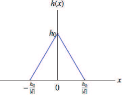
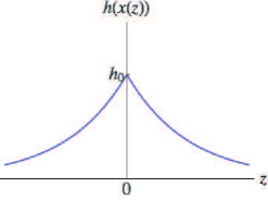
(a)	(b)

Figure 2: $h(x)$ with $\xi<0$. (a) The brane has a positive tension. The string coupling decreases linearly from a positive value $h_{0}$, to necessarily cross the $x^{1}$ axis, where the string coupling becomes zero. We identify this point as the “end of the world”. (b) By a change of the coordinate the points $x=\pm\frac{h_{0}}{|\xi|}$ are mapped to $z=\pm\infty$. The profile of $h(x(z))$ becomes similar to the warp factor of the RS II model.

If $\xi>0$ as in FIG. 1, the brane tension is negative. It is doubtful whether such an object may consistently exist in heterotic string theory. Also, if $\xi>0$, the string coupling becomes stronger as one goes away from the branes, which is puzzling. Thus we consider another option.

If $\xi<0$ as in FIG. 2, the brane has a positive tension. The function $h(x^{1})$, and hence the string coupling, is now convex upwards in $x^{1}$. It decreases linearly from a positive value $h_{0}$, to necessarily cross the $x^{1}$ axis, where the string coupling becomes zero. Beyond that point, $h(x^{1})$ becomes negative, which is inconsistent. Thus we identify this point as the “end of the world”; one can send this point infinitely far away by the coordinate transformation

$$z = -\mbox{sign($x^{1}$)}\log\frac{h(x^{1})}{h_{0}},$$ (52)

where $z$ is the new coordinate. Then the function $h(x^{1})$, which is the string coupling and a typical warp factor for the relatively transverse dimensions, is expressed simply as

$$h = h_{0}~{}e^{-|z|}.$$ (53)

Apparently, this looks similar to the RS II model RS2 , but there are the following differences: The first is that we have no bulk cosmological constant. Instead, we have the dilaton and axion fields (and also the nonabelian gauge fields after the standard embedding) which balance gravity. Secondly, as we see in a moment, there exist chiral zero modes on the branes, which are in the ${\bf 27}$ representation of $E_{6}$. This is not an assumption but a logical consequence of string theory. The final difference is in the warp factor. Unlike the RS models, our four-dimensional metric is not warped at all in the string frame . It would be interesting to examine whether gravity or gauge field is localized, but in this paper we will focus only on the localization of chiral fermions.

IV.3 Intersecting 5-branes in heterotic string theory

We now construct an intersecting solution in the $E_{8}\times E_{8}$ heterotic string theory by the standard embedding, similarly to the previous parallel brane case.

The (generalized) spin connections of the neutral intersecting background are computed as

$$(\omega\pm H)_{\mu=1}{}^{\alpha}{}_{\beta} = 0,$$

$$(\omega\pm H)_{\mu=2}{}^{\alpha}{}_{\beta} = \frac{h^{\prime}}{h}\left(\begin{array}[]{cccccc}&-1&&&&\\ 1&&&&&\\ &&&\pm\frac{1}{2}&&\\ &&\mp\frac{1}{2}&&&\\ &&&&&\pm\frac{1}{2}\\ &&&&\mp\frac{1}{2}&\end{array}\right),$$ (60)

$$(\omega\pm H)_{\mu=3}{}^{\alpha}{}_{\beta} = \frac{h^{\prime}}{2h^{\frac{3}{2}}}\left(\begin{array}[]{cccccc}&&-1&&&\\ &&&\mp 1&&\\ ~{}1&&&&&\\ &\pm 1&&&&\\ &&&&{}{}{}\hfil&\\ &&&&&{}{}{}\hfil\end{array}\right),$$ (67)

$$(\omega\pm H)_{\mu=4}{}^{\alpha}{}_{\beta} = \frac{h^{\prime}}{2h^{\frac{3}{2}}}\left(\begin{array}[]{cccccc}&&&-1&&\\ &&\pm 1&&&\\ &\mp 1&&&&\\ ~{}1&&&&&\\ &&&&{}{}{}\hfil&\\ &&&&&{}{}{}\hfil\end{array}\right),$$ (74)

$$(\omega\pm H)_{\mu=5}{}^{\alpha}{}_{\beta} = \frac{h^{\prime}}{2h^{\frac{3}{2}}}\left(\begin{array}[]{cccccc}&&&&-1&\\ &&&&&\mp 1\\ &&{}{}{}\hfil&&&\\ &&&{}{}{}\hfil&&\\ ~{}1&&&&&\\ &\pm 1&&&&\end{array}\right),$$ (81)

$$(\omega\pm H)_{\mu=6}{}^{\alpha}{}_{\beta} = \frac{h^{\prime}}{2h^{\frac{3}{2}}}\left(\begin{array}[]{cccccc}&&&&&-1\\ &&&&\pm 1&\\ &&&{}{}{}\hfil&&\\ &&{}{}{}\hfil&&&\\ &\mp 1&&&&\\ ~{}1&&&&&\end{array}\right).$$ (88)

The gauge connections are obtained by identifying

$$A_{\mu}^{\alpha\beta} = (\omega+H)_{\mu}^{~{}~{}\alpha\beta}.$$ (89)

The result is

$$A_{\mu=1}^{~{}~{}\alpha\beta} = 0,$$

$$A_{\mu=2}^{~{}~{}\alpha\beta} = \frac{h^{\prime}}{h}\left(\begin{array}[]{ccc}-s&&\\ &\frac{1}{2}s&\\ &&\frac{1}{2}s\end{array}\right)=\frac{h^{\prime}}{h}\left(-\frac{3\lambda_{3}+\sqrt{3}\lambda_{8}}{4}\right)\otimes s,$$ (93)

$$A_{\mu=3}^{~{}~{}\alpha\beta} = \frac{h^{\prime}}{2h^{\frac{3}{2}}}\left(\begin{array}[]{ccc}&-{\bf 1}&\\ {\bf 1}&&\\ &&{}{}{}\hfil\end{array}\right)=\frac{h^{\prime}}{2h^{\frac{3}{2}}}\left(-i\lambda_{2}\right)\otimes{\bf 1},$$ (97)

$$A_{\mu=4}^{~{}~{}\alpha\beta} = \frac{h^{\prime}}{2h^{\frac{3}{2}}}\left(\begin{array}[]{ccc}&-s&\\ -s&&\\ &&{}{}{}\hfil\end{array}\right)=\frac{h^{\prime}}{2h^{\frac{3}{2}}}\left(-\lambda_{1}\right)\otimes s,$$ (101)

$$A_{\mu=5}^{~{}~{}\alpha\beta} = \frac{h^{\prime}}{2h^{\frac{3}{2}}}\left(\begin{array}[]{ccc}&&-{\bf 1}\\ &{}{}{}\hfil&\\ ~{}{\bf 1}&&{}{}{}\hfil\end{array}\right)=\frac{h^{\prime}}{2h^{\frac{3}{2}}}\left(-i\lambda_{5}\right)\otimes{\bf 1},$$ (105)

$$A_{\mu=6}^{~{}~{}\alpha\beta} = \frac{h^{\prime}}{2h^{\frac{3}{2}}}\left(\begin{array}[]{ccc}&&-s\\ &{}{}\hfil&\\ -s&&\end{array}\right)=\frac{h^{\prime}}{2h^{\frac{3}{2}}}\left(-\lambda_{4}\right)\otimes s,$$ (109)

where $\lambda_{i}$’s ($i=1,\ldots,8$) are the Gell-Mann matrices and ${\bf 1}\equiv\left(\begin{array}[]{cc}1&\\ {}{}\hfil&~{}~{}1\end{array}\right)$, $s\equiv i\sigma_{2}=\left(\begin{array}[]{cc}&~{}1\\ -1&\end{array}\right)$.

The explicit expressions (88) show that both of $\omega_{\pm}$ are $SU(3)$ connections. As we did in section II for the symmetric 5-brane, we have embedded $\omega_{+}$ into the gauge connection $A$. Then the Bianchi identity is reduced to $dH=0$, and the solution (40) is consistent with it. This time a certain $SU(3)$ piece of the $E_{8}(\times E_{8})$ gauge connection is given a nonzero expectation value. On the other hand, the fact that $\omega_{-}\in SU(3)$ implies that the Killing spinor equations for the gravitino variation (22) as well as, as explained before, the gaugino variation (22) have a common single Killing spinor. It can be checked that this also satisfies the equation for the dilatino SUSY variation to lowest order:

$$\delta\lambda = \left(-\frac{1}{4}\Gamma^{M}\partial_{M}\phi+\frac{1}{24}\Gamma^{MNP}H_{MNP}\right)\epsilon~{}=0.$$ (110)

Thus the background (40) together with (109) preserve 1/4 of supersymmetries. It also satisfies the equations of motion (26) as it should.

IV.4 Zero modes as Nambu-Goldstone modes on the intersecting 5-branes

In the previous subsection we have constructed a smeared solution which describes intersecting 5-branes in the $E_{8}\times E_{8}$ heterotic string theory to leading order in $\alpha^{\prime}$, via the standard embedding, similarly to the way we obtain the symmetric 5-brane. In that case, the connection $\omega_{+}$ embedded was in $SU(2)$, and the unbroken gauge symmetry was the centralizer $E_{7}$. In the present intersecting case, the connection embedded into $E_{8}$ is in $SU(3)$, and therefore the unbroken gauge symmetry is $E_{6}$. The adjoint representation of $E_{8}$ is decomposed into

$${\bf 248} = ({\bf 78},{\bf 1})\oplus({\bf 27},{\bf 3})\oplus(\overline{\bf 27},\overline{\bf 3})\oplus({\bf 1},{\bf 8})$$ (111)

as representations of the subalgebra $E_{6}\times SU(3)$. Since the $E_{8}\times E_{8}$ gauge field $A_{M}$ has by construction a vev in $SU(3)$, the latter three gauge rotations are the moduli (FIG. 3).

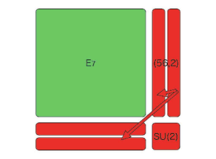
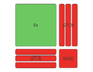
(a)	(b)

Figure 3: Broken generators which give rise to zero modes. (a) The single 5-brane case. (b) The intersecting case.

Let us focus on the $E_{6}$ non-singlet moduli. As we saw in the symmetric 5-brane in the previous sections, spontaneously broken generators in $({\bf 27},{\bf 3})\oplus({\bf\overline{27}},{\bf\overline{3}})$ give rise to Nambu-Goldstone bosons, each of which has one bosonic degree of freedom. On the other hand, since a $D=4$, ${\cal N}=1$ chiral supermultiplet needs two bosonic degrees of freedom, the Nambu-Goldstone bosons which transform as ${\bf 27}$ and ${\bf\overline{27}}$ must be combined to form a single ${\cal N}=1$ chiral supermultiplet. That is, the $E_{6}$ non-singlet moduli form three chiral supermultiplets in the ${\bf 27}$ (or ${\bf\overline{27}}$, but not both) representation of $E_{6}$.

At first sight, one might think that the argument above would be contradictory to the well-known fact in Calabi-Yau compactifications that the number of chiral generations are determined by the Dirac index, in which the same decomposition (111) is used and one triplet of zero modes together corresponds to one supermultiplet, and is not counted as three. Of course, it is not a contradiction, because what we consider here is not the fermionic zero modes of the Dirac operator, but bosonic zero modes of the gauge fields. As we discussed in the previous sections, they are not removed by gauge transformations, and necessarily exist to cancel the anomaly inflow into each of the two intersecting 5-branes. Each of small gauge rotation generators in $({\bf 27},{\bf 3})\oplus(\overline{\bf 27},\overline{\bf 3})\oplus({\bf 1},{\bf 8})$ is an independent generator and gives rise to an independent zero mode. We also recall that exactly the same way of counting was done in the parallel symmetric 5-brane case, and was indeed consistent with the index analysis Bellisai .

However, it is premature to conclude that these three bosonic zero modes in the $({\bf 27},{\bf 3})$ representation imply three generations, because we have not yet examined the chiralities of their superpartners. We will do this in the next section. In fact, we will see that one of the three possesses the opposite chirality to that the other two have, and hence there is net one generation.

IV.5 Explicit computation of chiral zero modes

The ten-dimensional heterotic gaugino equations of motion reads

$$/\!\!\!\!D(\omega-\frac{1}{3}H,A)\chi-\Gamma^{M}\chi\partial_{M}\phi+\frac{1}{8}\Gamma^{M}\gamma^{AB}(F_{AB}+\hat{F}_{AB})(\psi_{M}+\frac{2}{3}\Gamma_{M}\lambda)=0,$$ (112)

where

$$D(\omega-\frac{1}{3}H,A)\chi \equiv \left(\partial_{M}+\frac{1}{4}(\omega_{M}{}^{AB}-\frac{1}{3}H_{M}{}^{AB})\Gamma_{AB}+\mbox{ad}A_{M}\right)\chi.$$ (113)

$\chi$ is in the adjoint 248 representation of $E_{8}$, and $\mbox{ad}A_{M}\cdot\chi\equiv{[}A_{M},\chi{]}$. If $\psi_{M}=0$ and $\lambda=0$, it is simplified to

$$/\!\!\!\!D(\omega-\frac{1}{3}H,A)\chi-\Gamma^{M}\chi\partial_{M}\phi=0.$$ (114)

Further, if we set $\tilde{\chi}\equiv e^{-\phi}\chi$, then this is equivalent to TK0704

$$/\!\!\!\!D(\omega-\frac{1}{3}H,A)\tilde{\chi}=0.$$ (115)

Since there are no nontrivial backgrounds for the four-dimensional $i=0,7,8,9$ directions,

$$\Gamma^{i}\partial_{i}\tilde{\chi}+\Gamma^{\mu}D_{\mu}(\omega-\frac{1}{3}H,A)\tilde{\chi}=0.$$ (116)

If $\tilde{\chi}=\tilde{\chi}_{4D}\otimes\tilde{\chi}_{6D}$, the second term is regarded as the mass term for the four-dimensional spinor $\tilde{\chi}_{4D}$. We are interested in the zero modes of this Dirac operator $\Gamma^{\mu}D_{\mu}(\omega-\frac{1}{3}H,A)$.

The $SO(6)$ gamma matrices in the chiral representation are

$$\gamma_{1} = \sigma_{2}\otimes{\bf 1}\otimes{\bf 1},$$

$$\gamma_{2} = \sigma_{1}\otimes\sigma_{1}\otimes{\bf 1},$$

$$\gamma_{3} = \sigma_{1}\otimes\sigma_{2}\otimes{\bf 1},$$

$$\gamma_{4} = \sigma_{1}\otimes\sigma_{3}\otimes\sigma_{1},$$

$$\gamma_{5} = \sigma_{1}\otimes\sigma_{3}\otimes\sigma_{2},$$

$$\gamma_{6} = \sigma_{1}\otimes\sigma_{3}\otimes\sigma_{3}.$$ (117)

The six-dimensional chiral operator is

$$\gamma_{\sharp} \equiv -i\gamma_{1}\gamma_{2}\cdots\gamma_{6}$$ (118)

$$= \sigma_{3}\otimes{\bf 1}\otimes{\bf 1}.$$

For $SO(9,1)$ gamma matrices, we take

$$\Gamma^{a} = \gamma_{4D}^{a}\otimes{\bf 1}_{8}~{}~{}~{}(a=0,7,8,9),$$

$$\Gamma^{\alpha} = \gamma_{4D}^{\sharp}\otimes\gamma_{\alpha}~{}~{}~{}(\alpha=1,\ldots,6),$$ (119)

where $\gamma_{4D}^{a}$’s $(a=0,7,8,9)$ are the ordinary $SO(3,1)$ gamma matrices in the chiral representation:

$$\gamma_{4D}^{0} = i\sigma_{2}\otimes{\bf 1},$$

$$\gamma_{4D}^{7} = \sigma_{1}\otimes\sigma_{1},$$

$$\gamma_{4D}^{8} = \sigma_{2}\otimes\sigma_{2},$$

$$\gamma_{4D}^{9} = \sigma_{3}\otimes\sigma_{3},$$

$$\gamma_{4D}^{\sharp} \equiv -i\gamma_{4D}^{0}\gamma_{4D}^{7}\gamma_{4D}^{8}\gamma_{4D}^{9}$$ (120)

$$= \sigma_{3}\otimes{\bf 1}.$$

The ten-dimensional chirality is

$$\Gamma_{11} \equiv -\Gamma^{0}\Gamma^{7}\Gamma^{8}\Gamma^{9}\cdot\Gamma^{1}\cdots\Gamma^{6}$$ (121)

$$= \gamma_{4D}^{\sharp}\otimes\gamma_{\sharp}$$

$$= (\sigma_{3}\otimes{\bf 1})\otimes(\sigma_{3}\otimes{\bf 1}\otimes{\bf 1}).$$

Now we consider the Dirac equation

$$\Gamma^{\mu}D_{\mu}(\omega-\frac{1}{3}H,A)\tilde{\chi}=0.$$ (122)

The 16-component $SO(9,1)$ (Majorana-)Weyl spinor $\chi$ (or $\tilde{\chi}$) is decomposed in terms of $SO(3,1)$ and $SO(6)$ spinors as

$${\bf 16} = ({\bf 2}_{+},{\bf 4}_{+})\oplus({\bf 2}_{-},{\bf 4}_{-}),$$ (123)

where the subscripts are the $SO(3,1)$ and $SO(6)$ chiralities, $\gamma_{4D}^{\sharp}$ and $\gamma_{\sharp}$, respectively. Since $\tilde{\chi}$ is Majorana (but complex in this representation), the $({\bf 2}_{+},{\bf 4}_{+})$ and $({\bf 2}_{-},{\bf 4}_{-})$ components are not independent but are transformed each other by a charge conjugation.

As $\Gamma^{\mu}D_{\mu}(\omega-\frac{1}{3}H,A)$ is $SO(3,1)$ diagonal, it is enough to consider

$$\gamma^{\mu}D_{\mu}(\omega-\frac{1}{3}H,A)\tilde{\chi}_{6D} = 0,$$ (124)

with the understanding that each component of $\tilde{\chi}_{6D}$ is accompanied by a two-component $SO(3,1)$ Weyl spinor with a correlated chirality ($\gamma_{\sharp}\gamma_{4D}^{\sharp}=+1$).

On the other hand, we are interested in the gaugino zero modes in $({\bf 27},{\bf 3})$ or $(\overline{\bf 27},\overline{\bf 3})$ in the decomposition $E_{8}\supset E_{6}\times SU(3)$ of ${\bf 248}$. The gauge connections $A_{M}$ take only nonzero values in the $SU(3)$ subalgebra, and we look for the zero modes $\tilde{\chi}_{6D}$ transforming as a triplet, either ${\bf 3}$ or $\overline{\bf 3}$, of $SU(3)$.

Since $\gamma^{\alpha}$’s are in the form:

$$\gamma^{1} = \left(\begin{array}[]{cc}&-i{\bf 1}\otimes{\bf 1}\\ -i{\bf 1}\otimes{\bf 1}&\end{array}\right),$$ (127)

$$\gamma^{\tilde{\alpha}} = \left(\begin{array}[]{cc}&\tilde{\gamma}^{\tilde{\alpha}}\\ \tilde{\gamma}^{\tilde{\alpha}}&\end{array}\right)~{}~{}~{}(\tilde{\alpha}=2,\ldots,6),$$ (130)

and $\omega_{\mu}^{~{}\alpha\beta}$, $H_{\mu}^{~{}\alpha\beta}$ and $A_{\mu}^{~{}\alpha\beta}$ all vanish if $\mu=1$, (124) is reduced to two independent differential equations

$$\frac{i}{h}\frac{d}{dx^{1}}{\tilde{\chi}}^{+}_{6D}+M^{+}{\tilde{\chi}}^{+}_{6D}=0,$$ (131)

$$\frac{i}{h}\frac{d}{dx^{1}}{\tilde{\chi}}^{-}_{6D}-M^{-}{\tilde{\chi}}^{-}_{6D}=0,$$ (132)

where ${\tilde{\chi}}^{\pm}_{6D}$ is the upper and lower components having definite chiralities:

$$\tilde{\chi}_{6D}=\left(\begin{array}[]{c}{\tilde{\chi}}^{+}_{6D}\\ {\tilde{\chi}}^{-}_{6D}\end{array}\right).$$ (135)

${\tilde{\chi}}^{+}_{6D}$ (${\tilde{\chi}}^{-}_{6D}$) is a 4 $SO(6)$ Weyl spinor, and each of the four components is a triplet of $SU(3)$. Thus $M^{+}$ ($M^{-}$) is a $(4\times 3=)$ 12-by-12 matrix, given explicitly by

$$\left(\begin{array}[]{cc}&M^{-}\\ M^{+}&\end{array}\right) \equiv \frac{h^{\prime}}{h^{2}}\left({\scriptsize\left(\begin{array}[]{llllllll}0&0&0&0&-\frac{3i}{2}&-\frac{i}{4}&0&-\frac{i}{4}\\ 0&0&0&0&-\frac{i}{4}&-\frac{3i}{2}&-\frac{i}{4}&0\\ 0&0&0&0&0&-\frac{i}{4}&-\frac{3i}{2}&-\frac{i}{4}\\ 0&0&0&0&-\frac{i}{4}&0&-\frac{i}{4}&-\frac{3i}{2}\\ \frac{3i}{2}&-\frac{i}{4}&0&-\frac{i}{4}&0&0&0&0\\ -\frac{i}{4}&\frac{3i}{2}&-\frac{i}{4}&0&0&0&0&0\\ 0&-\frac{i}{4}&\frac{3i}{2}&-\frac{i}{4}&0&0&0&0\\ -\frac{i}{4}&0&-\frac{i}{4}&\frac{3i}{2}&0&0&0&0\end{array}\right)}\otimes{\bf 1}_{3}\right.$$ (155)

$$\left.+{\scriptsize\left(\begin{array}[]{llllllll}0&0&0&0&-\frac{s\lambda_{4}}{2}&\frac{-s\lambda_{1}-\lambda_{5}}{2}&\frac{-2\lambda_{2}-s\lambda_{9}}{4}&0\\ 0&0&0&0&\frac{\lambda_{5}-s\lambda_{1}}{2}&\frac{s\lambda_{4}}{2}&0&\frac{-2\lambda_{2}-s\lambda_{9}}{4}\\ 0&0&0&0&\frac{2\lambda_{2}-s\lambda_{9}}{4}&0&\frac{s\lambda_{4}}{2}&\frac{s\lambda_{1}+\lambda_{5}}{2}\\ 0&0&0&0&0&\frac{2\lambda_{2}-s\lambda_{9}}{4}&\frac{s\lambda_{1}-\lambda_{5}}{2}&-\frac{s\lambda_{4}}{2}\\ -\frac{s\lambda_{4}}{2}&\frac{-s\lambda_{1}-\lambda_{5}}{2}&\frac{-2\lambda_{2}-s\lambda_{9}}{4}&0&0&0&0&0\\ \frac{\lambda_{5}-s\lambda_{1}}{2}&\frac{s\lambda_{4}}{2}&0&\frac{-2\lambda_{2}-s\lambda_{9}}{4}&0&0&0&0\\ \frac{2\lambda_{2}-s\lambda_{9}}{4}&0&\frac{s\lambda_{4}}{2}&\frac{s\lambda_{1}+\lambda_{5}}{2}&0&0&0&0\\ 0&\frac{2\lambda_{2}-s\lambda_{9}}{4}&\frac{s\lambda_{1}-\lambda_{5}}{2}&-\frac{s\lambda_{4}}{2}&0&0&0&0\end{array}\right)}\right),$$

where $\lambda_{9}\equiv 3\lambda_{3}+\sqrt{3}\lambda_{8}$. In identifying the spin connection as an $SU(3)$ gauge connection, $s=\left(\begin{array}[]{cc}&~{}1\\ -1&\end{array}\right)$ can either be mapped to $i$, or to $-i$, and depending on this choice, the $SU(3)$ gauge connection matrix becomes one in the 3 representation, or in the $\overline{\bf 3}$ representation.

As we already mentioned, ${\tilde{\chi}}^{+}_{6D}$ and ${\tilde{\chi}}^{-}_{6D}$ are not independent; we have only to solve the equation (131), and the solutions to (132) may then be obtained by a charge conjugation. To solve (131), we diagonalize $M^{+}$ to obtain its eigenvalues. Let $i\lambda$ be an eigenvalue of the constant matrix $\left(\frac{h^{\prime}}{h^{2}}\right)^{-1}M^{+}$, and $\psi_{\lambda}(x^{1})$ be the corresponding eigenfunction, then they satisfy

$$\frac{i}{h}\psi^{\prime}_{\lambda}+i\lambda\frac{h^{\prime}}{h^{2}}\psi_{\lambda} = 0.$$ (157)

This is solved to give

$$\psi_{\lambda}(x^{1}) = \mbox{const.}(h(x^{1}))^{-\lambda}.$$ (158)

Thus, for each eigenvalue, there exists a zero mode of the Dirac operator. Since $\xi$ is negative for positive tension, if $\lambda<1$, the mode is localized near $x^{1}=0$, while if $\lambda\geq 1$, it is not localized, being either non-normalizable or localized rather at “infinity” $x^{1}=\pm\frac{h_{0}}{|\xi|}$.

The list of eigenvalues of $\left(\frac{h^{\prime}}{h^{2}}\right)^{-1}M^{+}$ is as follows: If $s=+i$, the eigenvalues are

$$\left\{2i,\frac{3i}{2},\frac{3i}{2},i,-i,i,i,i,\frac{3i}{2},\frac{3i}{2},\frac{7i}{2},\frac{7i}{2}\right\},$$ (159)

while if $s=-i$, they are

$$\left\{2i,\frac{3i}{2},\frac{3i}{2},i,2i,4i,2i,2i,-\frac{i}{2},-\frac{i}{2},\frac{3i}{2},\frac{3i}{2}\right\}.$$ (160)

We can clearly see an asymmetry between (159) and (160), in particular that the former has only one negative (times imaginary unit) eigenvalue, while the latter has two negative eigenvalues. Assuming that the branes have positive tension so that the function $h(x)$ has the profile shown in FIG. 2, these are the only modes whose profiles have a peak at $x^{1}=0$ or $z=0$ in the coordinate (52). The same is also true for the original gaugino variable $\chi=h\tilde{\chi}$ (although the modes with $\lambda=+1$ then become constant). This result implies that there are indeed three localized modes, and two of them are in one (say, (27,3)) representation, and the rest belongs to the other (($\overline{\bf 27},\overline{\bf 3}$)) representation.

V Conclusions and Discussion

In this paper, we have shown that there exist three localized zero modes as $D=4$, ${\cal N}=1$ supermultiplets on the system of two intersecting 5-branes in the $E_{8}\times E_{8}$ heterotic string theory. By using the standard embedding in the known smeared solution, we have constructed a heterotic background and explicitly solved the Dirac equation on this background. We have found that two of them are in the 27 representation of $E_{6}$, and one in the $\overline{\bf 27}$ representation. They give rise to net one 27 of massless chiral fermions in the four-dimensional spacetime. This is the first example of a brane set-up in heterotic string theory that supports, after compactifying some of the transverse dimensions, four-dimensional chiral matter fermions transforming as an $E_{6}$ gauge multiplet.

Intuitively, the chirality flip of one of the three zero modes can be understood as follows: the further one goes away from the intersection to the $x^{3}$ or $x^{4}$ direction along one 5-brane, the less one feels the effect of the other brane, and in the end one would observe as if there were only a single symmetric 5-brane. The gauge connection then becomes smaller than $SU(3)$, and approaches to $SU(2)$. As we have seen in the previous sections, the zero modes on a single 5-brane are 30 six-dimensional supermultiplets, which are of course nonchiral as four-dimensional supermultiplets upon a dimensional reduction. They are regarded as two of the three columns and rows shown FIG. 3(b), and have opposite chiralities. Similarly, if one goes away from the intersection to the $x^{5}$ or $x^{6}$ direction, one will observe a reduction of the gauge connection from $SU(3)$ to a different $SU(2)$, and will see, again, a pair of nonchiral zero modes which correspond to different pair of columns and rows in FIG. 3(b). Therefore, since there are only three sets of zero modes, the chirality of one of them must be opposite to that of the other two.

It is worth mentioning that this chirality flip also agrees with the analysis of Kähler coset sigma models IKK . In general, the dynamics of Nambu-Goldstone modes is described by a low-energy sigma model action constructed as a group coset associated with the corresponding spontaneously broken symmetries. In the ${\cal N}=1$ supersymmetric case, the target space must be Kähler. $E_{8}/[E_{6}\times SU(3)]$ is not a Kähler coset; no wonder because this is not the moduli space of the intersecting 5-branes (since the adjoint of $SU(3)$ also belongs to the moduli). On the other hand, there are Kähler cosets which contain three ${\bf 27}$’s of $E_{6}$. They are $E_{8}/[E_{6}\times SU(2)\times U(1)]$ and $E_{8}/[E_{6}\times U(1)^{2}]$. It turns out that, in both cases, the chirality of one of three supermultiplets are opposite to the other two. Although neither of them coincides exactly with the moduli space of the intersecting 5-branes, this is just what we have encountered in the present analysis and may be regarded at least as a suggestive fact.

It will be extremely interesting if this set-up could be used to realize the $E_{6}$ grand unification scenario E6 by using branes Kawamura in string theory. For this purpose, we need to generalize it to a more realistic brane system which supports three generations. In principle, one could do this by replacing one of the single 5-brane with three 5-branes and consider the intersection with the other 5-brane. This is also suggested by the study of duality between the orbifolded or generalized conifold and a system of intersecting NS5-branes Aganagic_et_al . We hope to report on this issue in the near future.

References

• (1) D. J. Gross, J. A. Harvey, E. Martinec and R. Rohm, Phys. Rev. Lett.  54, 502 (1985); Nucl. Phys.  B 256, 253 (1985); Nucl. Phys.  B 267, 75 (1986).
• (2) L. Susskind, “The anthropic landscape of string theory,” arXiv:hep-th/0302219. In: “Universe or multiverse?” 247-266. Carr, Bernard (ed.).
• (3) M. Berkooz, M. R. Douglas and R. G. Leigh, Nucl. Phys.  B 480, 265 (1996) [arXiv:hep-th/9606139].
• (4) D. Lust, Class. Quant. Grav.  21, S1399 (2004) [arXiv:hep-th/0401156].
R. Blumenhagen, M. Cvetic, P. Langacker and G. Shiu, Ann. Rev. Nucl. Part. Sci.  55, 71 (2005) [arXiv:hep-th/0502005].
• (5) N. Arkani-Hamed, S. Dimopoulos and G. R. Dvali, Phys. Lett.  B 429, 263 (1998) [arXiv:hep-ph/9803315].
• (6) L. Randall and R. Sundrum, Phys. Rev. Lett.  83, 3370 (1999) [arXiv:hep-ph/9905221].
• (7) L. Randall and R. Sundrum, Phys. Rev. Lett.  83, 4690 (1999) [arXiv:hep-th/9906064].
• (8) S. J. Rey, Phys. Rev.  D 43, 526 (1991); “Axionic String Instantons And Their Low-Energy Implications,” Invited talk given at Workshop on Superstrings and Particle Theory, Tuscaloosa, Alabama, Nov 8-11, 1989. Published in Tuscaloosa Workshop 1989:0291-300; “On string theory and axionic strings and instantons,” Presented at Particle and Fields ’91 Conf., Vancouver, Canada, Aug 18-22, 1991. Published in DPF Conf.1991:0876-881.
• (9) A. Strominger, Nucl. Phys.  B 343, 167 (1990) [Erratum-ibid.  B 353, 565 (1991)].
• (10) C. G. Callan, J. A. Harvey and A. Strominger, Nucl. Phys.  B 359, 611 (1991); Nucl. Phys.  B 367, 60 (1991).
• (11) H. Ooguri and C. Vafa, Nucl. Phys.  B 463, 55 (1996) [arXiv:hep-th/9511164].
R. Gregory, J. A. Harvey and G. W. Moore, Adv. Theor. Math. Phys.  1, 283 (1997) [arXiv:hep-th/9708086].
• (12) M. Bershadsky, C. Vafa and V. Sadov, Nucl. Phys.  B 463, 398 (1996) [arXiv:hep-th/9510225].
A. Hanany and A. M. Uranga, JHEP 9805, 013 (1998) [arXiv:hep-th/9805139].
A. M. Uranga, JHEP 9901, 022 (1999) [arXiv:hep-th/9811004].
K. Dasgupta and S. Mukhi, Nucl. Phys.  B 551, 204 (1999) [arXiv:hep-th/9811139].
K. Ohta and T. Yokono, JHEP 0002, 023 (2000) [arXiv:hep-th/9912266].
• (13) E. A. Bergshoeff and M. de Roo, Nucl. Phys.  B 328, 439 (1989);
• (14) T. Kimura and P. Yi, JHEP 0607, 030 (2006) [arXiv:hep-th/0605247].
• (15) T. Kimura, JHEP 0708, 048 (2007) [arXiv:0704.2111 [hep-th]].
• (16) E. Witten, Nucl. Phys.  B 460, 541 (1996) [arXiv:hep-th/9511030].
O. J. Ganor and A. Hanany, Nucl. Phys.  B 474, 122 (1996) [arXiv:hep-th/9602120].
• (17) S. B. Giddings and A. Strominger, Phys. Rev. Lett.  67, 2930 (1991).
• (18) S. Mizoguchi, JHEP 0811, 022 (2008) [arXiv:0808.2857 [hep-th]] and references therein.
• (19) D. Bellisai, Nucl. Phys.  B 467, 127 (1996) [arXiv:hep-th/9511198].
• (20) J. Hughes and J. Polchinski, Nucl. Phys.  B 278, 147 (1986).
• (21) C. W. Bernard, N. H. Christ, A. H. Guth and E. J. Weinberg, Phys. Rev.  D 16, 2967 (1977).
• (22) M. B. Green and J. H. Schwarz, Phys. Lett.  B 149, 117 (1984).
• (23) C. G. Callan and J. A. Harvey, Nucl. Phys.  B 250, 427 (1985).
S. G. Naculich, Nucl. Phys.  B 296, 837 (1988).
• (24) J. M. Izquierdo and P. K. Townsend, Nucl. Phys.  B 414, 93 (1994) [arXiv:hep-th/9307050].
J. D. Blum and J. A. Harvey, Nucl. Phys.  B 416, 119 (1994) [arXiv:hep-th/9310035].
• (25) J. Mourad, Nucl. Phys.  B 512, 199 (1998) [arXiv:hep-th/9709012].
• (26) J. Erler, J. Math. Phys.  35, 1819 (1994) [arXiv:hep-th/9304104].
• (27) R. Argurio, F. Englert and L. Houart, Phys. Lett.  B 398, 61 (1997) [arXiv:hep-th/9701042]
N. Ohta, Phys. Lett.  B 403, 218 (1997) [arXiv:hep-th/9702164].
• (28) K. Itoh, T. Kugo and H. Kunitomo, Prog. Theor. Phys.  75, 386 (1986); Nucl. Phys.  B 263, 295 (1986).
• (29) N. Maekawa and T. Yamashita, Prog. Theor. Phys.  110, 93 (2003) [arXiv:hep-ph/0303207]; N. Maekawa, Prog. Theor. Phys.  112, 639 (2004) [arXiv:hep-ph/0402224].
• (30) Y. Kawamura, Prog. Theor. Phys.  103, 613 (2000) [arXiv:hep-ph/9902423]; Prog. Theor. Phys.  105, 691 (2001) [arXiv:hep-ph/0012352]; Prog. Theor. Phys.  105, 999 (2001) [arXiv:hep-ph/0012125].
N. Haba and Y. Shimizu, Phys. Rev.  D 67, 095001 (2003) [Erratum-ibid.  D 69, 059902 (2004)] [arXiv:hep-ph/0212166] and references therein.
• (31) M. Aganagic, A. Karch, D. Lust and A. Miemiec, Nucl. Phys.  B 569, 277 (2000) [arXiv:hep-th/9903093].
• (32) T. Kimura and S. Mizoguchi, “Chiral Zero Modes on intersecting Heterotic 5-branes”, arXiv:0905.2185 [hep-th].
• (33) S. Mizoguchi and N. Ohta, Phys. Lett.  B 441, 123 (1998) [arXiv:hep-th/9807111].